Gate-induced Dirac cones in multilayer graphenes

Abstract

We study the electronic structures of ABA (Bernal) stacked multilayer graphenes in uniform perpendicular electric field, and show that the interplay of the trigonal warping and the potential asymmetry gives rise to a number of emergent Dirac cones nearly touching at zero energy. The band velocity and the energy region (typically a few tens of meV) of these gate-induced Dirac cones are tunable with the external electric field. In ABA trilayer graphene, in particular, applying an electric field induces a non-trivial valley Hall state, where the energy gap at the Dirac point is filled by chiral edge modes which propagate in opposite directions between two valleys. In four-layer graphene, in contrast, the valley Hall conductivity is zero and there are no edge modes filling in the gap. A nontrivial valley Hall state generally occurs in asymmetric odd layer graphenes and this is closely related to a hidden chiral symmetry which exists only in odd layer graphenes.

I Introduction

Graphene is characterized with Dirac quasiparticles in the low-energy region, McClure (1956); DiVincenzo and Mele (1984); Semenoff (1984); Ando (2005) which give rise to anomalous physical properties due to the linear dispersion and non-trivial Berry phase. Shon and Ando (1998); Ando et al. (2002); Zheng and Ando (2002); Gusynin and Sharapov (2005); Novoselov et al. (2005); Zhang et al. (2005); Castro Neto et al. (2009) There are growing interests in multilayer variants of graphene such as bilayer Novoselov et al. (2006); Ohta et al. (2006, 2007); Castro et al. (2007) and trilayer, Güttinger et al. (2008); Craciun et al. (2009); Zhu et al. (2009); Bao et al. (2011); Taychatanapat et al. (2011) which also support chiral quasiparticles. Bilayer graphene has parabolic valence and conduction bands touching each other at Dirac point McCann and Fal’ko (2006); Guinea et al. (2006); Koshino and Ando (2006), while ABA(Bernal)-stacked trilayer graphene comes with a superposition of effective monolayer-like and bilayer-like bands. Guinea et al. (2006); Latil and Henrard (2006); Partoens and Peeters (2006); Lu et al. (2006); Aoki and Amawashi (2007); Koshino and Ando (2007, 2008); Koshino and McCann (2009); Koshino and Ando (2009); Koshino and McCann (2011). On top of these, the trigonal-warping deformation of the energy band, which is intrinsic to graphite-based systems Slonczewski and Weiss (1958); McClure (1960); Dresselhaus and Dresselhaus (2002), gives rise to small Dirac cones near Dirac point in these multilayers. The Lifshitz transition, in which the Fermi circle breaks up into separate parts, takes place at a small energy scale around a few meV. McCann and Fal’ko (2006); Koshino and Ando (2006, 2007, 2008); Koshino and McCann (2009)

On the other hand, it is possible to modify the band structure of multilayer graphenes by applying an electric field perpendicular to the layer, using external gate electrodes attached to the graphene sample. In bilayer graphene, a perpendicular electric field opens a band gap at Dirac point. Ohta et al. (2006); McCann and Fal’ko (2006); Lu et al. (2006); Guinea et al. (2006); Mccann (2006); Min et al. (2007); Castro et al. (2007); Oostinga et al. (2008) In contrast, for ABA trilayer graphene, previous works Koshino and McCann (2009); Koshino (2010) considered the gate-field effect on the band structure without the trigonal warping, and showed that the perpendicular electric field causes a band overlap of the conduction and valence bands at zero energy, rather than opening a gap. There two bands intersect each other on a circle around the K point whose radius is proportional to the potential asymmetry, causing an increase of the conductivity at charge neutral point. Craciun et al. (2009)

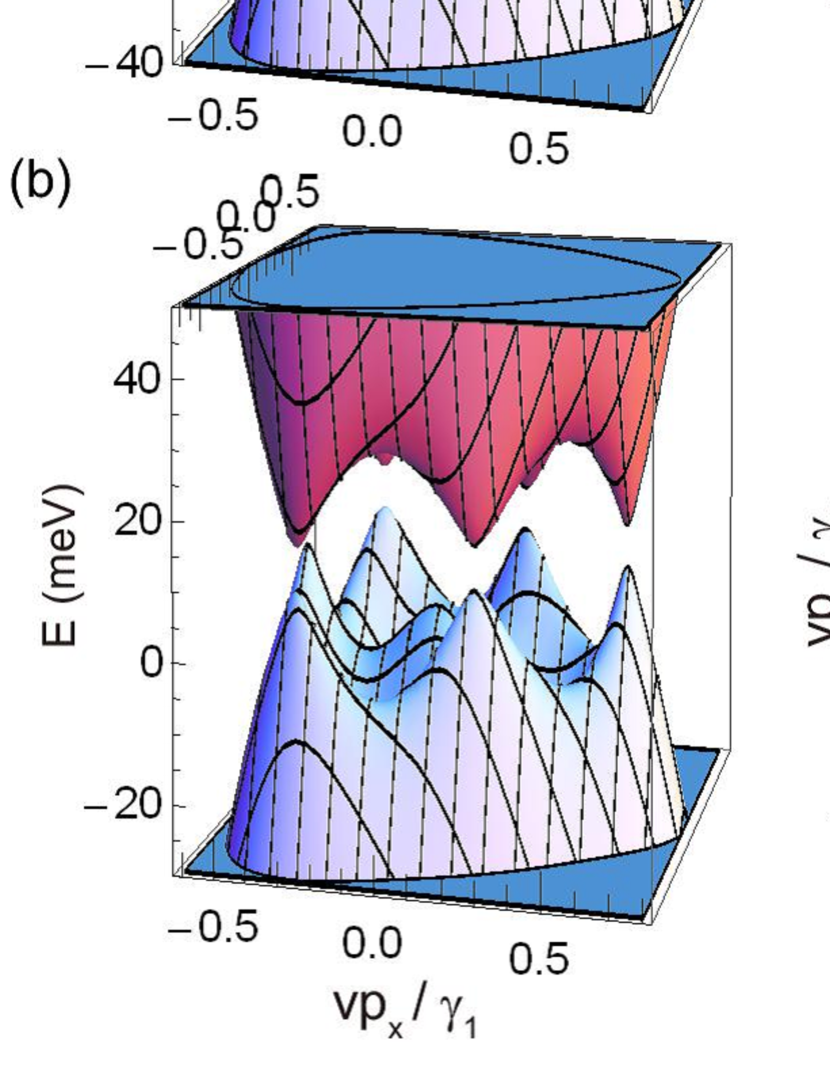
Figure 1: Band structures of ABA trilayer graphene in a perpendicular electric field depicted in 3D plot (left panel) and contour plot (right), for the band models (a) only with $v,\gamma_{1},v_{3}$ terms and (b) with full parameters. The interlayer potential asymmetry is set to be $\Delta=200$ meV.

In this paper, we closely study the band structures of ABA-stacked multilayer graphenes in the presence of uniform perpendicular electric field, and find that the interplay of the trigonal warping and the potential asymmetry generally gives rise to a number of additional Dirac cones nearly touching at zero energy, as depicted in Fig. 1(b) for trilayer graphene. For these gate-induced Dirac cones, the band velocity and the energy region (i.e., the distance between Dirac point to the Lifshitz transition point) are tunable with gate bias voltage. The energy region is typically a few tens of meV, which is by order of magnitude greater than in the original non-biased multilayer graphene. In a magnetic field, there arise triply-degenerate Landau levels originating from off-center gate-induced Dirac cones, with wide energy spacings due to the linear dispersion.

The gate-induced Dirac cones are generally gapped at Dirac point by symmetry-breaking terms. When the Fermi energy is in the gap, the system is in a topologically non-trivial valley Hall state, where electrons at $K_{+}$ and $K_{-}$ valleys carry opposite Hall conductivities Castro et al. (2008); Jung et al. (2011). A manifestation of the valley Hall state is the emergence of chiral edge modes at a zigzag interface which transports valley pseudo-spins in an analogous way to the spin Hall effect Murakami et al. (2003); Kane and Mele (2005). The valley Hall state and the helical edge modes were previously studied for gapped monolayer and bilayer graphenes, Castro et al. (2008); Tse et al. (2011); Qiao et al. (2011a, b, c, 2012) and also for ABC (rhombohedral) stacked trilayer graphene. Li et al. (2012) We study the edge states a semi-infinite zigzag ribbon of asymmetric ABA multilayer graphenes, and relate the number of the edge modes to the valley Hall conductivity which is a bulk property. In trilayer graphene, in particular, we find that non-zero valley Hall state is realized in a small external electric field, and moreover, a topological transition takes place at a certain higher electric field, which is accompanied by a change of the number of edge channels inside the bulk gap. In four-layer graphene, in contrast, the valley Hall conductivity is always zero and there are no edge modes filling the energy gap. We show that the nontrivial valley Hall state generally occurs in asymmetric odd layer graphenes, and this is deeply indebted to an approximate chiral symmetry peculiar to odd layer graphenes.

Paper is organized as follows. We briefly introduce the effective mass model for graphite in Sec. II, and argue the trilayer graphene in Sec. III in terms of the gate-induced Dirac cones, the chiral symmetry, the Landau level structure and and the edge states. In Sec. IV, we study the four-layer graphene as an example of even-layer cases without the chiral symmetry. In Sec. V, we argue the chiral symmetry in general odd-layer graphenes, generalizing the trilayer’s argument. The conclusion is given in Sec. VI.

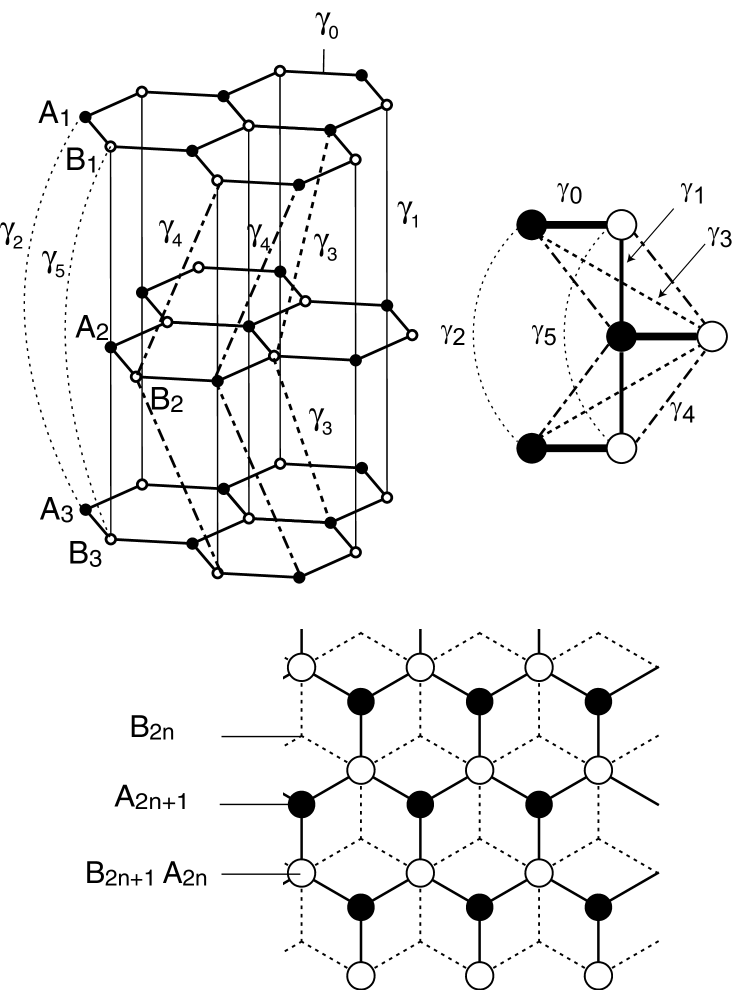
Figure 2: Lattice structure of ABA trilayer graphene with tight-binding hopping parameters. The bottom figure is a top-view, and the right is a schematic diagram of the lattice structure.

II Model

We describe the electronic properties of ABA-stacked multilayer graphene using Slonczewski-Weiss-McClure model Slonczewski and Weiss (1958); McClure (1960); Dresselhaus and Dresselhaus (2002) with hopping parameters described in Fig.2. The model includes intralayer coupling $\gamma_{0}$, nearest interlayer couplings $\gamma_{1}$, $\gamma_{3}$ and $\gamma_{4}$, next-nearest layer couplings $\gamma_{2}$ and $\gamma_{5}$, and on-site energy asymmetry $\Delta^{\prime}$, which are estimated in bulk graphite as Dresselhaus and Dresselhaus (2002): $\gamma_{0}=3.16$eV, $\gamma_{1}=0.39$eV, $\gamma_{3}=0.32$eV, $\gamma_{2}=-0.020$eV, $\gamma_{5}=0.038$eV, $\gamma_{4}=0.044$eV, $\Delta^{\prime}=0.050$eV. $\Delta^{\prime}$ is the energy difference between the sites which are involved in the coupling $\gamma_{1}$, and the sites which are not.

We consider ABA-stacked $N$-layer graphene, where $|A_{j}\rangle$ and $|B_{j}\rangle$ represent Bloch functions at the $K_{\xi}$ point, corresponding to the $A$ and $B$ sublattices of layer $j$, respectively. If the basis is arranged as $|A_{1}\rangle,|B_{1}\rangle$; $|A_{2}\rangle,|B_{2}\rangle$; $\cdots$; $|A_{N}\rangle,|B_{N}\rangle$, the Hamiltonian in the vicinity of the $K_{\xi}$ valley is written as Guinea et al. (2006); Partoens and Peeters (2006); Koshino and Ando (2007, 2008)

$${\cal H}=\begin{pmatrix}H_{0}&V&W&&\\ V^{\dagger}&H_{0}^{\prime}&V^{\dagger}&W^{\prime}&\\ W&V&H_{0}&V&W\\ &W^{\prime}&V^{\dagger}&H_{0}^{\prime}&V^{\dagger}&W^{\prime}&\\ &&\ddots&\ddots&\ddots\\ \end{pmatrix}+\begin{pmatrix}U_{1}\\ &U_{2}\\ &&U_{3}\\ &&&U_{4}\\ &&&&\ddots\end{pmatrix}$$ (1)

with

$$H_{0}=\begin{pmatrix}0&v\pi^{\dagger}\\ v\pi&\Delta^{\prime}\\ \end{pmatrix},H_{0}^{\prime}=\begin{pmatrix}\Delta^{\prime}&v\pi^{\dagger}\\ v\pi&0\\ \end{pmatrix},$$

$$V=\begin{pmatrix}-v_{4}\pi^{\dagger}&v_{3}\pi\\ \gamma_{1}&-v_{4}\pi^{\dagger}\\ \end{pmatrix},$$

$$W=\begin{pmatrix}\gamma_{2}/2&0\\ 0&\gamma_{5}/2\\ \end{pmatrix},W^{\prime}=\begin{pmatrix}\gamma_{5}/2&0\\ 0&\gamma_{2}/2\\ \end{pmatrix},$$

$$U_{j}=-\Delta\left(j-\frac{N+1}{2}\right)\begin{pmatrix}1&0\\ 0&1\\ \end{pmatrix}.$$

where $\pi=\xi\pi_{x}+i\pi_{y}$, $\mbox{\boldmath$\pi$}=\mbox{\boldmath$p$}+e\mbox{\boldmath$A$}$ with $A$ being the vector potential arising from the applied magnetic field, and $\xi=\pm 1$ are the valley indeces for $K_{\pm}$. The parameter $v=\sqrt{3}a\gamma_{0}/(2\hbar)$ is the band velocity for monolayer graphene, and $v_{3}=\sqrt{3}a\gamma_{3}/(2\hbar)$ a velocity related to the band parameter $\gamma_{3}$, where $a\approx 0.246$ nm is the distance between the nearest $A$ sites on the same layer. $U_{j}$ describes the electrostatic potential on $j$-th layer induced by the external electric field, where we assumed a uniform potential gradient in the perpendicular direction, This is valid in a few-layer graphene with typically $N<\sim 5$. For thicker multilayers with $N>\sim 10$, the potential drop occurs within a few layers near the external gate due to the screening by the charge carriers in graphene. Koshino and McCann (2009); Koshino (2010)

III Trilayer graphene

III.1 Chiral symmetry and gate-induced Dirac cones

The Hamiltonian of ABA-trilayer graphene is given by Eq. (1) with $N=3$, where the external potential is $(U_{1},U_{2},U_{3})=(\Delta,0,-\Delta)$. In the absence of $\Delta$, the Hamiltonian can be block diagonalized into monolayer-like band and bilayer-like band. Koshino and McCann (2009) In finite $\Delta$, these sub-blocks are hybridized, and it is then useful to arrange the basis as

$$\bigl{\{}(|A_{1}\rangle-|A_{3}\rangle)/\sqrt{2},\,\,|B_{2}\rangle,\,\,(|B_{1}\rangle+|B_{3}\rangle)/\sqrt{2},$$

$$\quad(|B_{1}\rangle-|B_{3}\rangle)/\sqrt{2},\,\,|A_{2}\rangle,\,\,(|A_{1}\rangle+|A_{3}\rangle)/\sqrt{2}\bigr{\}},$$ (2)

where the monolayer-like band correspond to 1st and 4th bases and bilayer-like band to 2nd, 3rd, 5th, and 6th. We categorize the first three bases in Eq. (2) as group $\circ$, and the last three as group $\bullet$. The Hamiltonian is written in this basis as

$${\cal H}=\begin{pmatrix}H_{\circ}&D_{-}\\ D_{+}&H_{\bullet}\end{pmatrix}$$ (3)

$$D_{+}=\left(\begin{array}[]{ccc}v\pi&0&\Delta\\ 0&v\pi^{\dagger}&\sqrt{2}\gamma_{1}\\ \Delta&\sqrt{2}v_{3}\pi&v\pi^{\dagger}\end{array}\right),\quad D_{-}=(D_{+})^{\dagger}$$ (7)

$$H_{\circ}=\left(\begin{array}[]{ccc}-\gamma_{2}/2&0&0\\ 0&0&-\sqrt{2}v_{4}\pi\\ 0&-\sqrt{2}v_{4}\pi^{\dagger}&\gamma_{5}/2+\Delta^{\prime}\end{array}\right)$$ (11)

$$H_{\bullet}=\left(\begin{array}[]{ccc}-\gamma_{5}/2+\Delta^{\prime}&0&0\\ 0&\Delta^{\prime}&-\sqrt{2}v_{4}\pi\\ 0&-\sqrt{2}v_{4}\pi^{\dagger}&\gamma_{2}/2\end{array}\right)$$ (15)

If we keep only relevant band parameters $\gamma_{0}$, $\gamma_{1}$, $\gamma_{3}$ and the potential $\Delta$, and neglect remaining parameters, the Hamiltonian Eq. (3) possesses the chiral symmetry (sublattice symmetry), in that the diagonal matrix blocks $H_{\circ}$ and $H_{\bullet}$ all vanish, leaving the off-diagonal blocks $D_{\pm}$ which connects the bases of $\circ$ to the bases of $\bullet$. The reason for this can be understood in terms of reflection symmetry as follows: In the group $\circ$($\bullet$), the bases associated with $A$ and $B$ sublattices have odd and even (even and odd) parity, respectively, with respect to the reflection in the middle layer. The Hamiltonian without $\Delta$, i.e., the first term in Eq. (1) has even parity in the reflection, and has matrix elements only between $A$ and $B$ sublattices when only $\gamma_{0}$, $\gamma_{1}$ and $\gamma_{3}$ are kept. After the unitary transformation, it does not give any matrix elements in $H_{\circ}$ or $H_{\bullet}$ because in each group ($\circ$ or $\bullet$), a base associated with $A$ and one associated with $B$ always have different parity from the definition. On the other hand, the potential term, i.e., the second term in Eq. (1) is odd in the reflection and matrix elements only connect the same sublattice. It gives no matrix elements in $H_{\circ}$ or $H_{\bullet}$ either, because in each group, bases associated with the same sublattice always have the same parity.

The energy spectrum of this simplified Hamiltonian contains a single center Dirac cone and six off-center Dirac cones at zero energy, as depicted in Fig.1(a). The robustness of gapless spectrum is protected by the chiral symmetry. The extra terms with $\gamma_{2},\gamma_{5},v_{4}$ and $\Delta^{\prime}$ in the diagonal blocks break the chiral symmetry and open small energy gaps at these Dirac cones as in Fig.1(b).

The positions of the Dirac points in the chiral Hamiltonian without $H_{\circ}$ and $H_{\bullet}$ can be found by solving ${\rm det}\,D_{+}=0$ with $\pi=\xi p_{x}+ip_{y}=pe^{i\theta}$. We obtain a Dirac point at $p=0$, and six off-center Dirac points at

$$p=p_{+};\quad\theta=0,\frac{2\pi}{3},\frac{4\pi}{3},$$

$$p=p_{-};\quad\theta=\frac{\pi}{3},\pi,\frac{5\pi}{3},$$

$$p_{\pm}=\frac{\pm\gamma_{1}v_{3}+\sqrt{\Delta^{2}v^{2}+\gamma_{1}^{2}v_{3}^{2}}}{v^{2}}.$$ (16)

At each Dirac point, the degenerate zero-energy bases $\psi_{\circ}$ and $\psi_{\bullet}$ are derived from the equation $D_{+}|\psi_{\circ}\rangle=0$ and $D_{-}|\psi_{\bullet}\rangle=0$, and the effective Dirac Hamiltonian is given by

$$H_{\rm eff}=\begin{pmatrix}0&\langle\psi_{\circ}|D_{-}|\psi_{\bullet}\rangle\\ \langle\psi_{\bullet}|D_{+}|\psi_{\circ}\rangle&0\end{pmatrix},$$ (17)

keeping the lowest order in the momentum shift from the Dirac point. By rotating $(x,y)$ coordinate and the spinor space by angle $\theta$ at the same time, this is transformed to

$$H_{\rm eff}=v_{x}\tilde{\pi}_{x}\sigma_{x}+v_{y}\tilde{\pi}_{y}\sigma_{y},$$ (18)

where $\sigma_{x}$ and $\sigma_{y}$ are Pauli matrices, and $(\tilde{\pi}_{x},\tilde{\pi}_{y})$ is the momentum measured from each Dirac point. We find for the Dirac point at $p=0$ (no need for rotation),

$$\psi_{\circ}=(0,1,0)$$

$$\psi_{\bullet}=(-\sqrt{2}\gamma_{1},\Delta,0)/\sqrt{\Delta^{2}+2\gamma_{1}^{2}},$$ (19)

and

$$v_{x}=\xi\frac{\Delta v}{\sqrt{\Delta^{2}+2\gamma_{1}^{2}}},\quad v_{y}=-\frac{\Delta v}{\sqrt{\Delta^{2}+2\gamma_{1}^{2}}}.$$ (20)

with the valley index $\xi=\pm$. For the off-center Dirac points at $p=p_{\pm}$,

$$\psi_{\circ}=(-\Delta e^{i\theta},\mp\sqrt{2}\gamma_{1},vp_{\pm}e^{2i\theta})/C_{1},$$

$$\psi_{\bullet}=(-\Delta,\mp\sqrt{2}v_{3}p_{\pm},vp_{\pm}e^{-i\theta})/C_{2},$$

$$C_{1}=\sqrt{\Delta^{2}+2\gamma_{1}^{2}+v^{2}p_{\pm}^{2}},C_{2}=\sqrt{\Delta^{2}+(2v_{3}^{2}+v^{2})p_{\pm}^{2}},$$

and the velocities after rotation of $(x,y)$ by $\theta$ become

$$v_{x}=2\xi v(\pm\Delta^{2}+\gamma_{1}v_{3}p_{\pm})/(C_{1}C_{2})$$

$$v_{y}=-6\gamma_{1}v_{3}vp_{\pm}/(C_{1}C_{2}),$$ (22)

where $v_{x}$ and $v_{y}$ correspond to the radial and azimuthal directions respectively, with respect to $p=0$. $v_{x}$ and $v_{y}$ of each Dirac points are plotted in Fig. 3(d). The velocities are mainly enhanced by applying $\Delta$, while $v_{y}$ for $p_{+}$ decreases only slowly. This indicates that the conductivity, which is roughly proportional to the square of the band velocity Shon and Ando (1998), is enhanced by $\Delta$, as is consistent with the previous transport measurement Craciun et al. (2009) and the theoretical estimation Koshino and McCann (2009).

The chirality for each Dirac cone can be defined by $\nu_{c}\equiv\textrm{sgn}(v_{x}v_{y})$, and this coincides with the Berry phase in units of $\pi$ around the Dirac point. We find $\nu_{c}=-\xi$ for $p=0$, and $\nu_{c}=\mp\xi$ for $p=p_{\pm}$, so that the summation of chirality over seven Dirac points in the valley $K_{\xi}$ is $-\xi$. Since the chirality is a topologically protected number as long as the chiral symmetry is present, non-zero total chirality indicates that the conduction band and the valence band inevitably touch at some points in any value of $\Delta$.

Now we consider all the band parameters in Eq. (3) to argue the energy gaps at the Dirac points. The effective Hamiltonian of each gate-induced Dirac cone is modified to

$$H_{\rm eff}=v_{x}\tilde{\pi}_{x}\sigma_{x}+v_{y}\tilde{\pi}_{y}\sigma_{y}+m\sigma_{z}+\epsilon_{0}I,$$ (23)

where the mass $m$ and the energy shift $\epsilon_{0}$ are given by

$$m=[\langle\psi_{\circ}|H_{\circ}|\psi_{\circ}\rangle-\langle\psi_{\bullet}|H_{\bullet}|\psi_{\bullet}\rangle]/2,$$ (24)

$$\epsilon_{0}=[\langle\psi_{\circ}|H_{\circ}|\psi_{\circ}\rangle+\langle\psi_{\bullet}|H_{\bullet}|\psi_{\bullet}\rangle]/2.$$ (25)

The width of the energy gap is $2m$. Note that the approximation using the gapped Dirac Hamiltonian above is valid when the mass gap is smaller than the energy region of the gate-induced Dirac cone below the Lifshitz transition point. In Fig.3(c), we show the evaluated mass $m$ for the seven Dirac points. We see that the mass for $p=p_{-}$ changes from negative to positive when $\Delta$ exceeds the critical value,

$$\Delta_{c}\approx 270\,{\rm meV},$$ (26)

at which the energy gap closes.

$$\begin{array}[]{c|ccc}p&0(\times 1)&p_{+}(\times 3)&p_{-}(\times 3)\\ \hline\cr{\rm sgn}(v_{x}v_{y})&-\xi&-\xi&+\xi\\ \hline\cr{\rm sgn}(m)&-1&+1&\begin{cases}-1~{}~{}(\Delta<\Delta_{c})\\ +1~{}~{}(\Delta>\Delta_{c})\end{cases}\\ \hline\cr{\rm sgn}(v_{x}v_{y}m)&+\xi&-\xi&\begin{cases}-\xi~{}~{}(\Delta<\Delta_{c})\\ +\xi~{}~{}(\Delta>\Delta_{c})\end{cases}\end{array}$$

Table 1: Sign of chirality, mass and in-gap Hall conductivity for gate-induced Dirac cones at $K_{\xi}$ valley.

When the Fermi energy lies in the gap in massive Dirac Hamiltonian Eq. (23), the Hall conductivity takes non-zero value $\sigma_{xy}=[e^{2}/(2h)]{\rm sgn}(v_{x}v_{y}m)$ even in zero magnetic field. Haldane (1988); Oshikawa (1994) Considering chirality and mass for each Dirac point in Table 1, the total Hall conductivity summed over the Dirac points at single valley $K_{\xi}$ becomes

$$\sigma_{xy}^{K_{\xi}}=\frac{e^{2}}{h}\times\left\{\begin{array}[]{cc}\displaystyle-\frac{5}{2}\xi&(\Delta<\Delta_{c}),\vspace{2mm}\\ \displaystyle+\frac{1}{2}\xi&(\Delta>\Delta_{c}).\end{array}\right.$$ (29)

We have a topological change at gap closing point, $\Delta=\Delta_{c}$. The Hall conductivity have opposite signs between two valleys $K_{\pm}$ due to the time-reversal symmetry, so that the net Hall conductivity is always zero. Nevertheless, the single-valley Hall conductivity is directly related to the number of chiral edge modes appearing in zigzag edge, as we will see in Sec. III.3.

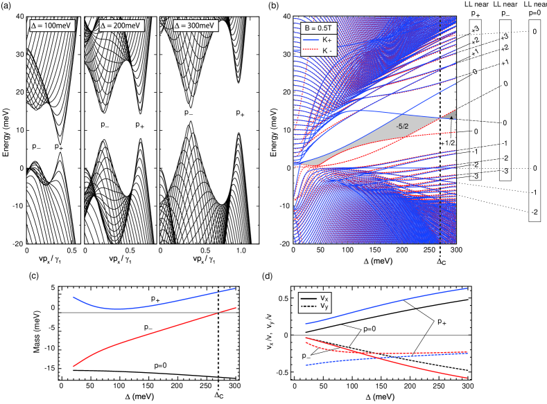
Figure 3: (a) Band structure of gated ABA trilayer with various potential asymmetry $\Delta$. (b)Gate bias dependence of Landau level energy in $B=0.5$T. Landau levels in $K_{+}$ and $K_{-}$ valleys are plotted as solid (blue) and dashed (red) lines, respectively. Shaded area represents the charge neutral region, where the number indicates the single valley Hall conductivity $\sigma_{xy}^{K\xi}$ in units of $\xi e^{2}/h$ (c) Effective mass $m$ and (d) band velocities $v_{x},v_{y}$ for the effective Dirac cones at $p=0,p_{+},p_{-}$, plotted against $\Delta$.

III.2 Landau level structure

The Landau levels in the presence of a uniform magnetic field $\mbox{\boldmath$B$}=(0,0,B)$ can be calculated by the Hamiltonian with $\pi=(\sqrt{2}\hbar/\ell)a^{\dagger}$ and $(\sqrt{2}\hbar/\ell)a$ for $K_{+}$ and $K_{-}$, respectively. Here $a^{\dagger}$ and $a$ are raising and lowering operators, respectively, which operate on the Landau-level wave function $\phi_{n}$ as $a\phi_{n}=\sqrt{n}\phi_{n-1},a^{\dagger}\phi_{n}=\sqrt{n+1}\phi_{n+1}$, and $\ell=\sqrt{\hbar/(eB)}$ is the magnetic length. The Landau level spectrum at $B=0.5$T is plotted as a function of potential asymmetry $\Delta$ in Fig.3(b). Landau levels in $K_{+}$ and $K_{-}$ valleys are plotted as solid (blue) and dashed (red) lines, respectively. There we can see two distinct regions, a region around zero energy where the Landau level spacing are wide due to Dirac Landau levels, and a region above the Lifshitz transition where the Landau levels are densely spaced due to large density of states. In increasing $\Delta$, the gate-induced Dirac pockets accommodate more and more Landau levels as the energy region within the Dirac pockets expands.

The low-energy Landau levels inside the gate-induced Dirac pockets can be approximately described by the massive Dirac Hamiltonian, Eq. (23). There the Landau level spectrum is explicitly written as

$$\begin{cases}E_{0}=\epsilon_{0}-{\rm sgn}(v_{x}v_{y})\,m,\\ E_{\pm n}=\epsilon_{0}\pm\sqrt{\Delta_{B}^{2}n+m^{2}},~{}~{}~{}(n>0),\end{cases}$$ (30)

where

$$\Delta_{B}=\sqrt{2|v_{x}v_{y}|\hbar eB}.$$ (31)

We note that the Landau level of $n=0$ is sensitive to the chirality and the sign of the mass: it appears at the top of the valence band and the bottom of the conduction band when ${\rm sgn}(v_{x}v_{y}m)>0$ and $<0$, respectively. The two cases correspond to the mid-gap values of the Hall conductivity, $\sigma_{xy}=e^{2}/(2h)$ and $-e^{2}/(2h)$, respectively. Also, since the chirality ${\rm sgn}(v_{x}v_{y})$ is opposite between $K_{+}$ and $K_{-}$ valleys, the $n=0$ Landau level split in valleys, while all others are valley degenerate. Besides, we have additional triple-fold degeneracies for each of $p_{+}$ and $p_{-}$.

In Fig.3(b), we actually see that the levels $n=0$ level is non-degenerate in valleys, appearing at either of the band edges of each massive Dirac band. At $\Delta=\Delta_{c}$, we observe that one pair of $n=0$ levels from $K_{\pm}$ valleys crosses each other at the charge neutral point, in accordance with the topological change of $\sigma_{xy}^{K_{\xi}}$ from $(-5/2)\xi e^{2}/h$ to $(+1/2)\xi e^{2}/h$. The levels $n>0$ are almost valley-degenerate while tiny splitting is due to the deviation from the massive Dirac Hamiltonian Eq. (23).

When we drop the band parameters other than $\gamma_{0},\gamma_{1}$ and $\gamma_{3}$, the Hamiltonian becomes chiral symmetric and the zero-th Landau level $E_{0}$ of each Dirac cone comes exactly to zero energy as a chiral zero mode, of which wavefunction has amplitude only on $\circ$ and $\bullet$ for $\nu_{c}=\mp\xi$, respectively. The index theorem then states that the difference between the number of the zero-modes belonging to $\circ$ $(n_{+})$ and those to $\bullet$ $(n_{-})$, is defined as chiral index, which coincides with the gauge flux penetrating the system. The chiral index in the present case is shown to be $n_{+}-n_{-}=\xi\Phi$ where $\Phi=eBS/h$ is the magnetic flux penetrating the system area $S$. This is, in units of $\Phi$, coherent with a summation of $-\nu_{c}$ in each single valley. As in the conventional Dirac Hamiltonian, Jackiw and Rebbi (1977); Fujikawa (1979); Fujikawa and Suzuki (2004) the chiral index can be related to the geometric curvature of the gauge field, and the above relation between the chiral index and total magnetic flux stands in non-uniform magnetic field as well. The detailed argument is presented in Appendix. A.

III.3 Edge modes

Non-trivial Hall conductivity in single valley indicates an existence of chiral edge modes localized at the interface, as long as the valley mixing is not present. There the number of emergent edge modes are directly related to the Hall conductivity, so that chiral edge modes as many as the number of $\sigma_{xy}^{K_{\pm}}$ should counterflow in opposite directions between $K_{+}$ and $K_{-}$, as is analogous to the spin Hall insulator.Murakami et al. (2003) Here we numerically examined the edge modes in the asymmetric ABA trilayer graphene with zigzag interfaces, in which the valley mixing is absent. We consider a semi-infinite system with a zigzag boundary along $x$ direction as shown in Fig. 4(a), where $p_{x}$ is a good quantum number. The energy of edge modes in the bulk gap can be obtained by searching for the evanescent modes satisfying a boundary condition at the interface. The method is detailed in Appendix B.

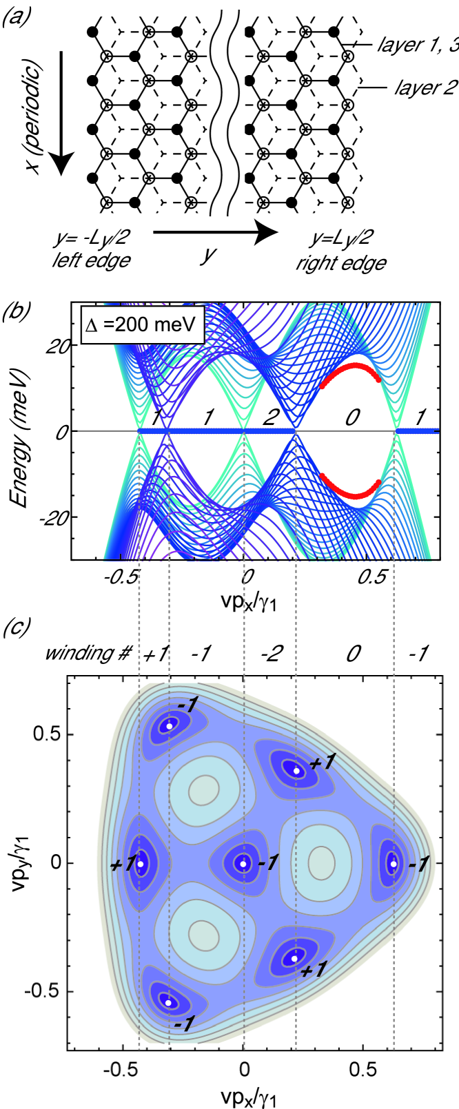
Figure 4: (a) Atomic structure of a zigzag ribbon of ABA trilayer graphene. (b) Band structure around $K_{+}$ valley of a zigzag ribbon of ABA trilayer graphene only including $\gamma_{0},\gamma_{1}$ and $\gamma_{3}$, with the asymmetric potential $\Delta=200$ meV. Bulk, left-edge and right-edge states are plotted with solid lines, red dots and blue dots, respectively. Numbers indicate the degeneracies of the edge state bands for a single side (the same for the left and the right edges). (c) Contour plot of the bulk band structure with white dots and labels denoting the position and the chirality of gate-induced Dirac points, respectively. One-dimensional winding number $\gamma(k_{x})$ is indicated between dotted lines penetrating the Dirac points.

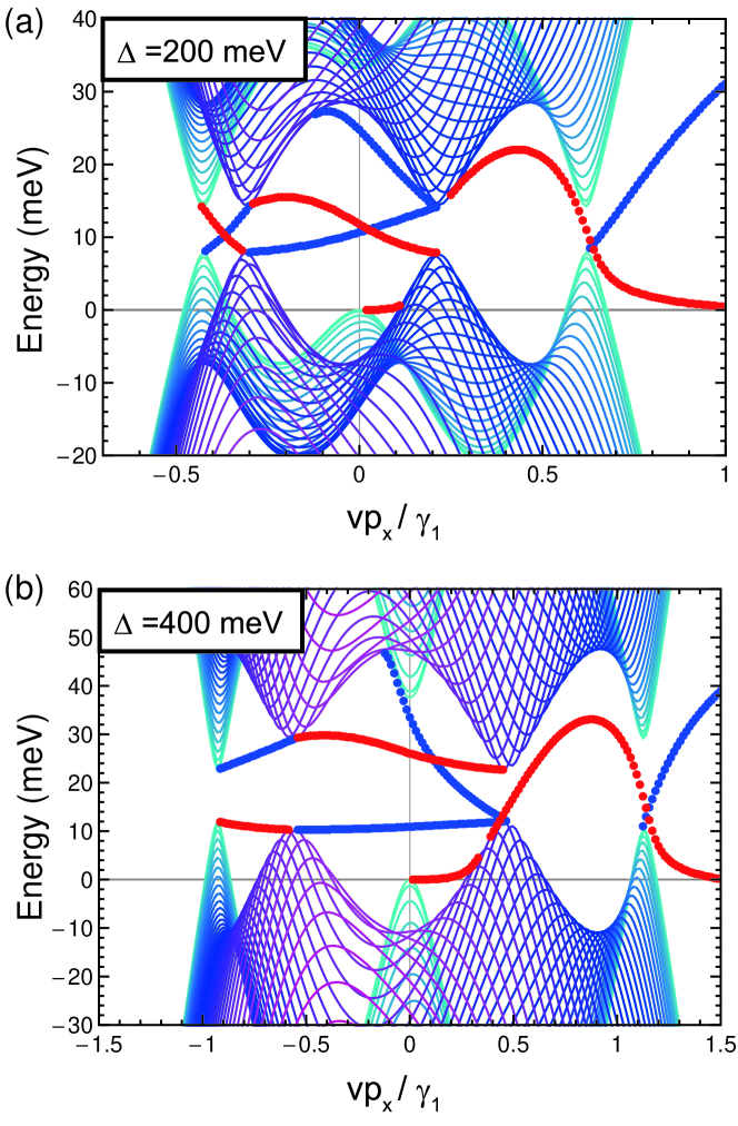
Figure 5: Band structure around $K_{+}$ valley of zigzag ribbon of ABA trilayer graphene with the parameters fully included, in the asymmetric potential (a) $\Delta=200$ meV and (b) $\Delta=400$ meV. Bulk, left-edge and right-edge states are plotted with solid lines, red dots and blue dots, respectively.

First we consider the chiral symmetric case neglecting $\gamma_{2},\gamma_{5},v_{4},\Delta^{\prime}$. Fig.4 illustrates the energy spectrum near $K_{+}$ point at $\Delta=200$ meV, where we see that zero-energy edge modes appear between some of gate-induced Dirac points. The number of zero energy edge modes are closely related to the chirality of each Dirac cone. Ryu and Hatsugai (2002); Schnyder and Ryu (2011); Heikkilä and Volovik (2011); Burkov et al. (2011) When we regard a two-dimensional periodic system on $xy$-plane as a one-dimensional system with fixed $p_{x}$ as a parameter, we can define a winding number $\gamma(p_{x})$ by integrating the Berry phase change all the way along $p_{y}$ on the Brillouin zone at the fixed $p_{x}$. When we set the boundary perpendicular to $y$ axis (i.e., $p_{x}$ is still a good quantum number), the number of zero-energy edge modes appearing at the boundary coincides with $\gamma(p_{x})$ except a constant.Ryu and Hatsugai (2002) In the present system, this bulk-edge relationship can be clearly seen in Fig.4.

Other hopping terms breaking the chiral symmetry give rise to mass to the Dirac points, and relative signs between these masses determines the connection of the chiral edge modes between different Dirac points. In Fig.5(a), we plot the band structure near $K_{+}$ including full band parameters at $\Delta=200$ meV. We see that the left and right edge modes stick to either of the top or bottom of gapped Dirac cone depending on the sign of the mass. At the charge neutral point, we have three set of chiral edge channels crossing the Fermi energy, which all circulate in clockwise direction when viewed from $+z$ direction. We also observe two edge states extending out of the plot and leading to the other valley $K_{-}$. In $K_{-}$, we have the exactly same spectrum with $p_{x}$ inverted to $-p_{x}$.

The correspondence to the single-valley Hall conductivity can be understood in a similar argument to that for integer quantum Hall effect.Laughlin (1981) Let us consider a cylindrical system which is closed in $x$ with circumference $L_{x}$ while finite in the axial direction $y$ with $-L_{y}/2<y<L_{y}/2$ bound by the zigzag edges. When we adiabatically turn on a magnetic flux quantum $h/e$ penetrating into the cylinder (inducing an electric field along $-x$ direction), every state at $p_{x}$ is shifted to $p_{x}+2\pi\hbar/L_{x}$. The single-valley Hall conductivity of $K_{+}$ then coincides with the total move of $K_{+}$ electrons in $-y$ direction through this adiabatic process. At the Fermi energy, an electron moves from the left edge to the right for each of three pairs of counter-propagating channels, contributing to $\sigma_{xy}^{K_{+}}=-3e^{2}/h$. A charge transfer also occurs below the Fermi energy, where a bulk state $(\langle y\rangle=0)$ is pumped to an edge state $(\langle y\rangle=-L_{y}/2)$ in the left-edge channel going out of the valley. This yields a contribution to $\sigma_{xy}^{K_{+}}=(+1/2)e^{2}/h$, which adds up to $\sigma_{xy}^{K_{+}}=(-5/2)e^{2}/h$ all together.

Fig.5(b) plots the band structure at larger bias, $\Delta=400$ meV after the topological transition at $\Delta_{c}$. We find that the connection of the edge modes changes at $p=p_{-}$, leaving only one clockwise and one anti-clockwise chiral edge modes crossing at the Fermi energy. The Hall conductivity from those two exactly cancel out, while we have the same contribution from the edge channel below the Fermi energy, giving the total Hall conductivity $\sigma_{xy}^{K_{+}}=(+1/2)e^{2}/h$. This again coincides with bulk valley Hall conductivity estimated from the mass and chirality. Conversely, the single valley Hall conductivity gives the number of the counter edge modes crossing at the Fermi energy, when we appropriately exclude the half integer contribution from the edge modes connecting $K_{\pm}$.

IV Four-layer graphene

Unlike trilayer, a four-layer graphene with interlayer asymmetry does not possess the chiral symmetry even in the approximate model, and the band gap always open at the zero energy. The effective low-energy Hamiltonian can be obtained by excluding the high-energy bonding states at $|\varepsilon|\sim O(\gamma_{1})$ as $H_{\rm eff}=H_{11}-H_{12}H_{22}^{-1}H_{21}$,McCann and Fal’ko (2006) where $H_{11}$ and $H_{22}$ represent diagonal blocks of the original Hamiltonian for low-energy bases spanned by $(A1,B2,A3,B4)$, and for high-energy bases by $(B1,A2,B3,A4)$, respectively, and $H_{12}$ and $H_{21}$ are off-diagonal blocks connecting them. This is explictly written in basis $(A1,B2,A3,B4)$ as

$$H_{\rm eff} = \frac{v^{2}}{\gamma_{1}}\begin{pmatrix}0&-(\pi^{\dagger})^{2}&0&(\pi^{\dagger})^{2}\\ -\pi^{2}&0&0&0\\ 0&0&0&-(\pi^{\dagger})^{2}\\ \pi^{2}&0&-\pi^{2}&0\\ \end{pmatrix}$$ (32)

$$+ v_{3}\begin{pmatrix}0&\pi&&\\ \pi^{\dagger}&0&\pi^{\dagger}&\\ &\pi&0&\pi\\ &&\pi^{\dagger}&0\\ \end{pmatrix}+\Delta\begin{pmatrix}\frac{3}{2}\\ &\frac{1}{2}\\ &&-\frac{1}{2}\\ &&&-\frac{3}{2}\end{pmatrix},$$

where we neglected the band parameters other than $\gamma_{0},\gamma_{1}$ and $\gamma_{3}$. The approximation is valid only when $vp,\Delta\ll\gamma_{1}$.

If we even neglect $v_{3}$ term, the low-energy energy band is rotationally symmetric around $K\pm$ points and its dispersion relation is given by

$$\epsilon(p)=\pm\frac{1}{2}\sqrt{6\tilde{\epsilon}^{2}+5\Delta^{2}-2\sqrt{5\tilde{\epsilon}^{4}+20\tilde{\epsilon}^{2}\Delta^{2}+4\Delta^{4}}}$$ (33)

with $\tilde{\epsilon}=v^{2}p^{2}/\gamma_{1}$. The band gap appears between $\varepsilon=\pm(\Delta/2)(-7+16/\sqrt{5})^{1/2}$, corresponding to an off-center momentum $p_{0}=(-2+6/\sqrt{5})^{1/4}\sqrt{\gamma_{1}\Delta}/v$.

When we resume $v_{3}$ term and other parameters, six off-center pockets emerge at momentum $p_{+}$ and $p_{-}$ near $p_{0}$, each of which are arranged in 120 degrees symmetry as illustrated in Fig.6, and Fig.7(a). The pre-existent gap never closes during this process. The pockets at $p=p_{+}$ are much deeper than those at $p=p_{-}$, and the energy depth is about 15 meV at $\Delta=100$ meV. Fig.7(b) describes an evolution of Landau level energies with increasing $\Delta$, where we observe the triply-degenerate Landau levels of $p_{+}$ pockets with wide energy spacing, similarly to trilayer graphene.

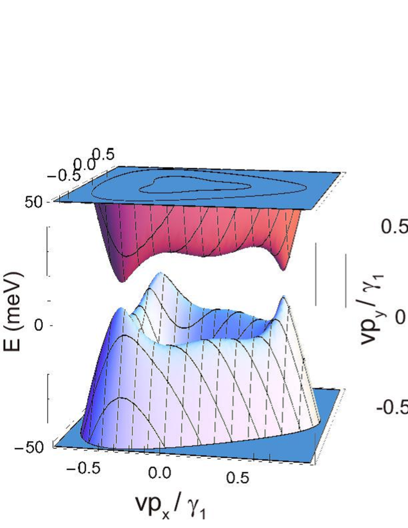
Figure 6: Band structures of ABA-stacked fourlayer graphene with the interlayer asymmetric potential $\Delta=100$ meV, depicted in 3D plot (left panel) and contour plot (right).

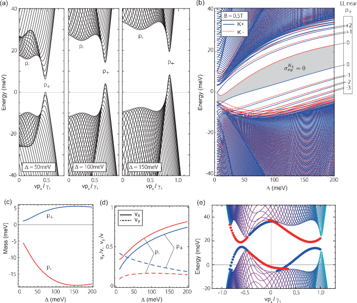
Figure 7: Plots similar to Fig. 3 for ABA fourlayer graphene. (a) Band structure with various potential asymmetry $\Delta$. (b) Gate bias dependence of Landau level energy in $B=0.5$T. Shaded area represents the charge neutral region. (c) Effective mass $m$ and (d) band velocities $v_{x},v_{y}$ for the effective Dirac cones at $p_{+},p_{-}$, plotted against $\Delta$. (e) Band structure similar to Fig. 5 for zigzag ribbon of ABA fourlayer with $\Delta=200$meV.

We can expand the Hamiltonian with respect to the center of each Dirac pocket, and obtain the effective $2\times 2$ Hamiltonian in the massive Dirac form of Eq. (23). The masses and the velocities are shown in Fig.7(c) and (d), respectively, where we set the basis so that the chirality becomes $+1$ (i.e., $v_{x}v_{y}$ positive). The masses at $p_{+}$ and $p_{-}$ are opposite in sign, so that the contributions to the Hall conductivity of Dirac cones cancel out in summation over a single valley. Therefore, the single valley system is a trivial insulator with zero Hall conductivity in contrast to trilayer graphene. Accordingly, we observe no Landau level crossing at charge neutral point in Fig.7(b), and if we look at the edge states in Fig.7(e), there are no edge channel crossing in the bulk gap, nor the counter-propagating flows of valley pseudo-spin.

V General odd-layer graphenes

The approximate chiral symmetry in the presence of the external electric field argued in trilayer actually holds in any odd-layer Bernal multilayer graphenes. As we see in the following, if we only consider $\gamma_{0},\gamma_{1},\gamma_{3},\Delta$ terms , the Hamiltonian of odd layered graphene is chiral symmetric with a nonzero chiral index in the presence of magnetic field, which means that the band is gapless in limit of zero magnetic field.

The Hamiltonian for Bernal stacked $N$-layer graphene is decomposed into block diagonal form with effective monolayer and bilayer blocks with a unitary transformation Koshino and Ando (2007, 2008, 2009); Koshino and McCann (2011). Let us define

$$f_{m}(j)=c_{m}\sqrt{\frac{2}{N+1}}[1-(-1)^{j}]\sin\kappa_{m}j,$$

$$g_{m}(j)=c_{m}\sqrt{\frac{2}{N+1}}[1+(-1)^{j}]\sin\kappa_{m}j,$$ (34)

where

$$\kappa_{m}=\frac{\pi}{2}-\frac{m\pi}{2(N+1)},$$

$$c_{m}=\begin{cases}1/2&(m=0),\\ 1/\sqrt{2}&(m\neq 0),\\ \end{cases}$$ (35)

$j=1,2,...,N$ is the layer index, $m$ is the block index given as

$$m=\begin{cases}1,3,5,...,N-1;&N=\mbox{even},\\ 0,2,4,...,N;&N=\mbox{odd}.\\ \end{cases}$$

Then we take a basis

$$|\phi_{m}^{(X,{\rm odd})}\rangle=\sum_{j=1}^{N}f_{m}(j)|X_{j}\rangle,$$

$$|\phi_{m}^{(X,{\rm even})}\rangle=\sum_{j=1}^{N}g_{m}(j)|X_{j}\rangle,$$ (36)

where $X=A$ or $B$. A superscript $(X,{\rm odd/even})$ indicates that the wavefunction is nonzero only on the sublattice $X$ on the layer $j=$ odd/even.

With the basis set above, the Hamiltonian with $\Delta=0$ is block diagonalized with $m$. A block labeled by $m$ spanned by $\{|\phi_{m}^{(A,{\rm odd})}\rangle,|\phi_{m}^{(B,{\rm odd})}\rangle,|\phi_{m}^{(A,{\rm even})}\rangle,|\phi_{m}^{(B,{\rm even})}\rangle\}$ is dictated as $H(\lambda_{m})$ with $\lambda_{m}=2\cos\kappa_{m}$ and

$$H(\lambda)=\begin{pmatrix}0&v\pi^{\dagger}&0&\lambda v_{3}\pi\\ v\pi&0&\lambda\gamma_{1}&0\\ 0&\lambda\gamma_{1}&0&v\pi^{\dagger}\\ \lambda v_{3}\pi^{\dagger}&0&v\pi&0\\ \end{pmatrix},$$ (37)

where we only left the terms with $\gamma_{0},\gamma_{1},\gamma_{3}$, For the case of $m=0$, only two bases $|\phi_{m}^{(A,{\rm odd})}\rangle,|\phi_{m}^{(B,{\rm odd})}\rangle$ survive due to $g_{0}(j)=0$, and the corresponding block Hamiltonian is the first 2 by 2 component of Eq.(37).

Now let us consider an odd-layer graphene with the interlayer potential asymmetry $U(\Delta)$, i.e., the second term of Hamiltonian, Eq. (1). When $N={\rm odd}$, we can easily show that the basis function belonging to the block $m$ is either symmetric or antisymmetric with respect to reflection in the central layer $j=(N+1)/2$, and the parity is given by $(-1)^{(N-m-1)/2}$. Koshino and McCann (2011) If we write down $U(\Delta)$ in this basis, the matrix element $\langle\phi_{m^{\prime}}^{(X^{\prime},p^{\prime})}|U|\phi_{m}^{(X,p)}\rangle$ ($p,p^{\prime}=$ even or odd) becomes non-zero only when $m^{\prime}=m+4l+2(l:{\rm integer})$, $X=X^{\prime}$, and $p=p^{\prime}$, because $U$ is an odd function in the reflection, and also diagonal in the original site representation.

Therefore, if we separate the basis functions into two groups $\circ,\bullet$ as:

$$(|\phi_{m}^{(A,{\rm odd})}\rangle,|\phi_{m}^{(B,{\rm odd})}\rangle,|\phi_{m}^{(A,{\rm even})}\rangle,|\phi_{m}^{(B,{\rm even})}\rangle)$$

$$\qquad\qquad\in\begin{cases}(\circ,\bullet,\circ,\bullet)\quad(m=4l)\\ (\bullet,\circ,\bullet,\circ)\quad(m=4l+2),\end{cases}$$ (38)

then the Hamiltonian including only $\gamma_{0},\gamma_{1},\gamma_{3},\Delta$ has matrix elements only between $\circ$ and $\bullet$, and thus is chiral symmetric. Note that the chiral symmetry is not respected for even-layer graphenes since the basis function labeled by $m$ cannot be categorized to either even or odd parity, and the interlayer potential term gives rise to matrix elements connecting blocks $m$ and $m+4l$.

In the presence of magnetic field, the chiral index, i.e., the difference between the number of the zero-modes belonging to $\circ$ $(n_{+})$ and those to $\bullet$ $(n_{-})$, can be easily obtained by considering the Landau level spectrum with $\gamma_{1}$, $v_{3}$ and $\Delta$ all switched off, since the chiral index never changes in such a continuous transformation. The bilayer-like Hamiltonian block, Eq. (37), is then consists of two monolayer-type $2\times 2$ diagonal blocks, giving two zero-energy Landau levels localized at the second and fourth (first and third) elements in the valley $\xi=+(-)$. Considering the base grouping in Eq. (38), the difference in zero energy states in block $m$ is found to be $n_{+}-n_{-}=\mp 2\xi\Phi$ for $m=4l$ and $m=4l+2$, respectively, where $\Phi=eBS/h$ is the magnetic flux penetrating the system. The monolayer-type block $m=0$ lacks the third and fourth elements, giving $n_{+}-n_{-}=-\xi\Phi$. As a result, the total chiral index in odd-layer graphene for valley $K_{\xi}$ is finally given by

$$n_{+}-n_{-} = (-1+2-2+2\cdots)\xi\Phi$$ (39)

$$= \begin{cases}-\xi\Phi;&N=4l+1\\ +\xi\Phi;&N=4l+3.\\ \end{cases}$$

This states that at least one Landau level remains at zero energy, and thus in zero magnetic field, the conduction and valence band touch at one $k$-point at least. The sum of Berry phases in a single valley coincides with $-\pi$ times the chiral index in units of $\Phi$, that is $\pm\xi\pi$ for $N=4l+1$ and $4l+3$, respectively. When the Dirac cones are gapped by including the additional band parameters, the Hall conductivity per single valley must be non-zero, because the number of Dirac cones per valley must be odd to achieve total Berry phase $\pm\pi$.

The result might seem to contradict with the well-known fact that the Berry phase is $N\pi$ in $N$-layer graphene at $\Delta=0$. As argued, the Hamiltonian with $\Delta=0$ is block diagonalized into independent monolayer-like and bilayer-like subsystems. In each block, there is an ambiguity in the choice of bases for $\circ$ or $\bullet$, and the Berry phase of the block actually changes its sign when $\circ$ and $\bullet$ are interchanged. If we simply assign all $A$ and $B$ sublattices to $\circ$ and $\bullet$, respectively, we obtain $n_{+}-n_{-}=(-1-2-2-2\cdots)\xi\Phi=-\xi N\Phi$ instead of Eq. (39). In the presence of nonzero $\Delta$, on the other hand, the subsystems are mixed with each other and then the grouping of Eq. (38) is the only possible way to make the Hamiltonian chiral symmetric.

VI Conclusion

In Bernal multilayer graphene more than three layers, an interplay of the gate electric field and the trigonal warping effect gives rise to emergent Dirac cones in the low energy bands, whose band velocity and Lifshitz transition energy are tunable by the gate voltage. In trilayer graphene, in particular, the low-energy effective theory shows that the valley Hall state is realized at the charge neutral point, where single valley Hall conductivity is quantized at a non-zero half integer. We have investigated the edge states at the zigzag interface, and demonstrated that the number of edge modes is closely related to the bulk single valley Hall conductivity. In four-layer graphene, gate-induced Dirac cones also appear, though the system is a trivial insulator with zero valley Hall conductivity. The non-trivial valley Hall state is generally found in odd-layer graphenes, where the approximate chiral symmetry is responsible for the emergence of non-zero valley Hall conductivity.

The gate-induced Dirac cones should be experimentally accessible directly by observing Landau levels with wide energy spacing. Sadowski et al. (2006); Jiang et al. (2007); Morimoto et al. (2012) Also, the single valley Hall conductivity argued here is expected to be observable in the transport through the edge modes at a zigzag interface, while a valley mixing caused by a concentration of atomic-scale scatterers or a presence of armchair edge would wash out the effect. There the conductance is related to the number of edge channels, and the topological transition at $\Delta_{c}$ should be observed as a change in the conductance. Since the helical edge modes appearing in the gated multilayer graphene carry valley pseudospins, modulation of edge modes through the gate voltage could be a way to electrically control the valley polarized transport.

Appendix A Index theorem for odd-layer graphenes

Here we show that the chiral index of general odd-layer graphenes can be written in terms of the total gauge flux penetrating the system, in a similar way to the argument for usual Dirac Hamiltonian. Jackiw and Rebbi (1977); Fujikawa (1979); Fujikawa and Suzuki (2004) The chiral symmetric Hamiltonian of odd-layer graphene with interlayer asymmetric potential is written as

$$H=\begin{pmatrix}0&D_{-}\\ D_{+}&0\end{pmatrix},$$ (40)

where $D_{+}=(D_{-})^{\dagger}$ is a $N\times N$ matrix. The chiral symmetry is then expressed by $\Gamma H+H\Gamma=0$ with the chiral operator $\Gamma$,

$$\Gamma=\begin{pmatrix}\mbox{1}\mbox{l}_{N}&0\\ 0&-\mbox{1}\mbox{l}_{N}\\ \end{pmatrix},$$

where $\mbox{1}\mbox{l}_{N}$ is $N\times N$ unit matrix. We can take zero modes of $H$ as an eigenvector $\psi_{\pm}$ of $\Gamma$ with eigenvalue $\pm 1$, respectively. If we write the number of chiral zero modes $\psi_{\pm}$ as $n_{\pm}$, the chiral index $\nu$ is defined as

$$\nu=n_{+}-n_{-}=\mbox{Tr}\Gamma f(H^{2}/M^{2}),$$

where $f$ is a regularization function, which is smooth and monotonically decreasing function with $f(0)=1$ and $f(\infty)=0$, and $M$ is an ultraviolet cutoff. The action of $f$ to the matrix is defined through its action onto the eigenvalues, as seen if we take $f(z)=e^{-z}$.

If we take plane waves $\exp(i\mbox{\boldmath$k$}\cdot\mbox{\boldmath$x$})$ as a basis for the spatial direction, we have

$$\nu = \mbox{Tr}\Gamma f(H^{2}/M^{2})$$

$$= \mbox{Tr}[f(D_{-}D_{+}/M^{2})-f(D_{+}D_{-}/M^{2})]$$

$$= \int d^{2}x\int\frac{d^{2}k}{(2\pi)^{2}}\mbox{tr}\,e^{-ikx}[f(D_{-}D_{+}/M^{2})$$

$$\qquad\qquad\qquad-f(D_{+}D_{-}/M^{2})]e^{ikx}$$

where Tr means a trace over all the states while tr is a trace over the layer and site indeces or, equivalently, $m$, $X$ and even/odd indices in Eq.(36).

The operator $\pi$ acts on a plane wave to give $e^{-ikx}\mbox{\boldmath$\pi$}e^{ikx}=\hbar\mbox{\boldmath$k$}+\mbox{\boldmath$\pi$}$. Since $D_{\pm}$ contains at most first order derivative terms, we can write

$$e^{-ikx}D_{+}e^{ikx}=D_{0}|\mbox{\boldmath$k$}|+D_{+}$$

$$e^{-ikx}D_{-}e^{ikx}=D_{0}^{\dagger}|\mbox{\boldmath$k$}|+D_{-},$$

where $D_{0}$ is a c-number matrix and of zero-th order in $|\mbox{\boldmath$k$}|$, but may depend on a polar angle of $k$. Since $D_{0}$ is a square matrix, it can be written in a singular value decomposition

$$D_{0}=U\Sigma V^{\dagger}$$

with unitary matrices $U,V$ and a diagonal matrix $\Sigma=\mbox{diag}(\sqrt{\lambda_{i}})$ $(\lambda_{i}\geq 0)$.

The action of $D_{-}D_{+}$ on a plane wave is then described as

$$e^{-ikx}D_{\mp}D_{\pm}e^{ikx}=G_{\pm}k^{2}+F_{\pm},$$

where

$$G_{+}=D_{0}^{\dagger}D_{0}=V\Sigma^{2}V^{\dagger}$$

$$G_{-}=D_{0}D_{0}^{\dagger}=U\Sigma^{2}U^{\dagger},$$

are c-number matrices of zero-th order in $|\mbox{\boldmath$k$}|$. $F_{\pm}$ are matrices including the operator $\pi$, and up to first order of $|\mbox{\boldmath$k$}|$.

Having in mind that the ultraviolet behavior ($\hbar vk\sim M$) is important for the contribution of $D_{-}D_{+}$ term to the chiral index, we obtain

$$\mbox{tr}\{e^{-ikx}f(D_{-}D_{+}/M^{2})e^{ikx}\}$$

$$= \mbox{tr}\{Vf(k^{2}\Sigma^{2}/M^{2}+V^{\dagger}F_{+}V/M^{2})V^{\dagger}\}$$

$$= \mbox{tr}\{f(k^{2}\Sigma^{2}/M^{2})+f^{\prime}(k^{2}\Sigma^{2}/M^{2})(V^{\dagger}F_{+}V)/M^{2}\}$$

$$\hskip 180.00027pt+O(M^{-4})$$

$$= \sum_{i}\{f(k^{2}\lambda_{i}/M^{2})+f^{\prime}(k^{2}\lambda_{i}/M^{2})(V^{\dagger}F_{+}V)_{ii}/M^{2})\}$$

$$\hskip 180.00027pt+O(M^{-4})$$

With a similar form for $D_{+}D_{-}$ term, the chiral index with $M\to\infty$ reduces to

$$\nu = \int d^{2}x\int\frac{d^{2}k}{(2\pi)^{2}}\sum_{i}f^{\prime}(k^{2}\lambda_{i}/M^{2})$$ (41)

$$\hskip 42.67912pt\times(V^{\dagger}F_{+}V-U^{\dagger}F_{-}U)_{ii}/M^{2}.$$

As argued in Sec. V, the Hamiltonian of multilayer graphene with $\Delta=0$ is decomposed into block diagonal form with effective monolayer and bilayer blocks labeled by $m$, and when the number of layers is odd, $\Delta$ always enters in the off-diagonal blocks. Then $G_{\pm}$ is block-diagonal because it is independent of $\Delta$, and so $U$ and $V$ are. Therefore, although block off-diagonal terms in $F_{\pm}$ arise from $\Delta$, they do not contribute to the sum of $(V^{\dagger}F_{+}V-U^{\dagger}F_{-}U)_{ii}$, and thus we only have to compute the chiral index for each block separately and add them up to obtain the overall chiral index.

Monolayer block $(m=0)$. Using the commutation relation $[\pi,\pi^{\dagger}]=-\xi 2\hbar eB$,

$$D_{-}D_{+}/v^{2} = \pi^{\dagger}\pi=\mbox{\boldmath$\pi$}^{2}+\xi\hbar eB$$

$$D_{+}D_{-}/v^{2} = \pi\pi^{\dagger}=\mbox{\boldmath$\pi$}^{2}-\xi\hbar eB$$

$$G_{\pm} = \hbar^{2}v^{2}$$

$$F_{\pm} = v^{2}(\mbox{\boldmath$\pi$}^{2}+2\hbar\mbox{\boldmath$k$}\cdot\mbox{\boldmath$\pi$})\pm\xi v^{2}\hbar eB.$$

From Eq.(41),

$$\nu = \int d^{2}x\int\frac{d^{2}k}{(2\pi)^{2}}f^{\prime}(\hbar^{2}v^{2}k^{2}/M^{2})(2\xi v^{2}\hbar eB)/M^{2}$$

$$= -\xi\Phi,$$

where $\Phi=\int d^{2}x\,eB/h$ is the magnetic flux penetrating the system. When the magnetic field is uniform, this is the Landau level degeneracy of $n=0$ Landau level, and its sign reflects that the level is assigned to $\psi_{-}(\psi_{+})$ at $K^{+}(K^{-})$ valley.

Bilayer block $(m\neq 0)$. For simplicity, we set $v=1$ and $\lambda=1$, and compensate it by redefining $M/v\to M$,$\lambda v_{3}/v\to v_{3}$ and $\lambda\gamma_{1}/v\to\gamma_{1}$. If we rewrite the block Hamiltonian Eq. (37) in an order of bases $|\phi_{m}^{(A,{\rm odd})}\rangle,|\phi_{m}^{(A,{\rm even})}\rangle,|\phi_{m}^{(B,{\rm even})}\rangle,|\phi_{m}^{(B,{\rm odd})}\rangle$ as

$$H=\begin{pmatrix}0&D_{-}\\ D_{+}&0\\ \end{pmatrix}=\begin{pmatrix}0&0&v_{3}\pi&\pi^{\dagger}\\ 0&0&\pi^{\dagger}&\gamma_{1}\\ v_{3}\pi^{\dagger}&\pi&0&0\\ \pi&\gamma_{1}&0&0\\ \end{pmatrix},$$

we have

$$D_{-}D_{+} = \begin{pmatrix}\mbox{\boldmath$\pi$}^{2}(1+v_{3}^{2})&\gamma_{1}\pi^{\dagger}+v_{3}\pi^{2}\\ \gamma_{1}\pi+v_{3}(\pi^{\dagger})^{2}&\mbox{\boldmath$\pi$}^{2}+\gamma_{1}^{2}\end{pmatrix}+\xi\hbar eB\begin{pmatrix}1-v_{3}^{2}&0\\ 0&1\end{pmatrix}$$

$$D_{+}D_{-} = \begin{pmatrix}\mbox{\boldmath$\pi$}^{2}(1+v_{3}^{2})&\gamma_{1}\pi+v_{3}(\pi^{\dagger})^{2}\\ \gamma_{1}\pi^{\dagger}+v_{3}\pi^{2}&\mbox{\boldmath$\pi$}^{2}+\gamma_{1}^{2}\end{pmatrix}-\xi\hbar eB\begin{pmatrix}1-v_{3}^{2}&0\\ 0&1\end{pmatrix}.$$

The action on the plane wave basis is then given by

$$e^{-ikx}D_{-}D_{+}e^{ikx} = G_{+}k^{2}+\tilde{F}+F$$

$$e^{-ikx}D_{+}D_{-}e^{ikx} = (G_{+}k^{2}+\tilde{F})^{\mathrm{T}}-F$$

$$G_{+} = \hbar^{2}\begin{pmatrix}1+v_{3}^{2}&v_{3}e^{2i\theta}\\ v_{3}e^{-2i\theta}&1\\ \end{pmatrix},$$

$$F = \xi\hbar eB\begin{pmatrix}1-v_{3}^{2}&0\\ 0&1\end{pmatrix},$$

where $\tilde{F}$ is a matrix including $\pi$, of which expression (not presented) is not important in the following argument.

With a relation $\mbox{tr}f(A)=\mbox{tr}f(A^{\mathrm{T}})$, an explicit calculation of Eq.(A) shows that

$$\nu = \int d^{2}x\int\frac{d^{2}k}{(2\pi)^{2}}\sum_{i}f^{\prime}(k^{2}\lambda_{i}/M^{2})$$

$$\times[V^{\dagger}(\tilde{F}+F)V-(V^{\mathrm{T}})^{\dagger}(\tilde{F}^{\mathrm{T}}-F)V^{\mathrm{T}}]_{ii}/M^{2}$$

$$= \int d^{2}x\int\frac{d^{2}k}{(2\pi)^{2}}\sum_{i}f^{\prime}(k^{2}\lambda_{i}/M^{2})(2V^{\dagger}FV)_{ii}/M^{2}$$

$$= -\frac{1}{2\pi}\int d^{2}x\sum_{i}\frac{1}{\lambda_{i}}(V^{\dagger}FV)_{ii}$$

$$= -\frac{1}{2\pi}\int d^{2}x\,{\rm tr}\,(G_{+}^{-1}F)=-2\xi\Phi.$$

Thus, the chiral index of bilayer block is twice of that of monolayer block, and inclusion of $v_{3}$ does not affect the result. This is naturally expected because the chiral index is a topological number and never changes in a continuous deformation.

If we combine these results for monolayer block and bilayer blocks noting that the orders of the chiral bases for each block (Eq.(38)), we find that the chiral index for biased $N$ (odd) layered graphene is given by

$$n_{+}-n_{-} = (-1+2-2+2....)\xi\Phi$$

$$= \begin{cases}-\xi\Phi;&N=4l+1\\ +\xi\Phi;&N=4l+3.\\ \end{cases}$$

This exactly coincides with Eq. (39), while the present argument is more general and valid for non-uniform magnetic field $B(x,y)$.

Appendix B Derivation of the edge modes from the effective mass Hamiltonian

When the Hamiltonian is linear in $k$, it is possible to obtain the edge state energies in the bulk gap, by searching for the evanescent modes satisfying a boundary condition at the interface. We consider a $2N\times 2N$ Hamiltonian matrix $H(\hat{k}_{x},\hat{k}_{y})$ with $\hat{\mbox{\boldmath$k$}}=-i\nabla$, and assume it is linear in $\hat{\mbox{\boldmath$k$}}$. It is expressed as

$$H=A\hat{k}_{y}+B(\hat{k}_{x}),$$ (42)

where $A$ and $B$ is $2N\times 2N$ matrices and $A$ is independent of $\hat{k}_{x}$. We assume the system is periodic in $x$ and replace $\hat{k}_{x}$ with its eigenvalue $k_{x}$. $H$ is regarded as one-dimensional Hamiltonian with a parameter $k_{x}$. The Schrödinger equation, $H\mbox{\boldmath$F$}(y)=\varepsilon\mbox{\boldmath$F$}(y)$ is transformed to

$$\frac{\partial}{\partial y}\mbox{\boldmath$F$}(y)=iA^{-1}[-B(k_{x})+\varepsilon]\mbox{\boldmath$F$}(y)\equiv M(k_{x},\varepsilon)\mbox{\boldmath$F$}(y),$$ (43)

with $M=iA^{-1}[-B(k_{x})+\varepsilon]$. Let $\kappa^{(\alpha)}$ and $\mbox{\boldmath$f$}^{(\alpha)}(\alpha=1,\cdots 2N)$ the eigenvalues and right eigenvectors of the matrix $M(k_{x},\varepsilon)$, The corresponding wave function becomes

$$\mbox{\boldmath$F$}^{(\alpha)}(y)=\exp(\kappa^{(\alpha)}y)\mbox{\boldmath$f$}^{(\alpha)}.$$ (44)

Generally $\kappa^{(\alpha)}$ is a complex number, and the state is a bulk mode when $\kappa^{(\alpha)}$ is pure imaginary, and an evanescent mode otherwise. When the bulk spectrum of $H(k_{x},k_{y})$ is fully gapped at particular $k_{x}$, and $\varepsilon$ is inside the gap, we have $2N$ evanescent modes with $N$ modes of ${\rm Re}\,\kappa^{(\alpha)}>0$ and another $N$ modes of ${\rm Re}\,\kappa^{(\alpha)}<0$. When we consider the half-infinite system in the region $y\geq 0$, an edge state localized near $y=0$, if it exists, should be written as a linear combination of the states with ${\rm Re}\,\kappa^{(\alpha)}<0$. When the indeces $\alpha=1,2,\cdots,N$ are assigned to the modes of ${\rm Re}\,\kappa^{(\alpha)}<0$, it is written as

$$\mbox{\boldmath$F$}(y)=\sum_{\alpha=1}^{N}C^{(\alpha)}\exp(\kappa^{(\alpha)}y)\mbox{\boldmath$f$}^{(\alpha)}.$$ (45)

The boundary condition at $y=0$ for the wavefunction $F$ is composed of $N$ linear equations with respect to $2N$-dimensional vector $\mbox{\boldmath$F$}(0)$. This is written as $D\mbox{\boldmath$F$}(0)=0$, with $D$ being a $N\times 2N$ constant matrix. For the trilayer graphene with zigzag edge, for example, the boundary condition at $y=0$ is $F_{1}(0)=F_{3}(0)=F_{5}(0)=0$, so that $D$ becomes

$$D=\begin{pmatrix}1&0&0&0&0&0\\ 0&0&1&0&0&0\\ 0&0&0&0&1&0\end{pmatrix}.$$ (46)

By using Eq. (45), the boundary condition is written as

$$X\begin{pmatrix}C^{(1)}\\ C^{(2)}\\ \vdots\\ C^{(N)}\end{pmatrix}=\begin{pmatrix}0\\ 0\\ \vdots\\ 0\end{pmatrix}$$ (47)

where $X=X(k_{x},\varepsilon)$ is a $N\times N$ matrix defined by

$$X=D\left(\mbox{\boldmath$f$}^{(1)},\mbox{\boldmath$f$}^{(2)},\cdots,\mbox{\boldmath$f$}^{(N)}\right)$$ (48)

The equation has a non-trivial solution when $\det X(k_{x},\varepsilon)=0$. The edge mode energy can be found by tracing $\det X(k_{x},\varepsilon)$ throughout the energy gap, for each fixed $k_{x}$. When more than two edge modes are degenerate at the energy $\varepsilon$, the number of degeneracy is found by $N-{\rm Rank}X(k_{x},\varepsilon)$.

References

- McClure (1956) J. McClure, Physical Review 104, 666 (1956).
- DiVincenzo and Mele (1984) D. DiVincenzo and E. Mele, Physical Review B 29, 1685 (1984).
- Semenoff (1984) G. Semenoff, Physical Review Letters 53, 2449 (1984).
- Ando (2005) T. Ando, Journal of the Physical Society of Japan 74, 777 (2005).
- Shon and Ando (1998) N. H. Shon and T. Ando, Journal of the Physical Society of Japan 67, 2421 (1998).
- Ando et al. (2002) T. Ando, Y. Zheng, and H. Suzuura, Journal of the Physical Society of Japan 71, 1318 (2002).
- Zheng and Ando (2002) Y. Zheng and T. Ando, Phys. Rev. B 65, 245420 (2002).
- Gusynin and Sharapov (2005) V. P. Gusynin and S. G. Sharapov, Phys. Rev. Lett. 95, 146801 (2005).
- Novoselov et al. (2005) K. Novoselov, A. Geim, S. Morozov, D. Jiang, M. Katsnelson, I. Grigorieva, S. Dubonos, and A. Firsov, Nature 438, 197 (2005).
- Zhang et al. (2005) Y. Zhang, Y. W. Tan, H. L. Stormer, and P. Kim, Nature 438, 201 (2005).
- Castro Neto et al. (2009) A. H. Castro Neto, F. Guinea, N. M. R. Peres, K. S. Novoselov, and A. K. Geim, Rev. Mod. Phys. 81, 109 (2009).
- Novoselov et al. (2006) K. Novoselov, E. McCann, S. Morozov, V. Fal’ko, M. Katsnelson, U. Zeitler, D. Jiang, F. Schedin, and A. Geim, Nature Phys. 2, 177 (2006).
- Ohta et al. (2006) T. Ohta, A. Bostwick, T. Seyller, K. Horn, and E. Rotenberg, Science 313, 951 (2006).
- Ohta et al. (2007) T. Ohta, A. Bostwick, J. McChesney, T. Seyller, K. Horn, and E. Rotenberg, Physical review letters 98, 206802 (2007).
- Castro et al. (2007) E. Castro, K. Novoselov, S. Morozov, N. Peres, J. Dos Santos, J. Nilsson, F. Guinea, A. Geim, and A. Neto, Phys. Rev. Lett. 99, 216802 (2007).
- Güttinger et al. (2008) J. Güttinger, C. Stampfer, F. Molitor, D. Graf, T. Ihn, and K. Ensslin, New Journal of Physics 10, 125029 (2008).
- Craciun et al. (2009) M. Craciun, S. Russo, M. Yamamoto, J. Oostinga, A. Morpurgo, and S. Tarucha, Nature nanotechnology 4, 383 (2009).
- Zhu et al. (2009) W. Zhu, V. Perebeinos, M. Freitag, and P. Avouris, Physical Review B 80, 235402 (2009).
- Bao et al. (2011) W. Bao, L. Jing, J. Velasco Jr, Y. Lee, G. Liu, D. Tran, B. Standley, M. Aykol, S. Cronin, D. Smirnov, et al., Nature Physics (2011).
- Taychatanapat et al. (2011) T. Taychatanapat, K. Watanabe, T. Taniguchi, and P. Jarillo-Herrero, Nature Phys. 7, 621 (2011).
- McCann and Fal’ko (2006) E. McCann and V. I. Fal’ko, Phys. Rev. Lett. 96, 086805 (2006).
- Guinea et al. (2006) F. Guinea, A. H. Castro Neto, and N. M. R. Peres, Phys. Rev. B 73, 245426 (2006).
- Koshino and Ando (2006) M. Koshino and T. Ando, Physical Review B 73, 245403 (2006).
- Latil and Henrard (2006) S. Latil and L. Henrard, Phys. Rev. Lett. 97, 036803 (2006).
- Partoens and Peeters (2006) B. Partoens and F. Peeters, Physical Review B 74, 075404 (2006).
- Lu et al. (2006) C. Lu, C. Chang, Y. Huang, R. Chen, and M. Lin, Physical Review B 73, 144427 (2006).
- Aoki and Amawashi (2007) M. Aoki and H. Amawashi, Solid State Commun. 142, 123 (2007).
- Koshino and Ando (2007) M. Koshino and T. Ando, Phys. Rev. B 76, 085425 (2007).
- Koshino and Ando (2008) M. Koshino and T. Ando, Phys. Rev. B 77, 115313 (2008).
- Koshino and McCann (2009) M. Koshino and E. McCann, Phys. Rev. B 79, 125443 (2009).
- Koshino and Ando (2009) M. Koshino and T. Ando, Solid State Communications 149, 1123 (2009).
- Koshino and McCann (2011) M. Koshino and E. McCann, Phys. Rev. B 83, 165443 (2011).
- Slonczewski and Weiss (1958) J. Slonczewski and P. Weiss, Physical Review 109, 272 (1958).
- McClure (1960) J. McClure, Physical Review 119, 606 (1960).
- Dresselhaus and Dresselhaus (2002) M. Dresselhaus and G. Dresselhaus, Advances in Physics 51, 1 (2002).
- Mccann (2006) E. Mccann, Phys. Rev. B 74, 161403 (2006), ISSN 1098-0121.
- Min et al. (2007) H. Min, B. Sahu, S. K. Banerjee, and A. H. Macdonald, Phys. Rev. B 75, 155115 (2007), ISSN 1098-0121.
- Oostinga et al. (2008) J. B. Oostinga, H. B. Heersche, X. Liu, A. F. Morpurgo, and L. M. K. Vandersypen, Nature Materials 7, 151 (2008), ISSN 1476-1122.
- Koshino (2010) M. Koshino, Phys. Rev. B 81, 125304 (2010).
- Castro et al. (2008) E. V. Castro, N. M. R. Peres, J. M. B. Lopes dos Santos, A. H. C. Neto, and F. Guinea, Phys. Rev. Lett. 100, 026802 (2008).
- Jung et al. (2011) J. Jung, F. Zhang, Z. Qiao, and A. H. MacDonald, Phys. Rev. B 84, 075418 (2011).
- Murakami et al. (2003) S. Murakami, N. Nagaosa, and S. Zhang, Science 301, 1348 (2003).
- Kane and Mele (2005) C. Kane and E. Mele, Physical review letters 95, 226801 (2005).
- Tse et al. (2011) W. Tse, Z. Qiao, Y. Yao, A. MacDonald, and Q. Niu, Physical Review B 83, 155447 (2011).
- Qiao et al. (2011a) Z. Qiao, J. Jung, Q. Niu, and A. MacDonald, Nano letters 11, 3453 (2011a).
- Qiao et al. (2011b) Z. Qiao, S. Yang, B. Wang, Y. Yao, and Q. Niu, Physical Review B 84, 035431 (2011b).
- Qiao et al. (2011c) Z. Qiao, W.-K. Tse, H. Jiang, Y. Yao, and Q. Niu, Phys. Rev. Lett. 107, 256801 (2011c).
- Qiao et al. (2012) Z. Qiao, X. Li, W.-K. Tse, H. Jiang, Y. Yao, and Q. Niu, arXiv:1211.3802 (2012).
- Li et al. (2012) X. Li, Z. Qiao, J. Jung, and Q. Niu, Physical Review B 85, 201404 (2012).
- Haldane (1988) F. D. M. Haldane, Phys. Rev. Lett. 61, 2015 (1988).
- Oshikawa (1994) M. Oshikawa, Phys. Rev. B 50, 17357 (1994).
- Jackiw and Rebbi (1977) R. Jackiw and C. Rebbi, Phys. Rev. D 16, 1052 (1977).
- Fujikawa (1979) K. Fujikawa, Phys. Rev. Lett. 42, 1195 (1979).
- Fujikawa and Suzuki (2004) K. Fujikawa and H. Suzuki, Path Integrals and Quantum Anomalies (Oxford University Press, USA, 2004).
- Ryu and Hatsugai (2002) S. Ryu and Y. Hatsugai, Phys. Rev. Lett. 89, 077002 (2002).
- Schnyder and Ryu (2011) A. P. Schnyder and S. Ryu, Phys. Rev. B 84, 060504 (2011).
- Heikkilä and Volovik (2011) T. Heikkilä and G. Volovik, JETP letters 93, 59 (2011).
- Burkov et al. (2011) A. Burkov, M. Hook, and L. Balents, Physical Review B 84, 235126 (2011).
- Laughlin (1981) R. Laughlin, Phys. Rev. B 23, 5632 (1981).
- Sadowski et al. (2006) M. Sadowski, G. Martinez, M. Potemski, C. Berger, and W. De Heer, Physical review letters 97, 266405 (2006).
- Jiang et al. (2007) Z. Jiang, E. Henriksen, L. Tung, Y. Wang, M. Schwartz, M. Han, P. Kim, and H. Stormer, Physical review letters 98, 197403 (2007).
- Morimoto et al. (2012) T. Morimoto, M. Koshino, and H. Aoki, Phys. Rev. B 86, 155426 (2012).