Spin glasses in a field: Three and four dimensions as seen from one space dimension

Abstract

We study the existence of a line of transitions of an Ising spin glass in a magnetic field—known as the de Almeida-Thouless line—using one-dimensional power-law diluted Ising spin-glass models. We choose the power-law exponent to have values that approximately correspond to three- and four-dimensional nearest-neighbor systems and perform a detailed finite-size scaling analysis of the data for large linear system sizes, using both a new approach proposed recently [Phys. Rev. Lett. 103, 267201 (2009)], as well as traditional approaches. Our results for the model corresponding to a three-dimensional system are consistent with there being no de Almeida-Thouless line, although the new finite-size scaling approach does not rule one out. For the model corresponding to four space dimensions, the new and traditional finite-size scaling analyses give conflicting results, indicating the need for a better understanding of finite-size scaling of spin glasses in a magnetic field.

I Introduction

One of the most striking predictions of the mean-field theory of Ising spin glasses, taken to be the exact solutionParisi (1980) of the infinite-range Sherrington-Kirkpatrick (SK)Sherrington and Kirkpatrick (1975) model, is the existence of a line of transitions, known as the de Almeida-Thoulessde Almeida and Thouless (1978) (AT) line in the presence of a magnetic field. This line of transitions separates a high-temperature region where the description of the model is quite simple, just involving a single order parameter, from a low-temperature region where there is “replica symmetry breaking” (RSB) in which the system has an infinite number of order parameters characterized by a function.Parisi (1980)

The question of whether RSB applies to realistic short-range spin glasses remains controversial. According to the RSB picture, real spin glasses behave rather similarly to the SK model and so have an AT line. However, according to the phenomenological “droplet” pictureFisher and Huse (1987, 1988); Bray and Moore (1986); McMillan (1984) there is no AT line and the zero-field transition is rounded out by any nonzero magnetic field in finite-dimensional short-range systems.

It is convenient for simulations that a static property, the spin-glass susceptibility $\chi_{{}_{\rm SG}}$, diverges at the transition. This quantity is the inverse of the eigenvalue of the stability matrixde Almeida and Thouless (1978) found by de Almeida and Thouless and is given by the zero-wave-vector $k=0$ limit of $\chi_{{}_{\rm SG}}(k)$ defined in Eq. (5) below. Because $\chi_{{}_{\rm SG}}$ can be computed in simulations directly,exp one might imagine that it would be straightforward to decide if the AT line occurs in, say, a three-dimensional spin glass. However, there is still no consensus on this issue because there seem to be quite large corrections to finite-size scaling (FSS). The purpose of this paper is to investigate different methods that have been proposed to perform FSS to see if there is an AT line in three and in four space dimensions.

In fact, rather than to study short-range models,Ciria et al. (1993); Migliorini and Berker (1998); Marinari et al. (1998); Houdayer and Martin (1999); Krzakala et al. (2001); Young and Katzgraber (2004); Takayama and Hukushima (2004); Jörg et al. (2008) we find it convenient to study a one-dimensional model with long-range interactions which is taken as a proxy for a short-range model.Katzgraber and Young (2003); Katzgraber et al. (2009); Larson et al. (2010); Baños et al. (2012a); Leuzzi et al. (2008, 2009, 2011) The interactions of the long-range model fall off with a power $\sigma$ of the distance and varying the power effectively corresponds to varying the space dimension of the corresponding short-range model. Here we study long-range models which are proxies for short-range models in three and four space dimensions.

The outline of this paper is as follows. Section II describes the model, the quantities we calculate and details of the numerical simulations. Section III describes the results, and Sec. IV gives our conclusions.

II Model, Observables & Numerical Details

II.1 Model

We study a variation of the model introduced in Ref. Leuzzi et al., 2008, which is given by the Hamiltonian

$${\mathcal{H}}=-\sum_{i,j}\varepsilon_{ij}J_{ij}S_{i}S_{j}-\sum_{i}h_{i}S_{i}\;.$$ (1)

In Eq. (1), $S_{i}=\pm 1$ are Ising spins placed on a ring of length $L$ to enforce periodic boundary conditions in a natural way.Katzgraber and Young (2003) The interactions $J_{ij}$ are chosen from a Gaussian distribution with zero mean and standard deviation unity. The dilution matrix $\varepsilon_{ij}$ takes values $0$ and $1$, and has the probability $p_{ij}\sim r_{ij}^{-2\sigma}$ of taking the value $1$, where $r_{ij}=(L/\pi)\sin(\pi|i-j|/L)$ is the geometric distance between the spins. To prevent the probability of placing a bond between two spins being larger than $1$, a short-distance cutoff is applied and, thus, we take

$$p_{ij}=1-\exp(-{\mathcal{A}}/r_{ij}^{2\sigma})\,.$$ (2)

The constant ${\mathcal{A}}$ is determined by the requirement that the mean coordination number, $z_{\text{av}}$, takes a specified value

$$z_{\text{av}}=\sum_{i=1}^{L-1}p_{iL},$$ (3)

and we set $z_{\text{av}}=6$. The values of ${\mathcal{A}}$ are given in Table 1. The site-dependent random fields $h_{i}$ are chosen from a Gaussian distribution with zero mean and standard deviation $H$.

By tuning the exponent $\sigma$ in Eq. (2) one can change the universality class of the model in Eq. (1) from the infinite-range to the short-range universality case. For $0<\sigma\leq 1/2$ the model is in the infinite-range universality classMori (2011); Wittmann and Young (2012) and, in particular, $\sigma=0$ corresponds to the Viana-Bray model.Viana and Bray (1985) For $1/2<\sigma\leq 2/3$ the model describes a mean-field, long-range spin glass,Katzgraber and Young (2003) corresponding to a short-range model with a space dimension above the upper critical dimension, i.e., $d\geq d_{\rm u}=6$.Harris et al. (1976); Katzgraber (2008) For $2/3<\sigma\leq 1$ the model has non-mean-field critical behavior with a finite transition temperature $T_{c}$, while for $\sigma\geq 1$, the transition temperature is zero.Katzgraber and Young (2003) The value of $\sigma$ in the long-range one-dimensional model corresponds roughly to an effective space dimension $d$ in a short-range model via the relationKatzgraber et al. (2009); Larson et al. (2010); Baños et al. (2012a)

$$d=\frac{2-\eta(d)}{2\sigma-1}\,,$$ (4)

where $\eta(d)$ is the critical exponent $\eta$ for the short-range model, which is zero in the mean-field regime. Here we are interested in values of $\sigma$ that correspond to three- (3D) and four-dimensional (4D) short-range systems. Because $\eta(d=3)=-0.384(9)$,Hasenbusch et al. (2008) three dimensions corresponds to $\sigma_{d=3}\simeq 0.896$, and since $\eta(d=4)=-0.275(25)$,Jörg and Katzgraber (2008) four space dimensions corresponds to $\sigma_{d=4}\simeq 0.784$.

II.2 Observables

To determine whether a spin-glass state exists in a magnetic field, we study the wave-vector-dependent spin-glass susceptibility defined by

$$\chi_{{}_{\rm SG}}(k)=\frac{1}{L}\sum_{i,j}\left[\Big{(}\langle S_{i}S_{j}\rangle_{T}-\langle S_{i}\rangle_{T}\langle S_{j}\rangle_{T}\Big{)}^{2}\right]_{\rm av}\!\!\!\!\!e^{ik\,(i-j)},$$ (5)

where $\langle\cdots\rangle_{T}$ denotes a thermal average and $[\cdots]_{\rm av}$ an average over the disorder. Each thermal average is obtained from a separate spin replica, i.e., we simulate four copies with the same disorder but different Markov chains at each temperature. As discussed in Sec. I, $\chi_{{}_{\rm SG}}(k)$ is an appropriate quantity to study because $\chi_{{}_{\rm SG}}\equiv\chi_{{}_{\rm SG}}(k=0)$ diverges on the AT line.

It is also convenient to extract from the spin-glass susceptibility a correlation length, which is usually defined by Palassini and Caracciolo (1999); Ballesteros et al. (2000); Young and Katzgraber (2004); Katzgraber et al. (2009)

$$\xi_{L}=\frac{1}{2\sin(k_{1}/2)}\left[\frac{\chi_{{}_{\rm SG}}(0)}{\chi_{{}_{\rm SG}}(k_{1})}-1\right]^{1/(2\sigma-1)},$$ (6)

where $k_{1}=2\pi/L$ is the smallest nonzero wave vector. Because we work in the non-mean-field regime, standard finite-size scaling (FSS) applies, i.e.,

$${\xi_{L}}/{L}={\mathcal{X}}[L^{1/\nu}(T-T_{c})]\,.$$ (7)

The importance of $\xi_{L}/L$ is that it is dimensionless. As such, data for ${\xi_{L}}/{L}$ for different system sizes $L$ cross at the transition temperature $T=T_{c}$ if corrections to FSS are unimportant [see, for example, Fig. 1(a)]. This is a particularly convenient way to locate $T_{c}$.

For the one-dimensional model the critical exponent $\eta_{\rm LR}$ satisfies the exact relation $2-\eta_{\rm LR}=2\sigma-1$, so it is also convenient to study the finite-size scaling of a second scale-invariant quantity, namely

$$\chi_{{}_{\rm SG}}/L^{2-\eta_{\rm LR}}=\chi_{{}_{\rm SG}}/L^{2\sigma-1}={\mathcal{C}}[L^{1/\nu}(T-T_{c})]\,.$$ (8)

Again, if FSS applies without corrections, data for $\chi_{{}_{\rm SG}}/L^{2\sigma-1}$ for different system sizes cross at $T_{c}$.

Table 1: Parameters of the simulations for different field strengths $H$ and exponents $\sigma$. $N_{\rm sa}$ is the number of samples, $N_{\rm sw}$ is the total number of Monte Carlo sweeps, $T_{\rm min}$ is the lowest temperature simulated, and $N_{T}$ is the number of temperatures used in the parallel tempering method for each system size $L$. The last column shows the parameter ${\mathcal{A}}$ in Eq. (2) for $z_{\rm av}=6$ neighbors.

$\sigma$	$H$	$L$	$N_{\rm sa}$	$N_{\rm sw}$	$T_{\rm min}$	$N_{T}$	${\mathcal{A}}$
$0.784$	$0.0$	$256$	$10179$	$20$	$0.617$	$43$	$1.86026$
$0.784$	$0.0$	$512$	$10068$	$20$	$0.617$	$43$	$1.82182$
$0.784$	$0.0$	$1024$	$10240$	$20$	$0.617$	$43$	$1.79706$
$0.784$	$0.0$	$2048$	$4810$	$20$	$0.710$	$17$	$1.78084$
$0.784$	$0.0$	$4096$	$4400$	$20$	$1.192$	$17$	$1.77010$
$0.784$	$0.1$	$128$	$37484$	$20$	$0.480$	$46$	$1.92172$
$0.784$	$0.1$	$192$	$30150$	$20$	$0.480$	$46$	$1.88220$
$0.784$	$0.1$	$256$	$37494$	$20$	$0.480$	$46$	$1.86026$
$0.784$	$0.1$	$384$	$27970$	$20$	$0.480$	$46$	$1.83571$
$0.784$	$0.1$	$512$	$32856$	$20$	$0.480$	$46$	$1.82182$
$0.784$	$0.1$	$768$	$9988$	$20$	$0.344$	$49$	$1.80607$
$0.784$	$0.1$	$1024$	$9995$	$21$	$0.344$	$49$	$1.79706$
$0.784$	$0.1$	$1536$	$7163$	$20$	$0.900$	$28$	$1.78676$
$0.784$	$0.1$	$2048$	$5116$	$20$	$0.900$	$28$	$1.78084$
$0.784$	$0.1$	$3072$	$4306$	$20$	$0.900$	$28$	$1.77403$
$0.784$	$0.1$	$4096$	$6592$	$20$	$0.900$	$28$	$1.77010$
$0.896$	$0.0$	$128$	$14800$	$20$	$0.617$	$43$	$2.78392$
$0.896$	$0.0$	$192$	$10770$	$20$	$0.617$	$43$	$2.76125$
$0.896$	$0.0$	$256$	$9830$	$20$	$0.617$	$43$	$2.74955$
$0.896$	$0.0$	$512$	$11632$	$20$	$0.617$	$43$	$2.73087$
$0.896$	$0.0$	$1024$	$11052$	$20$	$0.617$	$43$	$2.72041$
$0.896$	$0.0$	$2048$	$4345$	$20$	$0.617$	$43$	$2.71446$
$0.896$	$0.0$	$4096$	$5230$	$20$	$0.710$	$17$	$2.71105$
$0.896$	$0.1$	$128$	$45000$	$20$	$0.300$	$50$	$2.78392$
$0.896$	$0.1$	$256$	$32333$	$20$	$0.480$	$46$	$2.74955$
$0.896$	$0.1$	$384$	$45000$	$20$	$0.300$	$50$	$2.73732$
$0.896$	$0.1$	$512$	$28603$	$20$	$0.480$	$46$	$2.73087$
$0.896$	$0.1$	$768$	$8036$	$21$	$0.480$	$46$	$2.72405$
$0.896$	$0.1$	$1024$	$9285$	$21$	$0.300$	$50$	$2.72041$

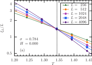
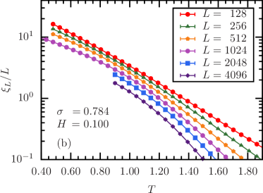
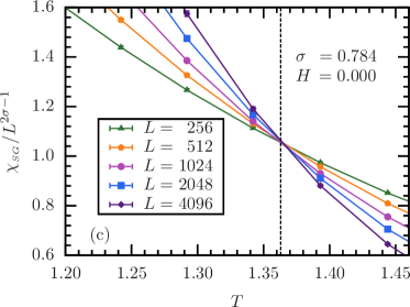
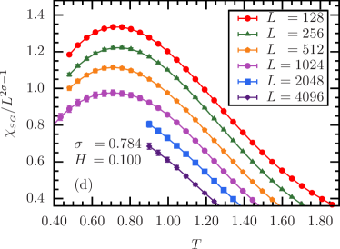
Figure 1: (Color online) Data used in a standard FSS for $\sigma=0.784$, which is a proxy for four dimensions. The left column is for $H=0$ and the right column for $H=0.1$. The top row shows the finite-size correlation length divided by $L$ as a function of temperature $T$ for different system sizes. The bottom row shows results for the scale-invariant spin-glass susceptibility, $\chi_{{}_{\rm SG}}/L^{2\sigma-1}$. The intersections seen in the left-hand column indicate a transition in zero field. The intersection temperatures (shown by the dashed vertical line) are $T_{c}\simeq 1.34$ from $\xi_{L}/L$ data in (a), and $T_{c}\simeq 1.36$ from $\chi_{\rm SG}/L^{2\sigma-1}$ data in (c). The small difference is likely due to sensitive corrections to scaling in the susceptibility (see Ref. Katzgraber et al., 2006 for details). By contrast, the lack of intersections in the right-hand column indicates no transition in a magnetic field.

Both the correlation length in Eq. (7) and the spin-glass susceptibility in Eq. (8) involve $k=0$ fluctuations. Recently, Refs. Leuzzi et al., 2009, Leuzzi et al., 2011, and Baños et al., 2012b have argued that one should avoid data at $k=0$ for spin glasses in the presence of a magnetic field on the grounds that there are large corrections to FSS. We discuss this in detail below and for now just present the new proposed quantities to be measuredLeuzzi et al. (2009, 2011); Baños et al. (2012b) that avoid $k=0$ fluctuations. We shall use the term “modified” FSS analysis to denote the use of these quantities. Below we compare the results of this modified analysis with results obtained from Eqs. (7) and (8), which we denote the “standard” FSS approach.

At long wavelength one expects

$$\chi_{{}_{\rm SG}}(k)^{-1}=\chi_{{}_{\rm SG}}(0)^{-1}+By+Cy^{2}$$ (9)

with $y=k^{2\sigma-1}$, which is the generalization of the Ornstein-Zernicke equation to long-range interactions, so one can calculate $\chi_{{}_{\rm SG}}(0)^{-1}$ indirectly by fitting data for nonzero $k$ to this form. For $L\to\infty$, this extrapolated value, $\chi_{{}_{\rm SG}}(k\to 0)^{-1}$, vanishes at and below the transition temperature. Interestingly, one findsLeuzzi et al. (2009, 2011) that the extrapolated value goes through zero even for a finite system, at a temperature $T^{\star}(L)$ which tends to $T_{c}$ for $L\to\infty$. This means $T_{c}=\lim_{L\to\infty}T^{\star}(L)$. We find quite strong corrections to the asymptotic result (as found also for the Sherrington-Kirkpatrick model in Ref. Billoire and Coluzzi, 2003), so we include the leading correction to scaling by fitting the data to

$$T^{\star}(L)=T_{c}+{A\over L^{\lambda}},$$ (10)

where $\lambda$ is a correction to scaling exponent and $A$ is the amplitude of the correction.

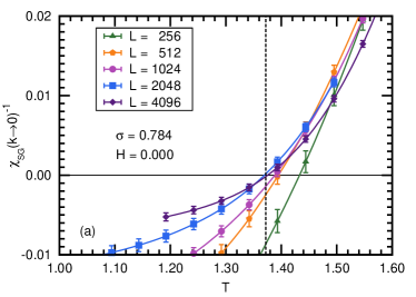
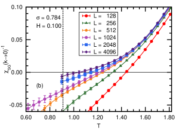
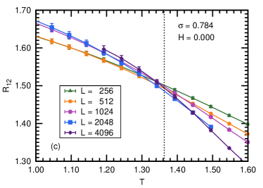
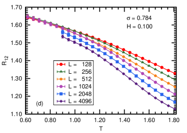
Figure 2: (Color online) Data used in the modified FSS analysis for $\sigma=0.784$. As in Fig. 1, the left column is for $H=0$ and the right column for $H=0.1$. The top row shows the inverse spin-glass susceptibility $\chi_{{}_{\rm SG}}(k\to 0)^{-1}$ extrapolated from results for $k\neq 0$. The bottom row shows data for the dimensionless ratio $R_{12}$ defined in Eq. (11). The dashed line for $\chi_{{}_{\rm SG}}(k\to 0)^{-1}$ [top row, panels (a) and (b)] indicates the extrapolated transition temperature $T_{c}$ determined from the fits in Fig. 3. The $R_{12}$ data for $H=0$ [panel (c)] show intersections but the trend of intersection temperatures is not smooth for this range of sizes. The dotted vertical line shows the transition temperature estimated from the intersections of $\chi_{{}_{\rm SG}}/L^{2\sigma-1}$ in Fig. 1 ($T_{c}=1.36$) and so is just a guide to the eye. The $R_{12}$ data for $H=0.1$ [panel (d)] show no sign of a transition in the range of temperatures studied.

This method requires several nonzero wave vectors and so is particularly suitable for one-dimensional models as studied here, because one can simulate very large linear sizes for these. For a short-range model in 4D, where the number of wave vectors is more limited, the authors of Ref. Baños et al., 2012b propose another quantity. To motivate this quantity, we note as stated above, that $\xi_{L}/L$ is particularly useful because it is dimensionless. From Eq. (6) we see that the crucial quantity is the ratio $\chi_{{}_{\rm SG}}(0)/\chi_{{}_{\rm SG}}(k_{1})$, which is also dimensionless. Massaging this quantity to obtain another dimensionless quantity $\xi_{L}/L$ according to Eq. (6) is actually not essential. Therefore, a related quantity which does not involve $k=0$ can be defined via

$$R_{12}={\chi_{{}_{\rm SG}}(k_{1})\over\chi_{{}_{\rm SG}}(k_{2})}\,,$$ (11)

where $k_{2}=4\pi/L$ is the second smallest nonzero wave vector. Because it is dimensionless, $R_{12}$ has the same FSS form as $\xi_{L}/L$ shown in Eq. (7). Consequently, curves of $R_{12}$ for different system sizes $L$ should intersect at $T_{c}$ if corrections to FSS are unimportant.

II.3 Numerical Details

The simulations are done using the parallel tempering (exchange) Monte Carlo method.Geyer (1991); Hukushima and Nemoto (1996) Simulation parameters are listed in Table 1. Equilibration is tested using the method developed in Ref. Katzgraber et al., 2009 [Eq. (8)]: The energy per spin is computed directly, as well as as a function of a spin correlator. Both have to agree if a system is in thermal equilibrium. Starting from a random configuration, the directly computed energy is typically overestimated, while the energy computed from the correlator is underestimated. Only when both agree (on average) is the system in thermal equilibrium. We thus perform a logarithmic binning of the data and requiring that both the energy per spin and the energy computer from the correlator agree for at least the last two logarithmic bins. The reason we wait for two additional logarithmic bins is because the equality only holds on average. By being more conservative with the equilibration times we ensure that the bulk of the samples are in thermal equilibrium.Yucesoy et al. (2013) In addition, we verify that all other observables are independent of Monte Carlo time for at least these last two bins.

III Results

III.1 $\boldsymbol{\sigma=0.784}$ (four space dimensions)

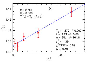
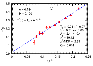
Figure 3: (Color online) Values of $T^{\star}(L)$, the temperature where $\chi_{{}_{\rm SG}}(k\to 0)^{-1}$ goes through zero, for different system sizes for $H=0$ (left) and $H=0.1$ (right) for $\sigma=0.784$. The data are fitted to Eq. (10) with $T_{c}$, $A$, and $\lambda$ as adjustable parameters. In both cases a finite value of $T_{c}$ (the intercept) is found. For $H=0$ the goodness-of-fit parameterQ ; Press et al. (1992) $Q$ is not very small, indicating a satisfactory fit. For $H=0.1$ the value of $Q$ is smaller because the point for the largest size is well below the fit.

When $\sigma=0.784$ the one-dimensional model is a proxy for a short-range model in four space dimensions. Data for $\xi_{L}/L$ and $\chi_{{}_{\rm SG}}/L^{2\sigma-1}$, used within the standard FSS, are shown in Fig. 1 for $H=0$ (left column) and $H=0.1$ (right column). The zero-field data for the scaled $\chi_{{}_{\rm SG}}$ in Fig. 1(c) show clear intersections indicating a transition at $T_{c}\simeq 1.36$, while the data for $\xi_{L}/L$ in Fig. 1(a) show clear intersections at $T_{c}\simeq 1.34$. This (small) difference is presumably due to corrections to scaling. Because there is no doubt that there is a zero-field transition for the models studied in this paper (see e.g., Ref. Baños et al., 2012a) we have not carried out a precise estimate of the value of $T_{c}$ in zero field.

In contrast to the zero-field data, the data in a field of $H=0.1$, Figs. 1(b) and 1(d), show no intersections, indicating the absence of a transition, at least for this range of temperatures and field.

Data for the extrapolated value of $\chi_{{}_{\rm SG}}(k\to 0)^{-1}$ fitted according to Eq. (9) and $R_{12}$ defined via Eq. (11) are shown in Fig. 2 and used in the modified FSS. The zero-field data for $R_{12}$ in Fig. 2(c) show intersections but the intersection temperatures do not vary monotonically for this range of sizes. The dotted vertical line in Fig. 2(c) corresponds to $T_{c}$ from the scaled $\chi_{{}_{\rm SG}}$ data in Fig. (1)(c), and so is only a guide to the eye. The data for $R_{12}$ in a field ($H=0.1$) in Fig. 2(d) have no intersections, i.e., no transition is visible for the range of temperatures studied.

For each system size, the temperature where the data for $\chi_{{}_{\rm SG}}(k\to 0)^{-1}$ shown in Figs. 2(a) and  2(b) goes through zero is referred to as $T^{\star}(L)$. This value is obtained by fitting the data to a cubic polynomial (using the seven data points nearest to zero), and error bars are obtained from a bootstrap analysis. The results are shown in Fig. 3. The thermodynamic transition temperature $T_{c}$ is then given by $\lim_{L\to\infty}T^{\star}(L)$, which we estimate by fitting to Eq. (10). The fits, obtained by adjusting $T_{c}$, $A$, and $\lambda$, are shown in the figures (dashed lines). The data indicate a finite value of $T_{c}$ both in a field and in zero field. The central values for $T_{c}$ are shown by the dashed vertical lines in Figs. 2(a) and 2(b). The value of $\chi^{2}/N_{\text{DOF}}$, where $N_{\text{DOF}}$ is the number of degrees of freedom and the goodness-of-fit parameterQ ; Press et al. (1992) $Q$, indicate a good fit in the case of $H=0$ ($Q=0.50$). For $H=0.1$, the value of $Q$ is smaller ($Q=0.014$) because the point for the largest size is well below the fit.

Our analysis to ascertain whether there is a finite $T_{c}$ includes four sets of data: $\xi_{L}/L$, $\chi_{{}_{\rm SG}}/L^{2\sigma-1}$, $\chi_{{}_{\rm SG}}(k\to 0)^{-1}$, and $R_{12}$. In zero field they all clearly show a finite transition temperature, in agreement with the work of Baños et al.Baños et al. (2012a), who studied almost the same model. However, in a field of $H=0.1$ there is an inconsistency: Three of the four measures ($\xi_{L}/L$, $\chi_{{}_{\rm SG}}/L^{2\sigma-1}$, and $R_{12}$) show no sign of a transition. In contrast, the value of $T_{c}$ from results for $\chi_{{}_{\rm SG}}(k\to 0)^{-1}$ does appear to be nonzero ($T_{c}=0.91\pm 0.07$), see Fig. 3(b). We note, however, that the error bar is large and the last data point being below the fit may possibly indicate a downward trend at larger sizes.

This discrepancy highlights the need to better understand FSS in spin glasses in a magnetic field. We shall come back to this question in Sec. IV. However, already we note that because the $\chi_{{}_{\rm SG}}(k\to 0)^{-1}$ data are the only indicator for a finite $T_{c}$ in a field, we feel we should view results for this quantity with caution.

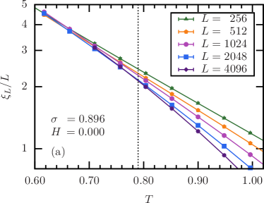
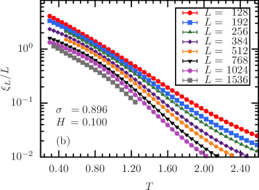
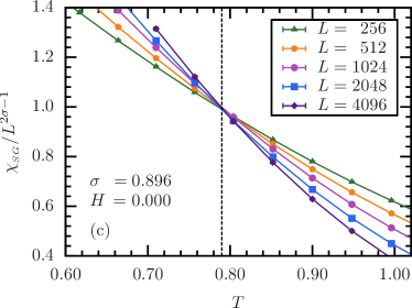
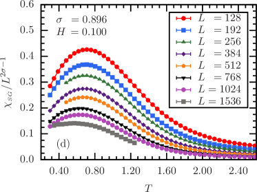
Figure 4: (Color online) Data used in the standard FSS for $\sigma=0.896$, which is a proxy for three space dimensions. The left column is for $H=0$ and the right column for $H=0.1$. The top row shows the finite-size correlation length divided by $L$ as a function of $T$ for different system sizes. The bottom row shows results for the scale-invariant spin-glass susceptibility, $\chi_{{}_{\rm SG}}/L^{2\sigma-1}$. The intersections in the data for $\chi_{{}_{\rm SG}}/L^{2\sigma-1}$ for $H=0$ [panel (c)] indicate a transition at $T_{c}\simeq 0.795$, which is shown by a dashed vertical line. The zero-field results for $\xi_{L}/L$ [panel (a)] show stronger finite-size effects and the evidence for intersections is not so clear. The same result was found recently by Baños et al.Baños et al. (2012a), who were able to study somewhat larger sizes for almost the same model. Their FSS analysis of all their data supports a zero-field transition. In panel (a) the dotted vertical line indicates the transition temperature found for the data in panel (c) and so is just a guide to the eye. The data in panel (a) are consistent with intersections tending to this value for $L\to\infty$. By contrast, the lack of intersections in the right-hand column indicates no transition in a magnetic field.

III.2 $\boldsymbol{\sigma=0.896}$ (three space dimensions)

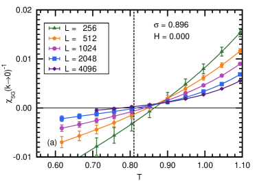
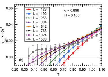
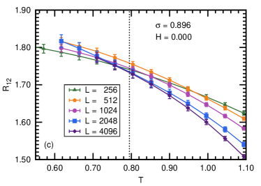
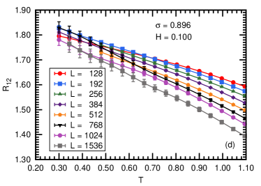
Figure 5: (Color online) Data used in the modified FSS analysis for $\sigma=0.896$. As in Fig. 4, the left column is for $H=0$ and the right column for $H=0.1$. The top row shows the inverse spin-glass susceptibility $\chi_{{}_{\rm SG}}(k\to 0)$ extrapolated from results for $k\neq 0$. The bottom row shows data for the dimensionless ratio $R_{12}$ defined in Eq. (11). The dashed vertical line in panel (a) marks the value for $T_{c}$ obtained by extrapolating the data for $T^{\star}(L)$ [where $\chi_{{}_{\rm SG}}(k\to 0)^{-1}$ vanishes] according to Eq. (10); see Fig. 6. The result is $T_{c}=0.81(3)$, in agreement with the value of $0.795$ from the intersections of the scaled $\chi_{{}_{\rm SG}}$ in Fig. 4(c). The data for $R_{12}$ in zero field in panel (c) show intersections, although the intersection temperatures do not vary smoothly. The dotted vertical line shows $T_{c}$ obtained from the scaled $\chi_{{}_{\rm SG}}$ and is just a guide to the eye. The results for $R_{12}$ for $H=0.1$ in panel (d) do not provide clear evidence for a transition.

The one-dimensional long-range model with $\sigma=0.896$ is a proxy for a short-range spin glass in three space dimensions. The data used in the standard FSS analysis are shown in Fig. 4. Again, the left column is for $H=0$ and the right column is for $H=0.1$. The zero-field results for the scaled $\chi_{{}_{\rm SG}}$ in Fig. 4(c) show a clear transition. The zero-field data for $\xi_{L}/L$ in Fig. 4(a) are less clear cut because there is little splaying of the data at low temperatures. However, the temperature where the data merge for two neighboring sizes increases as the system size increases. Similar results were obtained by Baños et al.Baños et al. (2012a) for almost the same model, although they were able to study sizes of up to $L=8192$ which do show a clear intersection with the data for $L=4096$ (see Fig. 15 in their paper). Performing a detailed FSS analysis, Baños et al.Baños et al. (2012a) showed that all their data are consistent with a finite value of $T_{c}$. Because our data for $\xi_{L}/L$ do not in itself convincingly locate the transition temperature, the dotted line in Fig. 4(a) shows (as a guide to the eye) the location of $T_{c}$ as determined from the scaled $\chi_{{}_{\rm SG}}$ data in Fig. 4(c).

In a field, the data for $\xi_{L}/L$ in Fig. 4(b) and the scaled spin-glass susceptibility in Fig. 4(d) show no intersections and, hence, indicate that there is no transition for this range of temperature and field.

Data for the modified FSS analysis are shown in Fig. 5. The results for $R_{12}$ are shown in the bottom row. In zero field [see Fig. 5(c)] there are clear intersections, although these do not vary monotonically for the range of sizes studied. However, the data are consistent with the value $T_{c}\simeq 0.795$ obtained from the scaled $\chi_{{}_{\rm SG}}$ data in Fig. 4(c), and this value is indicated as a guide to the eye by the dotted vertical line in Fig. 5(c). The data for $R_{12}$ in a field $H=0.1$ [Fig. 5(d)] do not show clear evidence for a transition in the range of temperatures studied.

The top row of Fig. 5 shows results for $\chi_{{}_{\rm SG}}(k\to 0)^{-1}$. The temperatures where $\chi_{{}_{\rm SG}}(k\to 0)^{-1}=0$ are plotted and fitted according to Eq. (10) in Fig. 6. The values of $Q$, $0.37$ for $H=0$ and $0.91$ for $H=0.1$, indicate a good fit. For $H=0$ the result is $T_{c}=0.81\pm 0.03$ and the central value is indicated by the dashed vertical line in Fig. 5(a). This value is consistent with the value $0.795$ from the data for the scaled $\chi_{{}_{\rm SG}}$ in Fig. 4(c). For $H=0.1$, the values of $T^{\star}(L)$ shown in Fig. 6(b) have a very strong size dependence. The figure also shows the values of the parameters obtained by fitting the data to Eq. (10). In particular, we find $T_{c}=-0.37\pm 1.15$, indicating that the optimal $T_{c}$ is negative but the error bar is very large. This large error bar requires more discussion, which we now give.

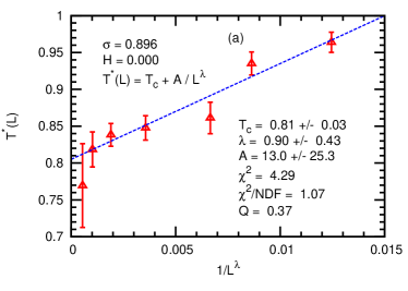
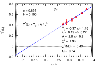
Figure 6: (Color online) Values of $T^{\star}(L)$, the temperature where $\chi_{{}_{\rm SG}}(k\to 0)^{-1}$ goes through zero, for different system sizes for $H=0$ (left) and $H=0.1$ (right) for $\sigma=0.896$. The data are fitted to Eq. (10) with $T_{c}$, $A$, and $\lambda$ as adjustable parameters. The error bars on the parameters in the fit to the $H=0.1$ data are very large (this is discussed in the text and in the caption to Fig. 8). Note that the $H=0.1$ data are consistent with $T_{c}=0$. The goodness-of-fit parameterPress et al. (1992) indicates a satisfactory fit in both cases.

First, we note that a log-log plot of the data in Fig. 7 indicates that the data are compatible with $T_{c}=0$. In addition, we perform the following analysis: For each system size we construct $200$ bootstrap data sets and estimate $T^{\star}(L)$ for each of them. There is a huge scatter in the estimates from the largest size $L=1536$. Thus we ignore this size in the analysis. For $L=784$, $9$ of the $200$ bootstrap data sets do not yield a temperature where $\chi_{\rm SG}(k\to 0)^{-1}$ vanishes. Hence, we consider $191$ bootstrap data sets and fit each of them according to Eq. (10).

Figure 8 shows the resulting cumulative distribution of transition temperatures, i.e., the probability that the transition temperature is less than the stated value. We find that $34$ of the $191$ data sets do not have a minimum in $\chi^{2}$; rather, considering $\chi^{2}$ as a function of $T_{c}$ while optimizing with respect to the other fit parameters, $\chi^{2}$ decreases monotonically as $T_{c}\to-\infty$ while $\lambda\to 0$ in this limit. The estimate of $T_{c}$ from the global fit ($T_{c}=-0.37$, indicated by the dashed vertical line) agrees well with the median (50th percentile) of the bootstrap estimates. The median is indicated by a horizontal dashed line. Also indicated by horizontal dashed lines are the 16th and 84th percentiles, which would correspond to one standard deviation if the distribution of $T_{c}$’s were Gaussian, which is clearly not the case here. Only 30% of the bootstrap fits have a positive $T_{c}$. We therefore conclude that a positive $T_{c}$ is somewhat unlikely but cannot be completely excluded by the data for $T^{\star}(L)$.

To conclude this subsection, all data are consistent with there being no AT line at $H=0.1$ for $\sigma=0.896$. The results for $T^{\star}(L)$ obtained from the vanishing of $\chi_{{}_{\rm SG}}(k\to 0)^{-1}$ do not exclude a finite $T_{c}$, but this possibility does not seem to be supported by the rest of the data.

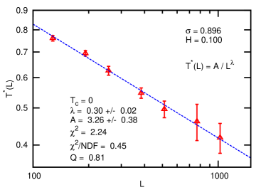
Figure 7: (Color online) Log-log plot of the data for $T^{\star}(L)$ for $\sigma=0.896$ and $H=0.1$ assuming $T_{c}=0$. The fit works very well according to the goodness-of-fit parameter $Q$, which is $0.81$.

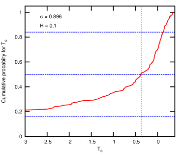
Figure 8: (Color online) Cumulative distribution of the transition temperature $T_{c}$ obtained from a bootstrap analysis of the data for $\sigma=0.896$ and $H=0.1$. The estimate of $T_{c}$ from the global fit ($T_{c}=-0.37$, indicated by the dashed vertical line) agrees well with the median (50th percentile) of the bootstrap estimates, which is indicated by a horizontal dashed line. Also indicated by horizontal dashed lines are the 16th and 84th percentiles which would correspond to one standard deviation if the distribution of $T_{c}$’s were Gaussian, which is clearly not the case. Only 30% of the bootstrap fits have a positive $T_{c}$.

IV Conclusions

We have presented results of simulations of one-dimensional spin-glass models in a magnetic field which are proxies for short-range models in three and four space dimensions. We have analyzed the results using both a traditional FSS approach (which uses $k=0$ data) and a recently proposed modified FSS approach which uses only $k>0$ data.

For the model which is a proxy for a 3D system, all our results are consistent with there being no transition in a magnetic field, at least for the range of fields and temperatures that we can study. The results for $T^{\star}(L)$, obtained from the modified FSS analysis, are just compatible with a finite $T_{c}$ but the other data are only compatible with the absence of a transition, at least assuming that the data are in the asymptotic scaling region.

For the model which is a proxy for a 4D system, three of the four sets of data indicate the absence of a transition in a field ($\xi_{L}/L$, $\chi_{{}_{\rm SG}}/L^{2\sigma-1}$, and $R_{12}$), while that for $T^{\star}(L)$ gives a satisfactory fit indicating $T_{c}>0$. This contradiction indicates that at least some of the data cannot be in the asymptotic scaling region.

It is, therefore, crucial to understand whether it is better to use $k=0$ data in the analysis as in the standard approach or to exclude that data as in the modified approach.Leuzzi et al. (2009, 2011); Baños et al. (2012b) References Leuzzi et al., 2009, Leuzzi et al., 2011, and Baños et al., 2012b argue that the $k=0$ data have strong corrections to FSS. On the other hand, the divergence occurs at $k=0$ and normally one uses divergent quantities in FSS because these should show the asymptotic FSS behavior for the smaller system sizes. It should also be noted that Ref. Jörg et al., 2008 found good agreement for the location of the AT line for the spin glass on a random graph, i.e., the Viana-Bray model (which corresponds to the $\sigma=0$ limit of the present model), using the scaled $\chi_{{}_{\rm SG}}$, i.e., the $k=0$ fluctuations.

Finally, an alternate interpretation of the results can be done using droplet scaling arguments.Fisher and Huse (1987, 1988); Bray and Moore (1986); McMillan (1984) The size $\xi_{\rm D}$ of the droplets within this picture can be estimated by equating the domain-wall energy required to create them, $\sim J\xi_{\rm D}^{\theta}$, to the energy which can be gained from flipping a droplet of size $\xi_{\rm D}$ in the field, $\sim H\xi_{\rm D}^{d/2}$, where $d$ is the space dimension. For the long-range models studied here, $\theta=1-\sigma$.Katzgraber and Young (2003) Thus, the droplet size is of order $3320$ for $\sigma=0.784$ and is of order $335$ at $\sigma=0.896$, when $H/J=0.1$, the ratio used in this study. We have only one data point, that for $L=4096$ in Fig. 6(b), greater than $3320$. Interestingly, it is the data points at the smaller values of $L$ which point to a finite value of $T_{c}$. The last point at system size $4096$ lies well below the fitted curve. This suggests that had we been able to obtain data for a range of system sizes significantly greater than $4096$, it might have been possible to obtain results in the analog of four dimensions like that displayed in Fig. 7 for the analog of three dimensions, where the last five data points are all greater than the estimated droplet size there of $335$ and the extrapolated value of $T_{c}$ is zero.

Ideally, one would determine which set of data is in the asymptotic scaling regime by simulating larger system sizes. However, because the present study involved a rather substantial amount of CPU time, this is not feasible for us at present. Based on the data shown, the balance of the evidence is that there is no AT line in the one-dimensional models which are proxies for three and four dimensional short-range spin glasses. However, a deeper insight into corrections to FSS in spin glasses is needed to confirm this conclusion.