3D hydrodynamical CO⁵BOLD model atmospheres of red giant stars

Abstract

Context. Red giant stars are important tracers of stellar populations in the Galaxy and beyond, thus accurate modeling of their structure and related observable properties is of great importance. Three-dimensional (3D) hydrodynamical stellar atmosphere models offer a new level of realism in the modeling of red giant atmospheres but still need to be established as standard tools.

Aims. We investigate the character and role of convection in the atmosphere of a prototypical red giant located close to the red giant branch (RGB) tip with atmospheric parameters, $T_{\rm eff}=3660$ K, $\log g=1.0$, $[\mathrm{M/H}]=0.0$.

Methods. Differential analysis of the atmospheric structures is performed using the 3D hydrodynamical and 1D classical atmosphere models calculated with the CO⁵BOLD and LHD codes, respectively. All models share identical atmospheric parameters, elemental composition, opacities and equation-of-state.

Results. We find that the atmosphere of this particular red giant consists of two rather distinct regions: the lower atmosphere dominated by convective motions and the upper atmosphere dominated by wave activity. Convective motions form a prominent granulation pattern with an intensity contrast ($\sim 18\%$) which is larger than in the solar models ($\sim 15\%$). The upper atmosphere is frequently traversed by fast shock waves, with vertical and horizontal velocities of up to Mach $\sim 2.5$ and $\sim 6.0$, respectively. The typical diameter of the granules amounts to $\sim 5$ Gm which translates into $\sim 400$ granules covering the whole stellar surface. The turbulent pressure in the giant model contributes up to $\sim 35\%$ to the total (i.e., gas plus turbulent) pressure which shows that it cannot be neglected in stellar atmosphere and evolutionary modeling. However, there exists no combination of the mixing-length parameter, $\alpha_{\mathrm{MLT}}$, and turbulent pressure, $P_{\rm turb}$, that would allow to satisfactorily reproduce the 3D temperature-pressure profile with 1D atmosphere models based on a standard formulation of mixing-length theory.

1 Introduction

Convection plays an important role in governing the interior structure and evolution of red giants (i.e., stars on the red and asymptotic giant branches, RGB/AGB). Besides of aiding the energy transport from the stellar interior to the outer layers, convection mixes heavy elements from the nuclear burning layers up into the stellar envelope and atmosphere. Since convective mixing changes the local chemical composition it alters the stellar structure because of changes in the opacities, thermodynamic properties, and nuclear reaction rates of the stellar plasma. This affects the observable properties of a star, and a proper understanding of convection is thus of fundamental importance for building realistic models for stellar structure and evolution, which, in turn, are fundamental building blocks of our understanding of individual stars and stellar populations.

Convection in current one-dimensional (1D) hydrostatic stellar atmosphere models is treated in a simplified way, typically, using the classical mixing-length theory (MLT, Böhm-Vitense, 1958) or one of its more advanced variants (Canuto & Mazzitelli, 1991; Canuto et al., 1996). This approach has a number of drawbacks. For instance, the efficiency of convective transport in the framework of MLT is scaled by the apriori unknown mixing-length parameter, $\alpha_{\mathrm{MLT}}$. It is commonly taken as a fixed ratio of the mixing-length to the local pressure scale height, and is usually calibrated using theoretical models of the Sun. Since the MLT is a rather simplistic approach, $\alpha_{\mathrm{MLT}}$ needs not to be the same in main-sequence stars, subgiants, giants and supergiants, as is normally assumed in the calculation of stellar atmosphere models (Castelli & Kurucz, 2003; Brott & Hauschildt, 2005; Gustafsson et al., 2008) or stellar evolutionary tracks and isochrones (Demarque et al., 2004; Vandenberg et al., 2006; Dotter et al., 2008; Bertelli et al., 2008, 2009).

Despite significant efforts made during the last few decades to improve the treatment of convection in stellar structure models a fundamental breakthrough is still missing. Seeking numerical solutions of the underlying radiation-hydrodynamical equations is a promising way to make progress since such models lay-out a clear path towards increasing realism in the description of convection. In this class of models three-dimensional (3D) hydrodynamical model atmospheres have already demonstrated their excellent capabilities of reproducing the observed properties of surface convection in the Sun (e.g., Stein & Nordlund, 1998), and associated spectral diagnostics (e.g., Asplund et al., 2000; Caffau et al., 2008, 2010), in many cases outperforming classical 1D models despite lacking tunable parameters as in 1D. Similarly successfully, such 3D models were applied to other types of stars, such as late-type dwarfs (González Hernández et al., 2009; Ramírez et al., 2009; Behara et al., 2010) and subgiants (Collet et al., 2009).

The progress in the 3D modeling of red giant atmospheres has been considerably slower. To large extent this is related to the fact that giant models are computationally more demanding, and the calculation of a grid of giant atmosphere models is a sizable task. Among the early efforts, a 3D model atmosphere of a red giant was discussed by Kučinskas et al. (2005). The authors have compared broad band photometric colors as predicted by the classical 1D and 3D hydrodynamical model atmospheres and have shown that for certain color indices the 3D–1D differences may reach $\sim$ 0.25 mag. A detailed analysis of the spectral line formation in the atmospheres of somewhat warmer red giants ($T_{\mathrm{eff}}\approx 4700-5100$ K, $\log g=2.2$, $[\mathrm{M/H}]=0.0$ to $-3.0$) was carried out by Collet et al. (2007). An interesting finding of this work is that convective motions may produce significantly cooler average temperatures in the outer atmospheric layers, an effect which is increasingly pronounced at low metallicities ($[\mathrm{Fe/H}]<-2.0$). Similar effects have been seen in the 3D atmosphere models of late-type dwarfs too, see, e.g., Asplund et al. (1999), Behara et al. (2010), González Hernández et al. (2010). Spectral lines of various atoms and molecules appear typically stronger in a 3D than in a 1D model which leads to a disagreement between the chemical abundances, $\epsilon(X)$, reaching $\Delta\log\epsilon(X)=-0.5\dots\ -1.0$ dex at the lowest metallicities. Despite these successful attempts, 3D hydrodynamical model atmospheres of red giants still need to be consolidated including comparisons to observations as exemplified by Ramírez et al. (2010) who performed a study of a metal-poor giant with emphasis on hydrodynamic properties.

To further broaden the 3D model basis of giants, we undertook a study of the influence of convection on the structure and observable properties of red giants. The models were calculated with the 3D radiation-hydrodynamics code CO⁵BOLD and will eventually cover the entire range of stellar parameters typical for stars on the red and asymptotic giant branches (RGB and AGB, respectively). Some of these models are already available as part of the CIFIST grid of CO⁵BOLD 3D model atmospheres (Ludwig et al., 2009). This homogeneous set of 3D model atmospheres is well suited to investigate the role of convection in the atmospheres of red giants of different effective temperatures, gravities and metallicities.

This paper summarizes the first results of the project, focusing on the role of convection shaping the atmospheric structure of a solar-metallicity red giant located close to the RGB tip. The atmospheric parameters of the model are $T_{\mathrm{eff}}$=3660 K, $\log g$=1.0, $\left[\mathrm{M}/\mathrm{H}\right]$=0.0. The analysis is done differentially by comparing 3D hydrodynamical and 1D static model atmospheres calculated for the same set of atmospheric parameters and with identical opacities and equation-of-state. In two companion papers we will further discuss the effects of convection on the observable properties of this particular red giant, by taking a closer look at the formation of individual spectral lines and global properties of the spectral energy distribution (Kučinskas et al. 2012a,b , in prep.) The present paper mostly describes morphological properties of the particular model which we, however, generalize in places to make statements about convection in red giants in general.

2 The model setup

Figure 1: Snapshots of the emergent white light intensity during the temporal evolution (ordered upper-left to lower-right) of the hydrodynamical red giant model atmosphere. Bright granules where the matter is rising are surrounded by darker and significantly narrower intergranular lanes associated with down-flows. The spatial size of each frame is 15.6$\times$15.6 Gm², and the time interval between frames 300 ks. The relative RMS intensity contrast is given in the upper left corner of each frame.

Two stellar atmosphere models were used in this study to assess the influence of convection on the atmospheric structures of a red giant: 3D hydrodynamical and classical 1D models, calculated with the codes CO⁵BOLD and LHD, respectively. Both models were computed using identical atmospheric parameters, $T_{\mathrm{eff}}\approx 3660$ K, $\log g=1.0$, $[\mathrm{M/H}]=0.0$. According to theoretical evolutionary tracks (e.g., Cordier et al., 2007) this set of atmospheric parameters characterizes a late-type giant located close to the RGB tip, with a mass of $\sim$ 2 ${\rm M_{\odot}}$ and age of $\sim$ 1 Gyr. In turn, the mass and gravity give a radius of $\sim\,75\,{\rm R_{\odot}}$.

2.1 The 3D CO⁵BOLD model

The 3D atmosphere model was calculated using the CO⁵BOLD stellar atmosphere code. The CO⁵BOLD code employs a Riemann solver of Roe type to integrate the equations of hydrodynamics and simultaneously solve for the frequency-dependent radiation field on a 3D Cartesian grid (Freytag et al., 2002, 2003; Wedemeyer et al., 2004; Freytag et al., 2010). For a detailed description of the code and its applications see Freytag et al. (2012).

The code was employed in the ’box-in-a-star’ set-up using a grid of $150\times 150\times 151$ mesh points ($x\times y\times z$, where $z$ is vertical dimension), with a corresponding size of the computational domain of $15.6\times 15.6\times 8.6$ Gm³. Effects related to the stellar sphericity are neglected. We applied open boundary conditions in the vertical direction and periodic boundaries in the horizontal direction. The convective flux at the lower boundary was controlled by specifying the entropy of the inflowing gas. The model spans a range in optical depth of $-6.5\lesssim\log\,\langle\tau_{\rm Ross}\rangle\lesssim 5$ and samples the atmospheric layers over $\sim$11 pressure scale heights.

In the model calculations we used monochromatic opacities from the MARCS stellar atmosphere package (Gustafsson et al., 2008), grouped into 5 opacity bins (for more on opacity grouping scheme see Nordlund, 1982; Ludwig, 1992; Ludwig et al., 1994; Vögler, 2004). Opacities were calculated assuming solar elemental abundances according to Grevesse & Sauval (1998), with the exception of carbon, nitrogen and oxygen, for which the following values were used: A(C)=8.41, A(N)=7.8, A(O)=8.67, similar to the CNO abundances recommended by Asplund et al. (2005). Local thermodynamical equilibrium (LTE) was assumed throughout the entire atmosphere and scattering was treated as true absorption.

The equation-of-state (EOS) used in the model simulations takes into account the ionization of hydrogen and helium, as well as formation of H₂ molecules according to Saha-Boltzmann statistics. The ionization of metals is ignored in the current version of EOS since its importance for the gross thermodynamical properties is minor.

After initial relaxation to a quasi-stationary state, the model simulations were run to cover a span of $\sim 6\times 10^{6}$ sec ($\sim 70$ days) in stellar time. This corresponds to $\sim 7$ convective turnover times as measured by the Brunt-Väisälä and/or advection timescales, the latter equal to the time needed by the convective material to cross one mixing-length, $\Lambda\equiv\alpha_{\rm MLT}H_{\rm p}$, where $H_{\rm p}$ is the pressure scale height (both timescales were estimated at $\tau_{\rm Ross}=1.0$, see Sect. 3.2.3). A set of 70 relaxed 3D model snapshots was used in our analysis of the atmospheric structure. This is sufficient for the aspects addressed in this work. However, one should keep in mind that the overall statistics gathered is limited (in part dictated by computational cost), and the precision of convection-related properties (e.g., the turbulent pressure) is likely not better than $\sim 5\,\%$.

2.2 The average $\left\langle\mbox{3D}\right\rangle$ CO⁵BOLD model

Since the 3D hydrodynamical and 1D classical model atmospheres are based on different physical assumptions, one may naturally expect differences in their resulting properties. Two aspects are worth mentioning here. First, the 3D hydrodynamical model atmospheres predict significant horizontal fluctuations in temperature, density, pressure, velocity and other kinematic and thermodynamic properties. This may produce horizontal variations in, e.g., shapes and strengths of spectral lines formed in different parts of the model photosphere. Second, convection is a natural process arising in hydrodynamical model atmospheres inherent to the equations of hydrodynamics and radiative transfer. Besides convection as such, hydrodynamical models exhibit significant overshoot of material into the upper layers of the atmosphere which should be convectively stable under the Schwarzschild criterium. None of these effects is properly accounted for in the 1D classical models built on the prescription given by MLT. The consequence is that the structure of 3D hydrodynamical models, even if horizontally averaged, is different from 1D models calculated with identical atmospheric parameters.

The relative importance of these effects can be assessed using the average 3D model. Such a model can be calculated by horizontally averaging the thermal structure over several instances in time (snapshots). By definition, the new one-dimensional structure, further referred to as $\left\langle\mbox{3D}\right\rangle$ model, retains no information about the horizontal inhomogeneities but keeps the imprints from the different (i.e., hydrodynamical) treatment of convection in the original 3D model. The 3D–$\left\langle\mbox{3D}\right\rangle$ and $\left\langle\mbox{3D}\right\rangle$–1D differences may therefore provide valuable information about the relative importance of horizontal fluctuations and the time-dependent effects related with the treatment of convection, respectively.

The $\left\langle\mbox{3D}\right\rangle$ model used in this work was obtained by averaging 70 3D snapshots over the surfaces of equal Rosseland optical depth. To preserve the radiative properties of the original 3D model we averaged the fourth moment of temperature and first moment of gas pressure, following the prescription given in Steffen et al. (1995).

2.3 1D LHD model

Comparison 1D hydrostatic models were calculated with the LHD code, using the same atmospheric parameters, elemental abundances, opacities and EOS as in the 3D model calculations described above. Convection in the LHD models is described using the mixing-length theory, adopting the formulation of Mihalas (1978). The LHD models characterized by several different mixing-length parameters were used in this work, with $\alpha_{\mathrm{MLT}}=1.0,1.5$ and 2.0. It should be stressed though that the choice of the mixing-length parameter affects mostly the deeper atmospheric layers and has limited influence on the formation of the emitted spectrum in this particular red giant (Kučinskas et al., 2005, Kučinskas et al. 2012, submitted to A&A).

In a few cases we added an ad-hoc overshooting in the LHD models. This was done by preventing the convective velocity going to zero in the formally stable regions but forcing it to a prescribed, fixed value. The convective flux was calculated from the standard MLT formulae. In the overshoot region this results in a downward directed convective flux, and usually a flux divergence which leads to additional cooling. This is intended to mimic the cooling effect by overshooting often observed in 3D models in the upper photosphere.

3 Results and discussion

3.1 Properties of surface granulation

Figure 2: Non-normalized probability density of the emergent white light intensity extracted from 14 snapshots of the 3D model. “all” labels the overall distribution, “up” and “down” are the distributions restricted to up- or down-flowing material only. Intensities are given as relative deviation from the (temporal and spatial) mean intensity. As velocity criterion the sign of the vertical velocity component at $\log\tau_{\mathrm{ross}}=0$ was taken.

The 3D model of red giant predicts the existence of surface granulation which is clearly visible in the time series of emergent white light intensities shown in Fig. 1. Although similar granulation patterns are routinely seen in the 3D models of the Sun (Nordlund, 1982), M-dwarfs (Ludwig et al., 2002), white dwarfs (Freytag et al., 1996), brown dwarfs (Freytag et al., 2010), pre-main sequence stars (Ludwig et al., 2006), subgiants (Ludwig et al., 2006) and warm giants (Collet et al., 2007), the existence of granulation in cool red giants is not exactly self-evident: MLT predicts that the surface convective zone is confined to optically thick layers in the 1D models of giants, with an only thin, marginally unstable region extending into the upper atmosphere (see the 1D stratification of the convective velocity in Fig. 10). Consequently, the outer optically thin regions are essentially unaffected by convection in 1D models.

In the 3D model, the geometric distance between the upper boundary of the convective region and the optically thin region is, however, not large. The material, therefore, crosses the formal boundary of the convective region and overshoots into the upper atmospheric layers. Similarly to dwarfs, the efficiency of convective overshoot exhibits an exponential decline with height, e.g., as hinted at by the shape of the vertical velocity profile in the optical depth range $\log\tau_{\rm Ross}\sim 1.0\dots-2.0$ (Fig. 10). According to Freytag et al. (1996), such exponential decline is caused by the penetration of convective modes with long horizontal wavelengths into the formally convectively stable layers.

It may perhaps be interesting to note that intergranular lanes are narrower in our giant model than those seen in the 3D models of the Sun but wider than in the models of late-type dwarfs (cf. Ludwig et al., 2006). Why this is so is not immediately clear, although the increase of the relative width of down-drafts with $T_{\mathrm{eff}}$ suggests that it may be related to a stronger smoothing of thermal inhomogeneities caused by the more intense radiative energy exchange at higher temperatures.

Figure 3: Emerging white light intensity (top panels), vertical ($v_{\rm z}$) and horizontal ($v_{\rm h}=\sqrt{v_{\rm x}^{2}+v_{\rm y}^{2}}$) velocities (bottom panels) in a typical 3D snapshot of the red giant model, all at $\log\tau_{\rm Ross}=0$. Yellow (bright) and brown (dark) pixels in the top-right and bottom panels highlight the areas where the relative intensity deviation is larger than $\Delta I/\langle I\rangle=0.3$ in the up-flows and down-flows, respectively. Locations where the vertical velocity $v_{\rm z}<-1$ Mach (supersonic down-flows) are marked with white contours, those where the vertical and horizontal velocities exceed 1 Mach are contoured in black (contours start at ${\rm Mach}=\pm 1.0$ and continue at $\pm 0.5$ Mach thereof). The relative white light intensity contrast is 18.2 % for this particular snapshot.

Despite the fact that the granulation pattern shown in Fig. 1 exhibits the typical appearance known from the 3D model atmospheres of other types of stars, Fig. 2 illustrates that its intensity distribution does not show the familiar bimodal shape related to the dark and bright areas of the granulation pattern but a single maximum. The intensity distributions restricted to up- and down-flowing regions makes it clear that the correlation between hot up-flowing and cool down-flowing gas is still present, a clear indication that convection as such takes place.

However, the intensity distributions in Fig. 2 illustrate that this correlation is far from perfect. For instance, high surface brightness does not necessarily imply that matter is in the up-flow since some of the down-flows may also be very bright. As seen in Fig. 3, such bright down-flows are typically seen on the edges of convective cells and in many cases are located immediately next to the uprising material that is also characterized by high white light intensities. The high intensity in these regions is caused by their significantly higher temperatures (see Fig. 5). These are, in turn, caused by the dissipation of fast horizontal flows (mostly weak shock waves) when they collide with the down-flowing material at the granule edges are and are deflected downwards. This also explains why in some cases (but not always) the brightest down-flows are located immediately next to the brightest up-flows. There are also isolated regions of brightest intensity that are located within the granules and which are tracing the hottest uprising material.

Similar edge-brightened granules are seen on the surface of the Sun too, both in observations (e.g., Keller & von der Luehe, 1992) and 3D models (e.g., Stein & Nordlund, 1998). However, horizontal and vertical velocities are significantly higher in the atmosphere of the red giant model. While only mild shocks are seen in the models of the Sun, with the maximum Mach numbers of $\sim$ 1.5 and $\sim$ 1.8 in the vertical and horizontal directions, respectively, the corresponding numbers in the outer atmosphere of red giant may reach to $\sim$ 2.5 and $\sim$ 6.0 (Fig. 4). It should also be mentioned that some of the brightest spots in the up-flows sometimes appear not on the edges but closer to granule centers, delineating the regions that are splitting into new granules (Fig. 3).

The average intensity contrast of the granular pattern seen in our model red giant is $\sim$ 18.1% (calculated for a sequence of 70 3D snapshots). This is somewhat higher than the intensity contrast in the 3D atmosphere models of the Sun ($\sim$ 15%) but slightly lower than the corresponding number in a model of a subgiant ($\sim$ 23%, Ludwig et al., 2002).

The size of a typical granule in the red giant model is of the order of $\sim$ 5 Gm (Fig. 1), somewhat larger than 10 times the pressure scale height at the surface – depending on the exact location and whether turbulent pressure is considered in its definition or not. The relative size is on the high side in comparison to models of higher gravity. The high horizontal velocities found in the model are in part a consequence of this large granular size. In absolute terms, the size is by at least three orders of magnitude larger than the typical size of solar granules, roughly equal to $\sim$ 1 Mm (e.g., Nordlund et al., 2009). The latter number translates into $\sim 2\times 10^{6}$ granules on the Sun, in contrast to only $\sim$ 400 granules on the surface of the red giant studied here. This, together with the high intensity contrast, indicates that granulation causes larger temporal fluctuations of the observable properties of giants than of dwarfs, in the simplest case of their brightness.

3.2 Thermal structure of the atmosphere

3.2.1 Properties of the full 3D structures

As it was already discussed in Sect. 3.1, the 3D model shows a prominent granulation pattern, a direct consequence of convective motions. Convective cells are discernible in the deeper (and hotter) atmospheric layers and are pronounced between the optical surface (at $z=0$ cm or $\langle\tau_{\rm Ross}\rangle=1$) and the lower boundary of the model at $z=7\times 10^{11}$ cm (Figs. 4 and 5). In this depth range convection manifests itself in the form of wide up-flows and narrower and cooler down-flows.

Velocity amplitudes increase in the higher atmospheric layers and their vertical velocity, $v_{z}$, sometimes becomes supersonic (upper panels in the left column of Fig. 4). The granulation pattern looses coherence towards the upper atmosphere, and the velocities become gradually dominated by motions related to acoustic waves.

Figure 4: Vertical (left) and horizontal (right) velocity maps in a typical 3D snapshot of the red giant model constructed at different geometrical depth, $z$, with $z=0$ set at $\log\tau_{\rm Ross}=0$ and increasing towards the stellar center. Locations where the vertical velocity $v_{\rm z}\leqslant-1$ Mach (supersonic down-flows) are marked with white contours, those where $v_{\rm z}$ and $v_{\rm h}$ exceed 1 Mach are contoured in black (contours start at ${\rm Mach}=\pm 1.0$ and are drawn at every $\pm 0.5$ Mach thereof). Vertical lines mark the $x$ position ($x=7.77\times 10^{11}$ cm) at which the 1-dimensional velocity profiles shown in Fig. 8 were taken.

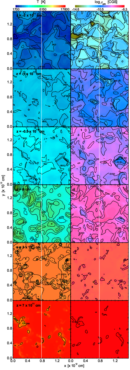
Figure 5: Temperature (left) and density (right) maps in the typical 3D snapshot of the red giant model constructed at different geometrical depth, $z$, with $z=0$ set at $\log\tau_{\rm Ross}=0$ and increasing towards the stellar center. Contours are drawn at every 200 K (panels 1–3, top-down) and 500 K (panels 4–6) for temperature, and 0.5 dex (panels 1–4, top-down) and 0.1 dex (panels 5–6) for density. Vertical lines mark the $x$ position ($x=7.77\times 10^{11}$ cm) at which the 1-dimensional velocity profiles shown in Fig. 9 were constructed.

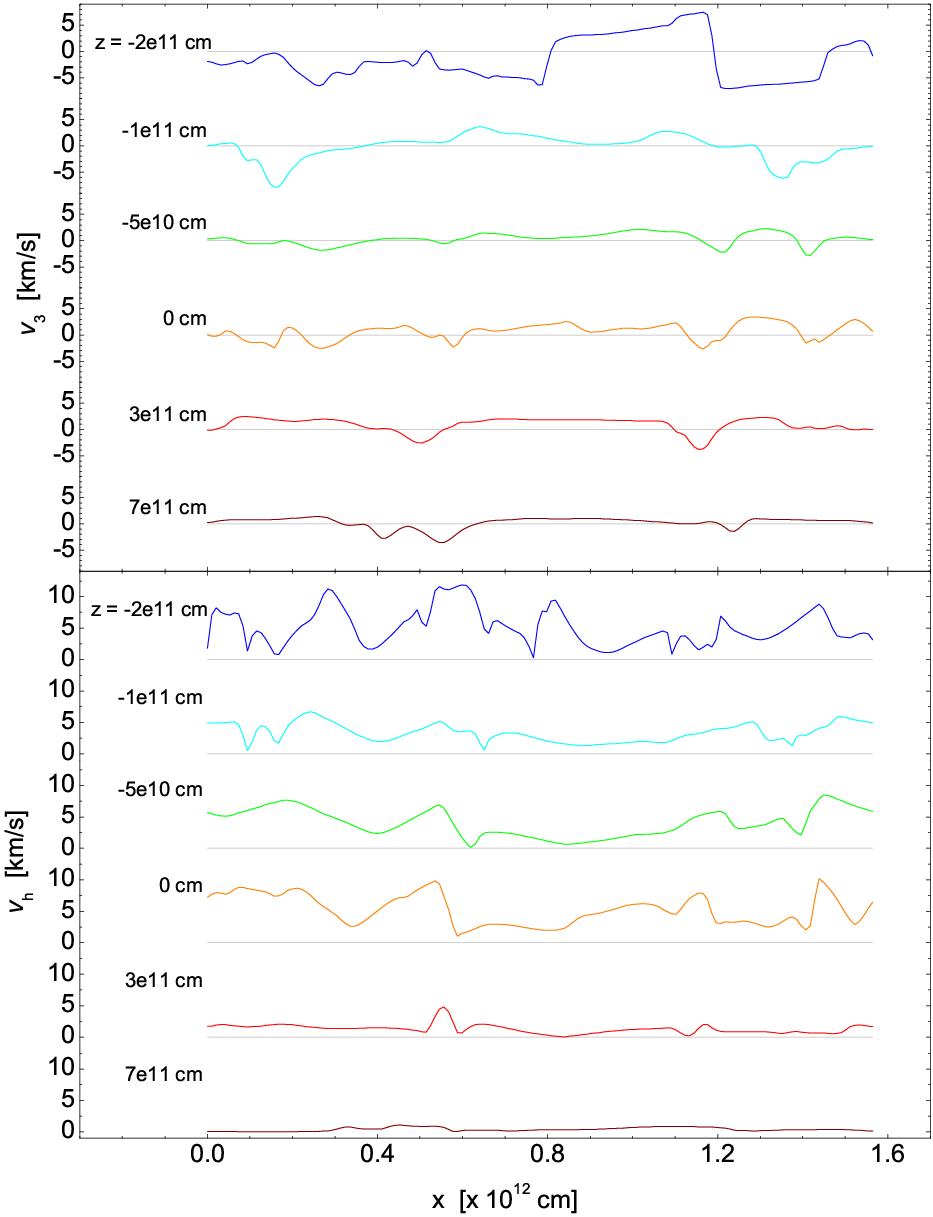
Figure 6: 1-dimensional vertical (top) and horizontal (bottom) velocity profiles in the red giant model at $x=7.77\times 10^{11}$ cm (marked the by white vertical lines in Fig. 4) and shown at different geometrical depths as indicated on the left-hand side of each velocity profile. Grey horizontal lines indicate the level where the velocity is equal to zero.

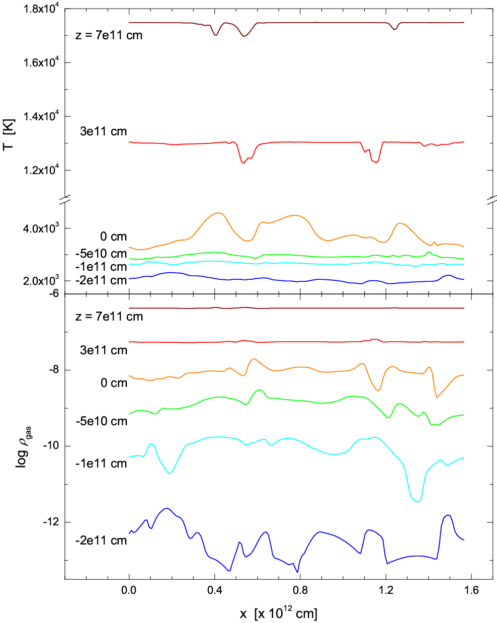
Figure 7: 1-dimensional profiles of temperature (top) and density (bottom) at $x=7.77\times 10^{11}$ cm (marked by the white vertical lines in Fig. 5) and shown at different geometrical depths.

The horizontal flow speed, $v_{\rm h}$, is low in the subphotospheric layers due to the predominantly vertical motions here. The situations starts to change when matter approaches the optical surface. The decreasing opacity leads to enhanced photon losses, the matter rapidly cools, becomes denser, and its vertical velocity decreases. A density inversion is formed just below the optical surface, at $\log\tau_{\rm Ross}\approx 0.5$ (see Fig. 9). Simultaneously, the up-flowing material is deflected sideways until it reaches the granule edges finally merging into the down-flows. The resulting pattern of horizontal velocities is tracing the granular shapes and is visible in the atmospheric layers above the optical surface (Fig. 4).

Figure 6 illustrates that the amplitude of the velocity fluctuations on horizontal planes is highest in the outermost layers, and largely shaped by shock waves. This holds for both the vertical and horizontal velocities. Towards deeper layers, the fluctuations in the vertical velocity become noticeably smaller, fluctuations of the horizontal velocity also decrease but to a lesser degree. As alluded to before, this is a consequence of the take-over of the more regular convective motions over wave motions. After passing a minimum around the optical surface the fluctuations of the vertical velocity increase again, a signature of the roughly columnar flow pattern in the the subphotospheric layers.

As shown in Fig. 7 the columnar pattern in the subphotosphere is also imprinted in the temperature field which is rather homogeneous in the up-flows, and drops in the temperature marking down-flows. The temperature fluctuations reach their maximum in the surface layers, and are quickly reduced in amplitude in the optical thin layers. This is surprising in view of the substantial density fluctuations (see Fig. 7, lower panel) present in the photospheric layers. This indicates an efficient smoothing of the temperature field by radiative energy exchange counteracting temperature changes by adiabatic compression or expansion. The vertical cuts in Fig. 8 and 9 show that the shock waves form a rather irregular pattern in the upper atmosphere. The shock fronts are often horizontal or arc-like, similar to those seen in the 3D hydrodynamical models of the Sun (e.g., Wedemeyer et al., 2004). Most of the shock activity takes place above $z=-0.5\times 10^{11}$ cm ($\log\tau_{\rm Ross}<-1.0$) where the flow density is low enough for the flow to accelerate to supersonic speeds.

Finally, we would like to point out that our model is rather shallow in the sense that its extent below the optical surface supercedes the horizontal size of granular cells only little. Consequently, the merging and narrowing of downdrafts with depth as discussed by Stein & Nordlund (1998) is not clearly discernable. However, qualitative similarity of the convective morphology makes us belief that models with larger extent in depth will exhibit the same feature.

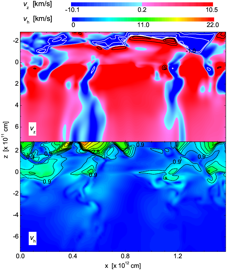
Figure 8: 2D profiles of vertical (top) and horizontal (bottom) velocity in the red giant model at $x=7.77\times 10^{11}$ cm (marked by white vertical lines in Fig. 4). Locations where the vertical velocity $v_{\rm z}\leqslant-1$ Mach (supersonic down-flows, top panel) are marked with white contours, those where $v_{\rm z}$ and $v_{\rm h}$ exceed 1 Mach are contoured in black (contours start at ${\rm Mach}=\pm 1.0$ and are drawn at every $\pm 0.5$ Mach thereof).

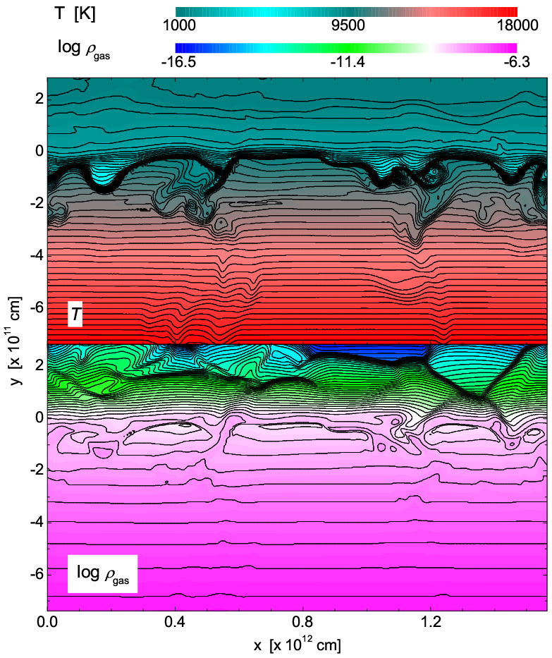
Figure 9: 2D profiles of temperature (top) and density (bottom) in the red giant model at $x=7.77\times 10^{11}$ cm (marked by white vertical lines in Fig. 5). Contours are drawn at every 250 K (top) and 0.2 dex (bottom).

3.2.2 Properties of the $\left\langle\mbox{3D}\right\rangle$ stratification

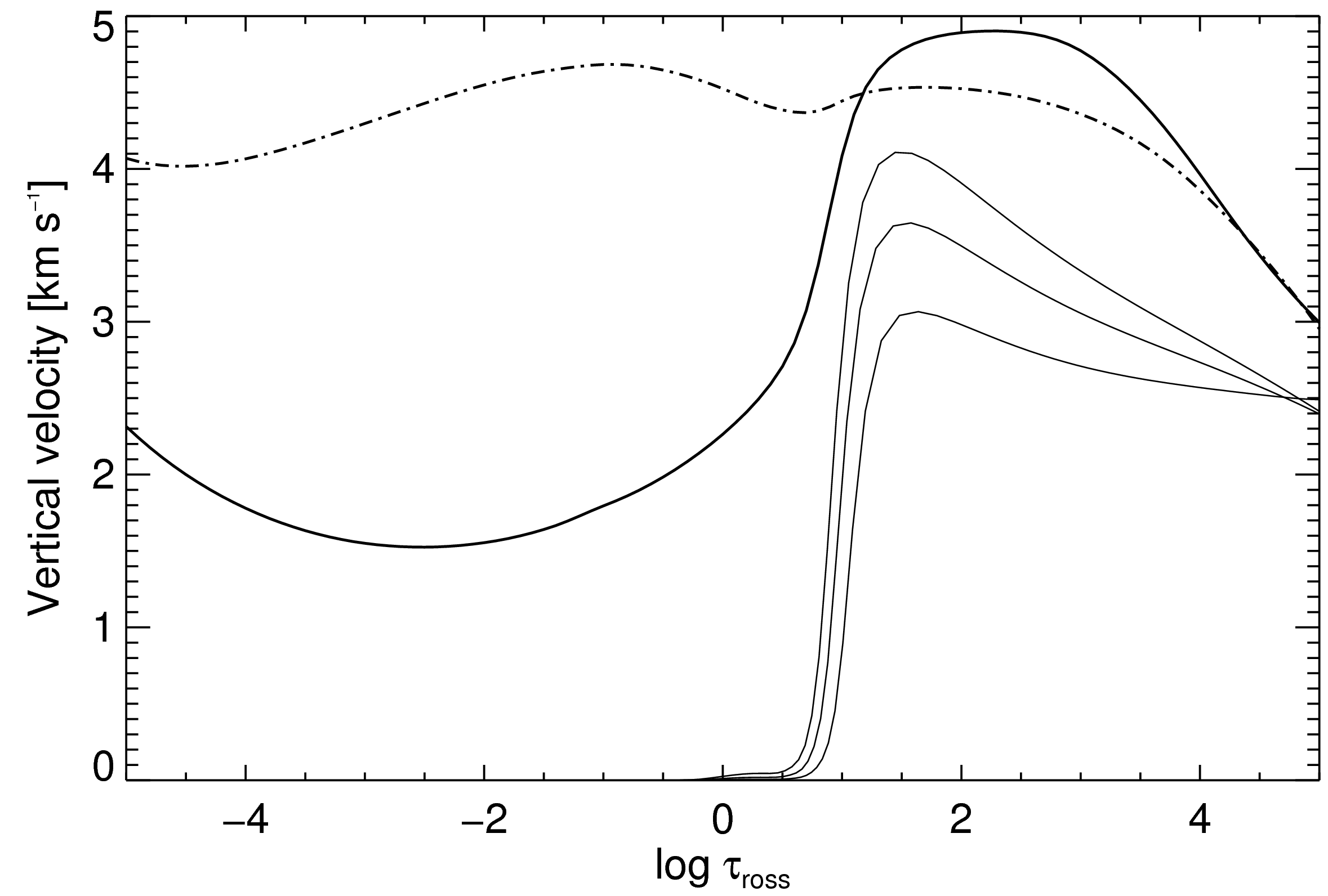
Figure 10: Temporally and horizontally averaged RMS vertical velocity (thick solid line) and RMS horizontal velocity (thick dot-dashed line) of the 3D hydrodynamical model in comparison to the 1D LHD models (thin lines) as a function of Rosseland optical depth. The LHD models were calculated using different mixing-length parameter, $\alpha_{\mathrm{MLT}}=1.0,1.5,2.0$ (top-down).

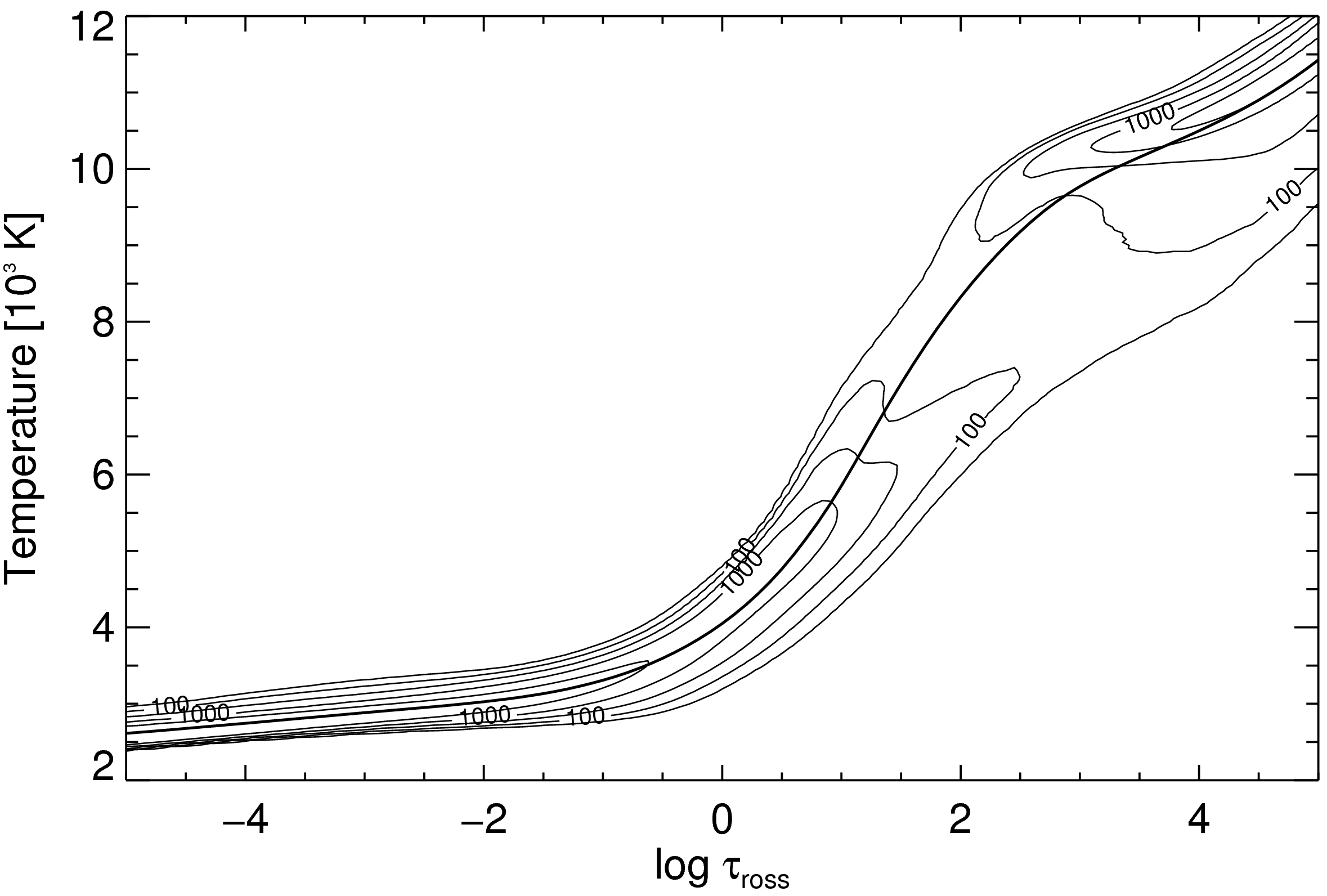
Figure 11: Non-normalized joint probability density function of temperature and optical depth (thin contour lines), and average temperature profile (thick solid line) of the 3D model. The statistics was obtained from three snapshots of the flow field. The contour lines are plotted in steps of factors of $\sqrt{10}$.

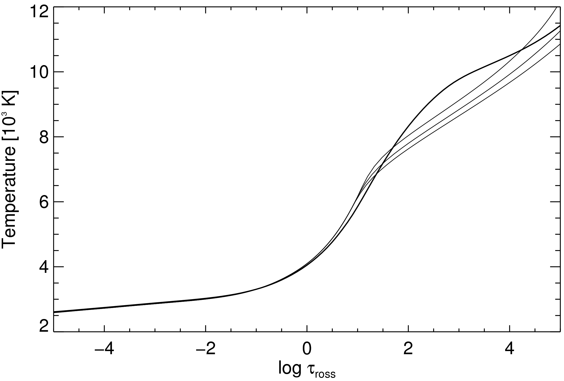
Figure 12: Temperature profile of the $\left\langle\mbox{3D}\right\rangle$ model (thick solid line) in comparison to 1D LHD models (thin solid lines) as a function of Rosseland optical depth. The LHD models were calculated with different mixing-length parameters, $\alpha_{\mathrm{MLT}}=1.0,1.5,2.0$ (upper$\rightarrow$lower).

As we have already seen in Sect. 3.2.1, two regions can be distinguished in the photosphere of the giant model: the lower (and hotter) part dominated by convective motions per se and upper layers where the flow is driven by acoustic waves. This substructure clearly manifests itself in the (temporally and horizontally averaged) RMS vertical and horizontal velocity profiles (Fig. 10). Convective motions gradually cease beyond the formal convective boundary at $\log\tau_{\rm Ross}\sim 0.5$. However, the matter partially penetrates beyond it in a form of exponentially decreasing overshoot. Qualitatively, this is very similar to the picture seen in late-type dwarfs (Ludwig et al., 2002, 2006).

The temperature profile of the $\left\langle\mbox{3D}\right\rangle$ model follows closely the ridgeline corresponding to the maxima of the probability density distribution of temperature and optical depth in the 3D hydrodynamical model (Fig. 11). A sharp decrease both in the 3D and $\left\langle\mbox{3D}\right\rangle$ temperature profiles between the optical depths of $\log\tau_{\rm Ross}=0$ and 2.0 is caused by the rapid increase in the radiative cooling rate close to the optical surface.

Interestingly, the temperature profile corresponding to the $\left\langle\mbox{3D}\right\rangle$ model is markedly different from the 1D temperature profiles in the deeper atmosphere, at $\log\tau_{\rm Ross}>0.5$ (Fig. 12). Moreover, none of the 1D LHD models with different mixing-length parameters, $\alpha_{\rm MLT}$, is able to satisfactorily reproduce the stratification of the $\left\langle\mbox{3D}\right\rangle$ model. The resulting different pressure–temperature relation have a direct influence on the radius of the star. Note, that turbulent pressure was neglected in the 1D LHD models at this stage.

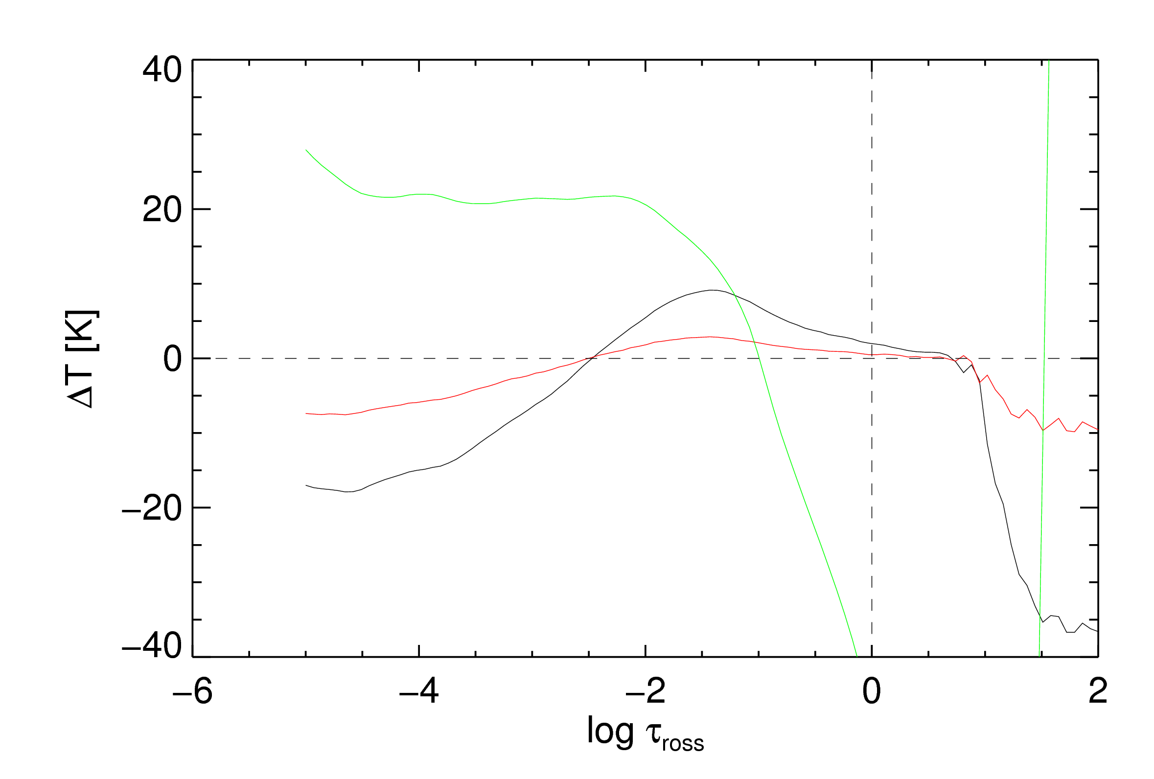
Figure 13: Deviations of temperature profiles from the LHD ($\alpha_{\mathrm{MLT}}$=2.0) convective-radiative equilibrium model. The green line shows the $\left\langle\mbox{3D}\right\rangle$ model, red and black lines depict LHD models with different overshooting velocities, $v_{\mathrm{over}}$=1 km s^-1 and $v_{\mathrm{over}}$=2 km s^-1, respectively.

Figure 13 shows that in the higher atmosphere the 3D model exhibits a temperature increase of about 20 K relative to pure radiative equilibrium conditions. Energy fluxes show that this is not the consequence of mechanical heating (e.g. by shocks). Only the radiative flux provides significant energy exchange in these layers. LHD models with an ad-hoc overshooting velocity show a certain degree of cooling. The cooling is not great despite the substantial overshooting velocities put into the 1D models. This again illustrates the rather tight coupling of the temperature to radiative equilibrium conditions as already seen by the rather small horizontal temperature fluctuations in the upper photosphere. We argue that the heating in the 3D case is due to an altered radiative equilibrium temperature in the presence of horizontal $T$-inhomogeneities and the specific wavelength-dependence of the opacity (see Appendix B). Interestingly, this is opposite to what is seen in the outer atmosphere of red giants at lower metallicities, where the average temperature of the hydrodynamical model is significantly lower than that of the corresponding 1D model (e.g., Collet et al., 2007; Dobrovolskas et al., 2010; Ivanauskas et al., 2010).

3.2.3 Radiative, hydrodynamical and rotational time scales

In order to asses the possible interplay between various physical phenomena that take place in the red giant atmospheres we calculated a number of characteristic radiative and hydrodynamic time scales (see Appendix A for the definitions). The time scales were calculated using the 3D model as background, and are plotted versus the optical depth in Fig. 14.

Two convection-related time scales, as given by the Brunt-Väisälä period, $t_{\rm BV}$, and the time for crossing one mixing-length, $t_{\rm adv}$, are similar within an order of magnitude and show little variation throughout the entire atmosphere. The radiative time scale taking into account the wavelength dependence of the opacity, $t_{\rm rad}$ is significantly larger than convective times scales in the deep atmosphere where the flow is nearly adiabatic. However, $t_{\rm rad}$ rapidly decreases with increasing height and above $\log\tau_{\rm Ross}\sim 2$ becomes about two orders of magnitude shorter than either $t_{\rm BV}$ or $t_{\rm adv}$, thus causing a rapid evolution of the flow towards radiative equilibrium. For further comparison we added the radiative time scale $t_{\rm rad}\mbox{(Ross)}$ based on grey Rosseland opacities. In the optically thin region it substantially overestimates the radiative relaxation time.

The time scale of thermal relaxation, or Kelvin-Helmholtz time scale, $t_{\rm KH}$ is considerably larger than the convective time scale deep in the atmosphere ($\log\tau_{\rm Ross}>4$). This may suggest that the flow in the deeper atmosphere will not be able to relax to thermal equilibrium during the model simulation time, $\sim 6\times 10^{6}$ sec (see Sect. 2), which is $\sim 1-2$ orders of magnitude smaller than $t_{\rm KH}$. However, such conclusion would be wrong, since at these depths thermal relaxation is in fact governed by the mass exchange due to convection which takes place on significantly shorter time scales.

The assessment of whether stellar rotation may influence the dynamical and radiative processes in the atmospheres of red giants is not a trivial task, especially since their rotational periods are largely unknown. In order to obtain a qualitative picture one may nevertheless compare the relevant time scales. To derive an estimate of the rotational time scale we resorted to the available measurements of projected rotational velocities, $v_{\rm rot}\sin i$. For red giants these are are typically in the range of $2-9$ km/s (e.g., Carney et al., 2008; Cortés et al., 2009). Ignoring the fact that rotational velocity, $v_{\rm rot}$, may depend on the effective temperature (Carney et al., 2008) and metallicity (Cortés et al., 2009), and taking $3$ km/s as a representative rotational velocity, together with a radius of $\sim\,75\,{\rm R_{\odot}}$ (see Sect. 2) one obtains the rotation period of $\sim 10^{8}$ sec. This is by at least 1–2 orders of magnitude larger than the convective and radiative time scales, except in the deepest layers where the radiative time scale is longer. While we therefore conclude that rotation should have a minor influence on governing the atmospheric dynamics of this particular red giant, it should be noted that in the deeper atmosphere rotational and convective time scales may become comparable and thus the interaction between convection and rotation interaction may become non-negligible.

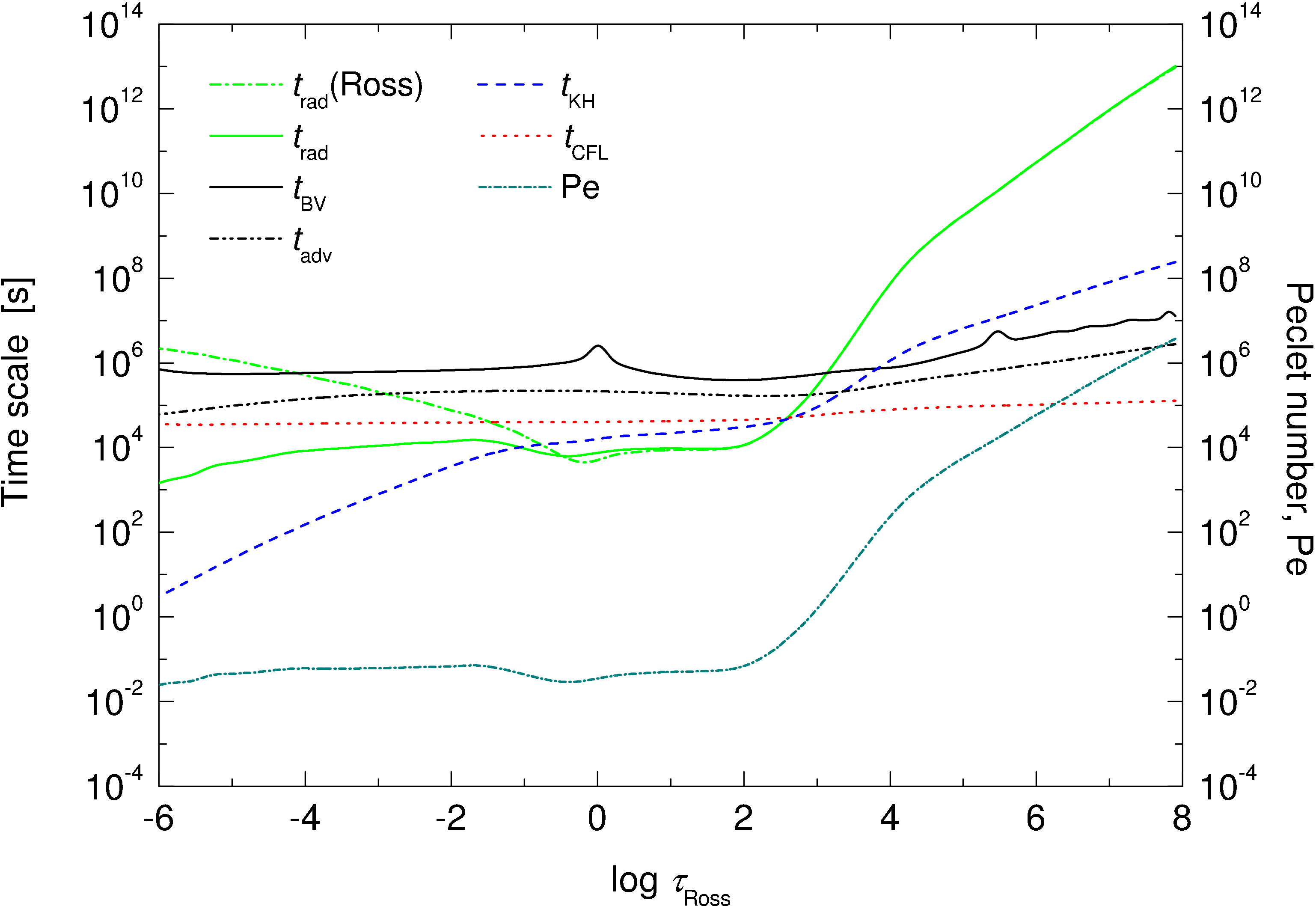
Figure 14: Radiative and hydrodynamical time scales in the 3D atmosphere model of red giant.

3.2.4 The role of turbulent pressure

One of fundamental differences between the 3D hydrodynamical and classical 1D atmosphere models of red giants is that hydrodynamical models predict non-zero turbulent pressure, $P_{\rm turb}$. The contribution of the turbulent pressure to the total pressure (i.e., gas and turbulent) may be as large as $15\%$ in the 3D hydrodynamical models of the Sun (Houdek, 2010). In order to assess its importance in the red giant atmosphere we calculated the turbulent pressure as $P_{\rm turb}=\langle\rho v_{\mathrm{z}}^{2}\rangle$, where $\rho$ and $v_{\mathrm{z}}$ are gas density and velocity, respectively, and angular brackets denote temporal averaging as well as averaging on surfaces of equal optical depth. The ratio of turbulent to total pressure is plotted versus optical depth in Fig. 16.

Although rarely done in the routine calculations of, e.g., 1D stellar model atmosphere grids, in principle turbulent pressure can be included in the calculation of classical 1D atmosphere models, in addition to gas and electron pressure. The result of such an exercise is shown in Fig. 15, where we plot two LHD models calculated with non-zero turbulent pressure ($P_{\rm turb}=f\rho v^{2}$, here $v$ is convective velocity as given in the framework of MLT, and $f$ a dimensionless factor, usually $f<1$). Three additional models shown there were constructed using different mixing-length parameters, $\alpha_{\rm MLT}=1.0,1.5,2.0$, utilizing a formalism of Mihalas (1978) and assuming a vanishing turbulent pressure, $P_{\rm turb}=0$. As it is evident from Fig. 15, there is no reasonable combination of $\alpha_{\rm MLT}$ and $f$ allowing to construct a classical 1D model which would reproduce the pressure–temperature relation of 3D hydrodynamical model.

How important then is the contribution of turbulent pressure in the atmospheres of red giants in general? In the 3D hydrodynamical model atmosphere of a red giant studied here $P_{\rm turb}$ provides a non-vanishing contribution to the total pressure nearly throughout the entire atmosphere, except for the deepest layers where its influence is minor (Fig. 16). The distribution of $P_{\rm turb}/(P_{\rm gas}+P_{\rm turb})$ is double-peaked: the first maximum at $\log\tau_{\rm Ross}\sim 4$ is due to increasing relative importance of convective flow, whereas the monotonous rise beyond $\log\tau_{\rm Ross}\sim-2$ is due to wave activity in the upper atmosphere. The peak values are significantly larger than those in the Sun (cf. Houdek, 2010): the contribution of turbulent pressure may amount to $\sim 25\%$ and $\sim 13\%$ due to convective motions close to the optical surface in the red giant and the Sun, respectively.

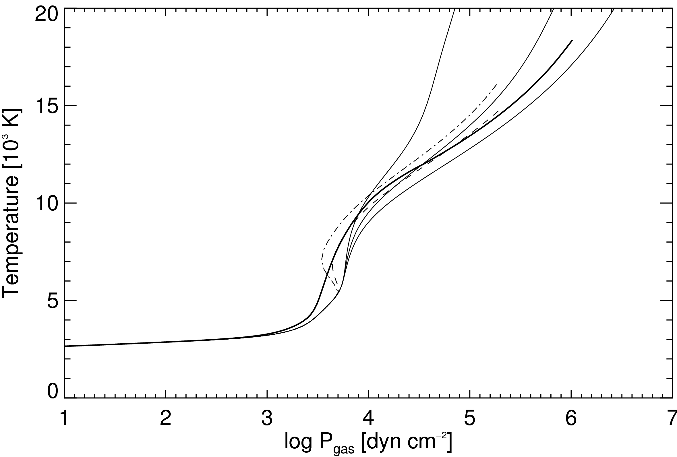
Figure 15: Temperature stratification in the 3D hydrodynamical model of a red giant, as a function of gas pressure, $P_{\rm gas}$. The thick solid line is the profile of the $\left\langle\mbox{3D}\right\rangle$ model, the thin lines are 1D LHD models calculated using different mixing-length parameter ($\alpha_{\rm MLT}=1.0,1.5,2.0$, from left to right; in all cases $P_{\rm turb}=0$). The two 1D models with non-zero turbulent pressure are shown by dashed ($\alpha_{\rm MLT}=2.0$ and $f=1.0$) and dashed-dotted ($\alpha_{\rm MLT}=2.0$ and $f=2.0$) lines.

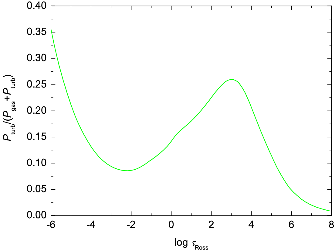
Figure 16: Turbulent pressure to total pressure versus optical depth in the 3D model.

Obviously, the importance of turbulent pressure can not be neglected in realistic modeling of stellar atmospheres and stellar evolution. One may argue that in the case of the red giant studied here the discrepancy between the pressure–temperature relations of the 3D hydrodynamical and 1D models occurs deep in the atmosphere ($\log\tau_{\rm Ross}\sim 2$) and thus should have a minor influence on the formation of emitted spectrum. However, this may be of importance for giants at lower metallicities where convection can reach into the layers beyond the optical surface. Additionally, larger pressure at any given geometrical depth would lift the higher-lying stellar layers outwards and may eventually change the stellar radius and luminosity, with direct consequences on the evolutionary tracks and isochrones. Clearly, issues related with the proper treatment of turbulent pressure in the current stellar evolution and atmosphere modeling of red giants warrant further study.

3.2.5 Effective mixing-length parameter for the 1D model atmospheres

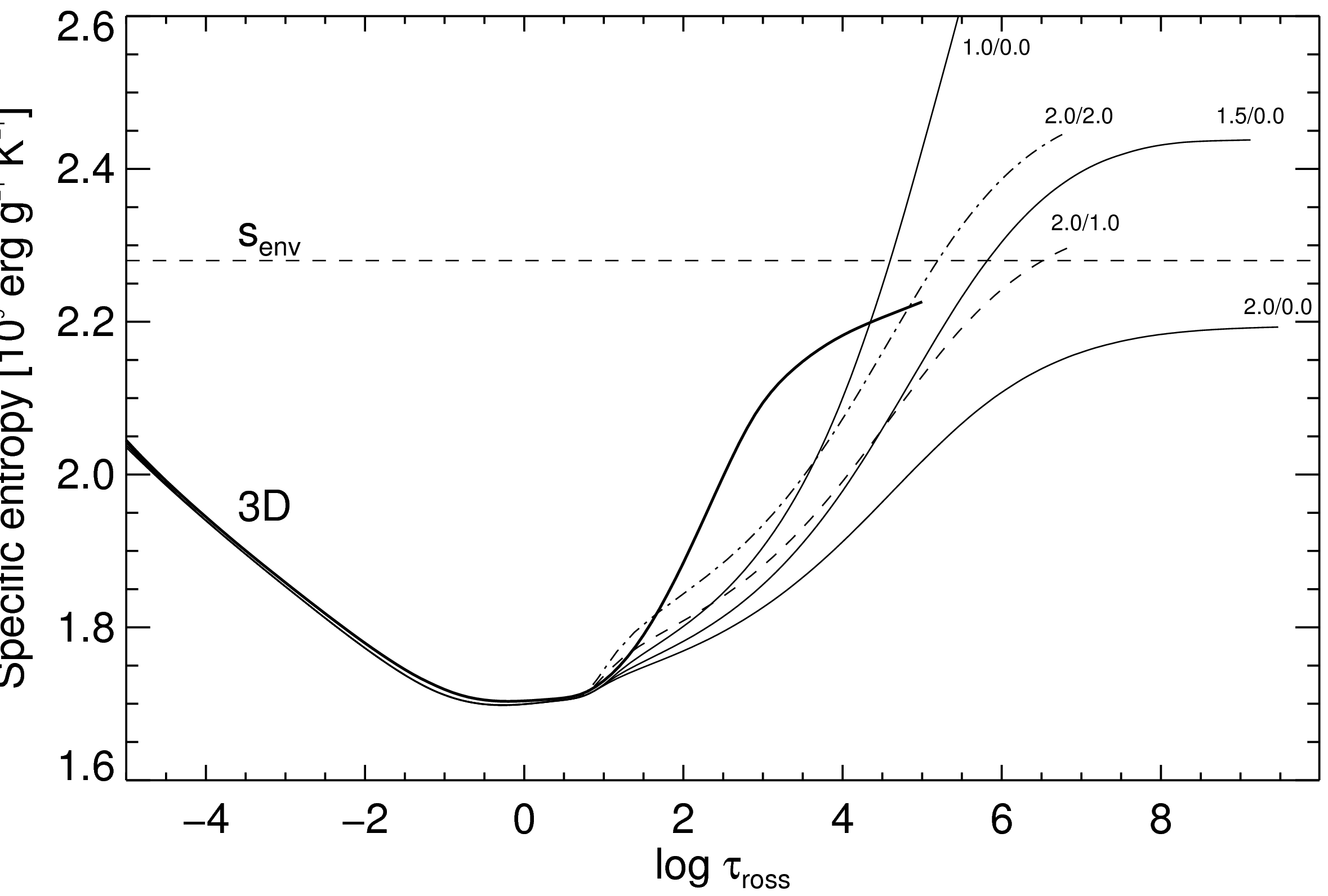
Figure 17: Entropy profiles as a function of optical depth. The dashed line indicates the value of the asymptotically reached entropy in the 3D model. Thick solid line is entropy stratification of the temporally and spatially averaged $\left\langle\mbox{3D}\right\rangle$ model, thin lines are 1D LHD models calculated with different mixing-length parameters, $\alpha_{\mathrm{MLT}}=1.0,1.5,2.0$ (left-to-right). The two models with non-zero turbulent pressure are shown by dashed ($\alpha_{\mathrm{MLT}}=2.0$ and $f=1.0$) and dash-dotted ($\alpha_{\mathrm{MLT}}=2.0$ and $f=2.0$) lines.

The potential of the hydrodynamical model atmospheres for the calibration of the mixing-length parameter, $\alpha_{\mathrm{MLT}}$, was explored by Ludwig et al. (1999). The authors have shown that the entropy profiles in the 2D models of solar-type stars posses a minimum in the convectively unstable region. While the shape and location of this entropy minimum is somewhat different in individual spatially resolved profiles, the common property is that the entropy gradient becomes very small in the deep atmospheric layers where the adiabatic up-flows dominate. Such asymptotic behavior is also characteristic to 1D model atmospheres but the asymptotic entropy values reached deep in the atmosphere are different for different mixing-length parameters, $\alpha_{\mathrm{MLT}}$. Therefore, the height of the asymptotic entropy plateau in the 2D hydrodynamical models can be used to calibrate the $\alpha_{\mathrm{MLT}}$ for use with 1D models (Ludwig et al., 1999). Further steps in this direction were made by Ludwig et al. (2002) who demonstrated that this approach works well also with the 3D hydrodynamical model of M-type dwarf.

In order to check the feasibility of such approach with the red giant model studied here, we utilized the set of LHD models calculated in the previous section using different values of $\alpha_{\mathrm{MLT}}$ and plotted their entropy profiles versus the optical depth in Fig. 17. Also shown there are the temporally and spatially averaged specific entropy profiles of the $\left\langle\mbox{3D}\right\rangle$ model. Clearly, the 3D entropy profile shows hints of an asymptotic flattening, similarly to what is seen in the 1D models. We emphasize that horizontally resolved entropy profiles show a plateau at a value indicated by $s_{\mathrm{env}}$ in Fig. 17. Interpolation between the asymptotic entropy values found in the 1D models with different values of the mixing-length parameter and zero turbulent pressure yields $\alpha_{\mathrm{MLT}}\sim 1.8$.

One remark of caution is here again related to the turbulent pressure. Evidently, one may get significantly different $\alpha_{\mathrm{MLT}}$ values for the 1D models characterized by different turbulent pressure, $P_{\rm turb}$ (Fig. 17). As we have seen in the previous section, there is no straightforward procedure to calibrate turbulent pressure with the aid of $\left\langle\mbox{3D}\right\rangle$ models. Moreover, the net effect of the individual spatially resolved entropy profiles will be always different from that given by the $\left\langle\mbox{3D}\right\rangle$ model. These facts once again stress the importance and difficulties of the proper incorporation of turbulent pressure into the atmospheric and evolutionary models of red giants.

3.2.6 How realistic is our 3D hydrodynamical model?

Obviously, the realism of the 3D hydrodynamical model discussed in this study is limited by a number of the assumptions used in the modeling procedure. Some issues need to be mentioned here.

Our model of a red giant has limited grid resolution of $150\times 150$ horizontal grid points spread over $\sim 1/6\times 1/6$ of the stellar surface. While such coverage and resolution may be sufficient to pin down the general properties of atmospheric stratifications, substantially better resolution would be needed to investigate the properties of atmospheric motions on smaller scales. Moreover, the fraction of the surface area covered by the model is already large and so the effects of sphericity may become important. These issues should be addressed in future work.

As was described in Sect. 2.1, we used monochromatic opacities grouped into 5 opacity bins to reduce the computational work load. Previous studies and tests that we did in the course of the present study have demonstrated that opacity grouping yields a surprisingly good agreement with the exact radiative transfer calculations obtained using opacity distribution functions, ODFs (see, e.g., Nordlund, 1982; Collet et al., 2007). One has to be cautious, however, since the effects related to molecular opacities may become increasingly important in the outer atmospheres of red giants, and the opacity grouping into small number of bins may be insufficient.

One more issue of concern may be related with the treatment of scattering. It has been shown by Collet et al. (2007, 2008) that scattering treated as true absorption may produce significantly warmer temperature profiles in the outer atmospheres of red giants at low metallicities, compared to those that are obtained when scattering is treated properly. The treatment of coherent and isotropic scattering in the solution of radiative transfer equation was recently implemented in the 3D hydrodynamical code BIFROST by Hayek et al. (2010). While it seems that in general the continuum scattering does not have large effect on the thermal structure in the atmospheric model of the Sun, proper inclusion of scattering in the line blanketing may reduce the temperature by $\sim 350$ K in the optically thin layers below $\log\tau_{\rm 5000}\lesssim-4$ (Hayek et al., 2010). Obviously, this issue has to be addressed properly in the future 3D hydrodynamical modeling of red giants, however, is mainly an issue for metal-poor objects.

4 Conclusions and outlook

In this study we have utilized a 3D hydrodynamical model of a red giant calculated with the CO⁵BOLD code to investigate the influence of convection on the properties of its atmospheric structures. The model had solar metallicity and its atmospheric parameters, $T_{\rm eff}=3660$ K and $\log g=1.0$, were typical to those of a red giant located close to the RGB tip. We also used a number of 1D atmosphere models calculated with the LHD code to compare the predictions of the 3D hydrodynamical model with those of classical 1D models. The 1D LHD model atmospheres shared the same opacities and equation-of-state as used in the calculations of the 3D hydrodynamical models and covered the same range in the optical depth. Thus, the comparison was done in a strictly differential way, to ensure that the differences revealed would reflect solely the differences related to dimensionality between the two types of models.

Similarly to what is seen in dwarfs, the giant model predicts the existence of pronounced surface granulation pattern with a white light intensity contrast larger than in solar models ($\sim 18\%$ versus $\sim 15\%$, respectively). The size of the granules relative to the available stellar surface is significantly larger in the giant than in the Sun, with a typical ratio of $\sim 400$ and $\sim 2\times 10^{6}$ granules over surface area, respectively. This, together with the larger intensity (and temperature) contrast in the giant model suggests that convection may have substantially larger influence on the observable properties (such as spectral energy distribution, photometric colors) of red giants than in the Sun. Exploratory work in this direction seems to confirm this prediction (Kučinskas et al., 2009, 2010).

It is important to note that the atmosphere model displays a significant activity of shock waves, especially in the outer atmosphere. In comparison with the mild shocks in models of the Sun, with vertical and horizontal velocities of up to Mach $\sim 1.5$ and $\sim 1.8$, respectively, the shocks in the atmosphere of the giant are considerably stronger, with corresponding Mach numbers of $\sim 2.5$ and $\sim 6$. We also find that the mean temperature of the hydrodynamical model is slightly higher than that of the 1D model with identical atmospheric parameters.

Turbulent pressure is considerably more important in the giant model than it is in the Sun and may amount to $\sim 35\%$ of the total pressure (i.e., gas plus turbulent). This leads to a lifting of the outer atmospheric layers to larger radii, besides, it would alter the pressure-temperature relation. Interestingly, no combination of the mixing-length parameter and turbulent pressure in the 1D models satisfactorily reproduce the mean pressure-temperature relation of the hydrodynamical model.

We used the 3D hydrodynamical model to obtain the effective mixing-length parameter for the classical 1D stellar atmosphere work. Interpolation between the entropy profiles of the 1D models calculated with different mixing-length parameters and zero turbulent pressure yields $\alpha_{\mathrm{MLT}}=1.8$. This solution, however, is not unique since identical mixing-length parameter may be obtained for models characterized by different amount of turbulent pressure. The question of how to treat the turbulent pressure in the 1D models of stellar atmospheres and stellar evolution, therefore, still remains open. In view of Fig. 15 it appears unlikely that this can be addressed within the framework of MLT when assuming a sharp boundary of the convectively unstable region. In one way or another some “softening” by overshooting needs to be introduced. 3D models can give some quantitative guidance here. The indirect feedback of horizontal inhomogeneities on the vertical structure is also included in this way.

Obviously, the 3D hydrodynamical stellar atmosphere model studied in this work is rather an exploratory one. There is still some way to go for improving the 3D models so that they could match the realism of the current 1D stationary stellar model atmospheres in the treatment of opacities, equation-of-state, radiative transfer, and scattering. We believe, nevertheless, that the advantages of the 3D hydrodynamical models over their classical 1D counterparts are obvious, which warrants further efforts towards their firmer implementation in the field of stellar atmosphere studies.

Appendix A Computation of the characteristic time scales

The time scales in the red giant explored in this work (see Sect. 3.2.3) were calculated following the prescriptions given in Ludwig et al. (2002, 2006).

The radiative relaxation time, $t_{\mathrm{rad}}$, can be evaluated using the MLT formula

$$t_{\mathrm{rad}}=\frac{\rho c_{\mathrm{p}}\Lambda\tau_{\mathrm{e}}}{f_{3}\sigma T^{3}}\,\left(1+\frac{f_{4}}{\tau_{\mathrm{e}}^{2}}\right),$$ (1)

where $\rho$ is gas density, $c_{\mathrm{p}}$ the specific heat at constant pressure, $\Lambda=\alpha_{\mathrm{MLT}}H_{\mathrm{P}}$ the mixing-length, $\sigma$ Stefan-Boltzmann constant, $T$ gas temperature, $f_{3}=16$ and $f_{4}=2$ dimensionless constants in the MLT formulation of Mihalas (see Ludwig et al. 1999). The optical thickness of a convective element, $\tau_{e}$, is defined as $\tau_{\mathrm{e}}\equiv\chi\rho\Lambda$, where $\chi$ is opacity.

It can be shown that in the case of non-grey radiative transfer with opacities grouped into $i$ opacity bins, Eq. (1) can be re-written as

$$t_{\mathrm{rad}}=\frac{\rho c_{\mathrm{p}}\Lambda}{f_{3}\sigma T^{3}}\,\left(\sum_{i}w_{\rm i}\frac{\tau_{\rm i}}{f_{4}+\tau_{\rm i}^{2}}\right)^{-1},$$ (2)

where the optical thickness of convective element is now different in each opacity bin

$$\tau_{\rm i}\equiv\chi_{\rm i}\rho\Lambda$$ (3)

and $\chi_{\rm i}$ is opacity in bin $i$. Eq. (2) was used to estimate the radiative time scale in the atmosphere of a red giant model studied here, with the weights $w_{\rm i}$ for the different opacity bins evaluated using

$$w_{\rm i}=b_{\rm i}+\frac{T}{4}\frac{db_{\rm i}}{dT}$$ (4)

where $b_{\rm i}=B_{\rm i}/B$ and $B=\frac{\sigma}{\pi}T^{4}$. The mixing-length parameter used in the calculations was set to $\alpha_{\mathrm{MLT}}$=1.8, in accordance with the value derived in Sect. 3.2.5.

The advection time scale, $t_{\mathrm{adv}}$, was estimated as time interval during which the convective element travels one mixing-length

$$t_{\mathrm{adv}}=\frac{\Lambda}{v_{\mathrm{z}}^{\mathrm{rms}}},$$ (5)

where $v_{\mathrm{z}}^{\mathrm{rms}}$ is temporally and horizontally averaged vertical RMS velocity.

The adiabatic Brunnt-Väisälä period, $t_{\mathrm{BV}}$, was obtained using

$$t_{\mathrm{BV}}=\frac{2\pi}{\sqrt{|\omega_{\mathrm{BV}}^{2}|}},$$ (6)

with

$$\omega_{\mathrm{BV}}^{2}=\frac{\delta g}{H_{\mathrm{P}}}(\nabla_{\mathrm{ad}}-\nabla).$$ (7)

where $\delta\equiv-(\frac{\partial\rho}{\partial T})_{\mathrm{P}}$ is the thermal expansion coefficient at constant pressure, $g$ gravitational acceleration, $\nabla_{\mathrm{ad}}$ and $\nabla$ the adiabatic and actual temperature gradients, respectively.

The Kelvin-Helmholtz time scale, $t_{\mathrm{KH}}$, was calculated using

$$t_{\mathrm{KH}}=\frac{Pc_{\mathrm{p}}T}{g\sigma T_{\mathrm{eff}}^{4}},$$ (8)

where $P$ is gas pressure.

Finally, the relative importance of radiative and advective heat transport was estimated using the Péclet number

$${\rm Pe}\equiv\frac{t_{\mathrm{rad}}}{t_{\mathrm{adv}}}.$$ (9)

Appendix B Changes of the radiative equilibrium temperature due to spatial brightness fluctuations

In Sect. 3.2.2 we found a slight ($\sim 20$ K) increase of the mean atmospheric temperature of the 3D model in the upper atmosphere relative to the radiative equilibrium temperature of a plane-parallel 1D model atmosphere. 3D and 1D model share the same effective temperature (and gravity). We want to demonstrate here that this temperature increase in the 3D model can be interpreted as a change of the radiative equilibrium temperature caused by the spatial fluctuations of the brightness in deeper atmospheric layers due to the convection pattern present in the 3D model. To this end, we develop a simple model describing the establishment of the radiative equilibrium temperature when brightness fluctuations are present.

The radiative equilibrium temperature is established by the balance of absorbed radiation coming from deeper layers and the radiation emitted according to the local temperature. We consider the radiation field as simply given by the Kirchhoff-Planck function $B_{\lambda}(T)$ of radiation temperature $T$. In the plane-parallel case the balance between emission at local temperature $T_{1}$ and absorption of radiation coming from the deeper atmospheric layers with radiation temperature $T_{0}$ can be written as

$$\int\!d\lambda\,\kappa_{\lambda}(T_{1})B_{\lambda}(T_{1})=f_{\Omega}\int\!d\lambda\,\kappa_{\lambda}(T_{1})B_{\lambda}(T_{0})$$ (10)

where $\kappa_{\lambda}$ is the opacity and $f_{\Omega}$ the solid angle subtended by the radiating deeper layers. We envision this to be the “stellar surface”, and $T_{0}$ is close to the effective temperature. For brevity, we did not explicitely note the pressure dependence of the opacity $\kappa_{\lambda}(P_{1},T_{1})$ in the above equation. All wavelength integrals in this section should be taken from zero to infinity. $f_{\Omega}$ is $\frac{1}{2}$ in the case of no limb-darkening, decreasing to smaller values as $f_{\Omega}=\frac{1}{2}(1-\frac{1}{2}a)$ for a limb-darkening being described by a linear limb-darkening law with coefficient $a$. We now introduce brightness fluctuations by considering a two component model for the granulation having equal surface area fractions and radiation temperatures $T_{0}+\Delta T_{0}$ and $T_{0}-\Delta T_{0}$. The total emitted flux should correspond to the unperturbed situation so that we have to fulfill the normalization condition

$$f_{B}\int\!d\lambda\,\frac{1}{2}\left\{B_{\lambda}(T_{0}+\Delta T_{0})+B_{\lambda}(T_{0}-\Delta T_{0})\right\}=\int\!d\lambda\,B_{\lambda}(T_{0}),$$ (11)

introducing the normalization factor $f_{B}$. The temperature fluctuations lead to a “hardening” of the radiation field, i.e., a shift of the flux towards the blue part of the spectrum. Since $\int\!d\lambda\,B_{\lambda}(T)=\frac{\sigma}{\pi}T^{4}$ ($\sigma$ indicates Stefan-Boltzmann’s constant), Eq. (11) could be solved exactly for $\Delta T_{0}$. However, here we are content with an approximate – and much simpler – solution for the case $\Delta T_{0}\ll T_{0}$ and obtain to leading order

$$f_{B}\approx\frac{1}{1+6\left(\frac{\Delta T_{0}}{T_{0}}\right)^{2}}.$$ (12)

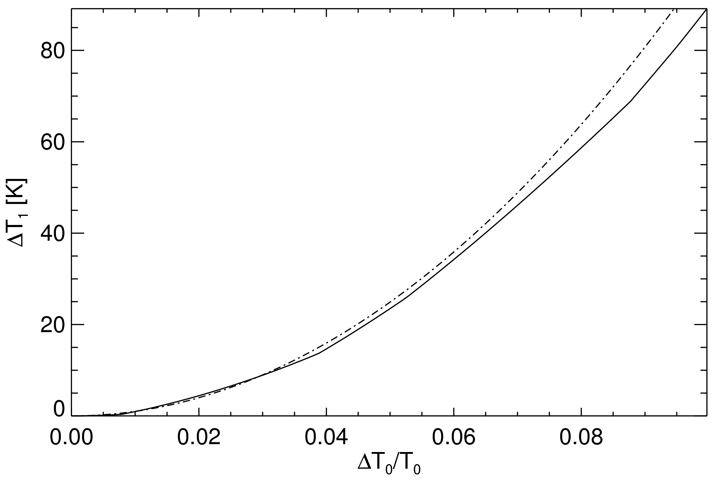
Figure 18: Solid line: change of the radiative equilibrium temperature $\Delta T_{1}$ due to horizontal temperature fluctuations according Eqs. (11) and (13). Dash-dotted line: dependence as given by the linearized solution (14). Further details see text.

We now evaluate the change in the radiative equilibrium temperature $\Delta T_{1}$ relative to the plane-parallel situation due to brightness fluctuations associated with temperature changes of size $\Delta T_{0}$. We use the ansatz (10) to obtain for the relation between emission and absorption at a location in the optically thin layers of the atmosphere

$$\int\!d\lambda\,\kappa_{\lambda}B_{\lambda}(T_{1}+\Delta T_{1})=f_{B}f_{\Omega}\int\!d\lambda\,\kappa_{\lambda}\frac{1}{2}\left\{B_{\lambda}(T_{0}+\Delta T_{0})+B_{\lambda}(T_{0}-\Delta T_{0})\right\}.$$ (13)

Expanding for $\Delta T_{1}\ll T_{1}$ results to leading order in

$$\Delta T_{1}\approx 6f_{\Omega}\left(\frac{\Delta T_{0}}{T_{0}}\right)^{2}\frac{\int\!d\lambda\,\,\kappa_{\lambda}(T_{1})\left[\frac{1}{12}\left.\frac{d^{2}B_{\lambda}}{dT^{2}}\right|_{T_{0}}T_{0}^{2}-B_{\lambda}(T_{0})\right]}{\int\!d\lambda\,\,\kappa_{\lambda}(T_{1})\left.\frac{dB_{\lambda}}{dT}\right|_{T_{1}}}.$$ (14)

Equation (14) shows that the influence of horizontal inhomogeneities on the radiative equilibrium temperature is small since $\Delta T_{1}$ goes as the square of the temperature fluctuations. Moreover, $\Delta T_{1}$ is controlled by the complex dependence of the opacity $\kappa_{\lambda}$ on wavelength: $\Delta T_{1}$ vanishes if the opacity is wavelength-independent. To account for the wavelength dependence of the opacity the integrals in Eq. (14) have to be evaluated numerically. In doing so, we decided to go one step back and evaluate the fundamental equations (11) and (13) before expanding for small $\Delta T_{0}$ and $\Delta T_{1}$. Moreover, we used the binned opacities as applied in the radiative transfer of the 3D and 1D model to approximate the integrals improving consistency of our approximate analytical model with the detailed models. A solution for $\Delta T_{1}$ for given $\Delta T_{0}$ can be found iteratively. For completeness, we also calculated the dependence according Eq. (14), again, evaluating the integrals using the binned opacities.

Figure 18 depicts the result for $T_{0}=3660\,\mbox{K}$, $T_{1}=2900\,\mbox{K}$, and $P_{1}=100\,\mbox{dyn cm}^{-2}$. $T_{0}$ corresponds to the effective temperature of the detailed numerical models, $T_{1}$ and $P_{1}$ to the conditions prevailing around optical depth $\log\tau_{\rm Ross}\sim-3$. $T_{1}$ was adjusted by setting the solid angle fraction to $f_{\Omega}=0.28$ (indicating a rather strong limb-darkening which is actually present). The model indeed predicts a heating of the outer atmosphere while a cooling would be also possible depending on the wavelength-dependence of the opacity. A white light intensity contrast of about 18 % as suggested by Fig. 3 corresponds to a temperature fluctuation of 4.5 %. At this level of fluctuations our simple analytical model predicts an increase of the radiative equilibrium temperature in the optically thin layers close to the $\sim$20 K found in the 3D model (see Fig. 13). Hence, we consider it plausible that the the temperature increase in the optically thin layers in the 3D model relative to 1D plane-parallel models is a consequence of horizontal brightness fluctuations associated with granulation.