Time evolution of autocorrelation function in dynamical replica theory

Abstract

Asynchronous dynamics given by the master equation in the Sherrington–Kirkpatrick (SK) spin-glass model is studied based on dynamical replica theory (DRT) with an extension to take into account the autocorrelation function. The dynamical behaviour of the system is approximately described by dynamical equations of the macroscopic quantities: magnetization, energy contributed by randomness, and the autocorrelation function. The dynamical equations under the replica symmetry assumption are derived by introducing the subshell equipartitioning assumption and exploiting the replica method. The obtained dynamical equations are compared with Monte Carlo (MC) simulations, and it is demonstrated that the proposed formula describes well the time evolution of the autocorrelation function in some parameter regions. The study offers a reasonable description of the autocorrelation function in the SK spin-glass system.

1 Introduction

Random systems that possess frustration have many metastable states in their free energy landscape, which are expected to contribute to the system behaviour. Spin-glass systems are representative of such systems and their equilibrium properties have been extensively studied in a mean-field model, the Sherrington–Kirkpatrick (SK) model. Mean-field theory based on the replica method reveals the existence of a transition associated with replica symmetry breaking (RSB) that is interpreted with the aid of Thouless–Anderson–Palmer (TAP) theory as the exponential appearance of metastable states in the free energy landscape [1, 2]. A quantitative understanding of the metastable states is attempted by counting the number of solutions of the TAP equation or belief propagation equation [3, 4, 5].

Below a critical temperature, spin glasses in experiments show slow relaxation dynamics and an aging effect in which the dynamical properties depend on the history even after a long time period [6]. The dynamical behaviour and equilibrium properties are considered to be related, but the connection is not fully understood. It has been suggested that dynamical behaviour of the SK model is qualitatively similar to spin glasses in experiments even though the realistic spin glasses have finite dimensions [7]. Therefore, clarifying the relaxation dynamics in the SK model provides insight into the connection between the equilibrium and dynamical properties, as well as into the dynamics of random systems. For this purpose, an analytical description of the relaxation dynamics in the SK model that can be compared with our knowledge of the equilibrium states would be of significant use.

Dynamical replica theory (DRT) provides a statistical-mechanical description of the dynamics in random systems [8]. In DRT, the time evolution of macroscopic quantities is derived according to the replica method. A characteristic feature of DRT is the introduction of an assumption called subshell equipartitioning in which the microscopic states in the subshell that are characterized by a certain macroscopic quantity value appear with the same probability. By introducing this assumption, one can obtain closed dynamical equations that describe the time evolution of the macroscopic quantities. The derivation of the dynamical equations and their DRT solutions are tractable even if the relaxation dynamics over long time are considered, although an exact description of the dynamics is sacrificed. DRT offers a contrasting perspective compared to the generating functional method [9, 10] in which the dynamical equations are exact but difficult to solve over long time steps.

The physical implications of subshell equipartitioning and its influence on the accuracy of the theoretical prediction have been studied [11, 12]. The assumption removes the microscopic time correlation, and the system only depends on the past value of the macroscopic quantities that characterize the subshell. It is well known that the time correlation is significant in describing the dynamics of random systems. In fact, it has been demonstrated that analytical descriptions of the dynamics are improved by taking into account the time correlation in the Hopfield model [13, 14] and in the interference canceller of code-division-multiple-access (CDMA) multiuser detection [15]. However, DRT in its present formalism cannot deal with the time correlation, and hence to apply DRT to random systems and discuss the time correlation, an extension should be introduced.

A central quantity in the study of the dynamics of spin glasses is the spin autocorrelation function that describes the correlation between microscopic states at two time steps. It is experimentally and numerically observed with the conjugate response function as a quantity that indicates the slow relaxation dynamics [6] and its analytical description has been studied in particular Langevin dynamics of soft spins [16, 17]. In this paper, I study the sequential dynamics of the SK model with DRT while including the time evolution of the autocorrelation function. DRT has been studied mainly for two cases where the subshell is characterized by a magnetization and energy set contributed by randomness [8] or a conditional local field distribution [18]. I start with the simplest DRT [8] and introduce the autocorrelation function into the formulation. The evolution equation of the autocorrelation function is derived based on the replica method and its dependence on the phase is discussed.

This paper is organized as follows. In section 2, I explain the model settings and time evolution of the joint probability of microscopic states at two time steps, which is described by Glauber dynamics [19]. In section 3, macroscopic quantities, magnetization, energy contributed by randomness, and the autocorrelation function, are introduced to characterize the microscopic state space. The closed formula of the evolutional dynamics of the quantities is obtained following the procedures of DRT, and the expressions under the replica symmetry (RS) assumption are derived. In section 4, the obtained dynamical equations are numerically solved and the results are compared with MC simulations. Finally, section 5 is devoted to conclusions and the outlook for further developments.

2 Model setup

The system being studied here is a mean-field spin-glass model, the SK model, which consists of $N$ Ising spins $\bm{S}=\{S_{i}\}~{}(i=1,\cdots,N)$. The Hamiltonian is given by

$$H(\bm{S}|\bm{J})=-\sum_{i<j}J_{ij}S_{i}S_{j}-h\sum_{i}S_{i},$$ (1)

where $J_{ij}$ is the interaction between spins $S_{i}$ and $S_{j}$, and $h$ is the external field. The interactions $\bm{J}=\{J_{ij}\}$ are symmetric ($J_{ij}=J_{ji}$) and assumed to be independently and identically distributed according to the Gauss distribution with a mean of $J_{0}/N$ and a variance of $J^{2}/N$;

$$P_{J}(J_{ij})=\sqrt{\frac{N}{2\pi J^{2}}}\exp\Big{[}-\frac{N}{2J^{2}}\Big{(}J_{ij}-\frac{J_{0}}{N}\Big{)}^{2}\Big{]}.~{}~{}~{}(i\neq j)$$ (2)

Here, I consider the conditional probability of a microscopic spin configuration $\bm{\sigma}$ at $t_{w}+t$ under a given spin configuration $\bm{s}$ at time $t_{w}$ and interaction $\bm{J}$ as $p(\bm{\sigma};t_{w}+t|\bm{s};t_{w},\bm{J})$. The time $t_{w}$ is called the waiting time. The two configurations $\bm{\sigma}$ and $\bm{s}$ are related to each other through $\bm{\sigma}=\bm{s}\circ\bm{d}$, where $\bm{d}=\{d_{i}\}~{}(i=1,\cdots,N)$ is a vector consisting of Ising variables, and $\circ$ denotes the Hadamard product, which is a product with respect to each component; the $i$-th component of $\bm{s}\circ\bm{d}$ is $s_{i}d_{i}$. When $d_{i}=1$, the $i$-th spin configuration at time $t_{w}$ and that at time $t_{w}+t$ are the same; otherwise they differ. The time evolution of the microscopic conditional probability in the direction of $t$ is given by Glauber dynamics, which is an asynchronous update of spin configurations described by the master equation,

$$\frac{d}{dt}p(\bm{s}\circ\bm{d};t_{w}+t|\bm{s};t_{w},\bm{J}) =\sum_{k=1}^{N}\{p(\bm{s}\circ F_{k}\bm{d};t_{w}+t|\bm{s};t_{w},\bm{J})w_{k}(\bm{s}\circ F_{k}\bm{d}|\bm{J})$$ (3)

$$\hskip 28.45274pt-p(\bm{s}\circ\bm{d};t_{w}+t|\bm{s};t_{w},\bm{J})w_{k}(\bm{s}\circ\bm{d}|\bm{J})\},$$

where $F_{k}$ is an operator that flips the configuration of the $k$-th Ising variable as $F_{k}\bm{s}=\{s_{1},\cdots,-s_{k},\cdots,s_{N}\}$. The transition probability under a given $\bm{J}$, $w_{k}(\bm{s}|\bm{J})$, is given by

$$w_{k}(\bm{s}|\bm{J})=\frac{1}{2}(1-s_{k}\tanh(\beta h_{k}(\bm{s}|\bm{J}))),$$ (4)

where $h_{k}(\bm{s}|\bm{J})=\sum_{i\neq k}J_{ik}s_{i}+h$ is the local field of the $k$-th spin. The time evolution of the joint probability $p(\bm{\sigma};t_{w}+\tau,\bm{s};t_{w}|\bm{J})$ is obtained by multiplying both sides of (3) by the probability distribution of a microscopic state at time $t_{w}$, $p(\bm{s};t_{w}|\bm{J})$. The fixed point of (3) that is obtained at $t\to\infty$ corresponds to the equilibrium distribution

$$p(\bm{\sigma};t_{w}+t,\bm{s};t_{w}|\bm{J})\to\frac{1}{Z}p(\bm{s};t_{w}|\bm{J})\exp(-\beta H(\bm{\sigma}|\bm{J})),$$ (5)

where $Z$ is the normalization constant.

3 Time evolution of macroscopic quantities

The macroscopic states are defined by the following macroscopic quantities,

$$m_{0}(\bm{s}) =\frac{1}{N}\sum_{i=1}^{N}s_{i},~{}~{}r_{0}(\bm{s})=\frac{1}{N}\sum_{i<j}\Big{(}J_{ij}-\frac{J_{0}}{N}\Big{)}s_{i}s_{j}$$ (6)

$$m(\bm{\sigma}) =\frac{1}{N}\sum_{i=1}^{N}\sigma_{i},~{}~{}r(\bm{\sigma})=\frac{1}{N}\sum_{i<j}\Big{(}J_{ij}-\frac{J_{0}}{N}\Big{)}\sigma_{i}\sigma_{j}$$ (7)

$$c(\bm{d}) =\frac{1}{N}\sum_{i=1}^{N}\sigma_{i}s_{i}=\frac{1}{N}\sum_{i=1}^{N}d_{i},$$ (8)

where $m_{0}$ and $r_{0}$ are the magnetization and the absolute value of the energy contributed by randomness (referred to as randomness energy, hereafter) at time $t_{w}$, respectively, and $m$ and $r$ are the corresponding values at time $t_{w}+t$. The quantity $c$ is the autocorrelation function between time $t_{w}+t$ and $t_{w}$, and it is a function of $\bm{d}$. The probability distribution of the macroscopic quantities is given by

$$P_{t_{w}+t,t_{w}}(\Omega|\bm{J}) =\sum_{\bm{\sigma},\bm{s}}p(\bm{\sigma};t_{w}+t,\bm{s};t_{w}|\bm{J})\delta(m_{0}-m(\bm{s}))\delta(r_{0}-r(\bm{s}))$$ (9)

$$\hskip 28.45274pt\times\delta(m-m(\bm{\sigma}))\delta(r-r(\bm{\sigma}))\delta(c-c(\bm{d})),$$

where $\Omega\equiv\{m_{0},r_{0},m,r,c\}$. There are three Ising variables $\bm{\sigma}$, $\bm{s}$, and $\bm{d}$, but the relationship $\bm{\sigma}=\bm{s}\circ\bm{d}$ reduces the number of the independent variables to two. The double summation over the microscopic states of $\bm{\sigma}$ and $\bm{s}$ should be taken in mind of the relationship $\bm{\sigma}=\bm{s}\circ\bm{d}$. The time evolution of $P_{t_{w}+t,t_{w}}(\Omega|\bm{J})$ in the direction of $t$ is derived by substituting (3) and (4) into (9) and employing the Taylor expansion with respect to $1/N$:

$$\frac{d}{dt} P_{t_{w}+t,t_{w}}(\Omega|\bm{J})$$

$$= -\frac{\partial}{\partial m}P_{t_{w}+t,t_{w}}(\Omega|\bm{J})\Big{(}\frac{1}{N}\sum_{k=1}^{N}\langle\langle\tanh\beta(J_{0}m+Jz_{k}(\bm{\sigma}|\bm{J})+h)\rangle\rangle_{\Omega}-m\Big{)}$$ (10)

$$-\frac{\partial}{\partial r}P_{t_{w}+t,t_{w}}(\Omega|\bm{J})\Big{(}\frac{1}{N}\sum_{k=1}^{N}\langle\langle z_{k}\tanh\beta(J_{0}m+Jz_{k}(\bm{\sigma}|\bm{J})+h)\rangle\rangle_{\Omega}-2r\Big{)}$$

$$-\frac{\partial}{\partial c}P_{t_{w}+t,t_{w}}(\Omega|\bm{J})\Big{(}\frac{1}{N}\sum_{k=1}^{N}\langle\langle s_{k}\tanh\beta(J_{0}m+Jz_{k}(\bm{\sigma}|\bm{J})+h)\rangle\rangle_{\Omega}-c\Big{)},$$

where $z_{k}(\bm{\sigma}|\bm{J})=\sum_{i\neq k}(J_{ki}-J_{0}/N)\sigma_{i}$ is the local field contributed by randomness of the $k$-th spin. The notation $\langle\langle\cdots\rangle\rangle_{\Omega}$ represents the average within the subshell specified by the set of macroscopic quantities $\Omega$ as

$$\langle\langle\cdots\rangle\rangle_{\Omega}=\frac{\sum_{\bm{\sigma},\bm{s}}\cdots p(\bm{\sigma};t_{w}+t,\bm{s};t_{w}|\bm{J}){\cal W}(\bm{\sigma},\bm{s}|\Omega)}{\sum_{\bm{\sigma},\bm{s}}p(\bm{\sigma};t_{w}+t,\bm{s};t_{w}|\bm{J}){\cal W}(\bm{\sigma},\bm{s}|\Omega)},$$ (11)

where ${\cal W}(\bm{\sigma},\bm{s}|\Omega)\equiv\delta(m_{0}-m_{0}(\bm{s}))\delta(r-r_{0}(\bm{s}))\delta(m-m(\bm{\sigma}))\delta(r-r(\bm{\sigma}))\delta(c-c(\bm{d}))$. By regarding (10) as the total differential form with respect to $m,~{}r$, and $c$, their dynamical equations are given by

$$\frac{d}{dt}m =\int dz~{}\sum_{S=\pm 1}D(z,S|\Omega,\bm{J})\tanh(\beta(J_{0}m+Jz+h))-m$$ (12)

$$\frac{d}{dt}r =\int dz~{}\sum_{S=\pm 1}D(z,S|\Omega,\bm{J})\tanh(\beta(J_{0}m+Jz+h))-2r$$ (13)

$$\frac{d}{dt}c =\int dz~{}\sum_{S=\pm 1}D(z,S|\Omega,\bm{J})S\tanh(\beta(J_{0}m+Jz+h))-c,$$ (14)

where $S$ takes the value $\pm 1$, and $z$ is the effective noise caused by quenched randomness. The effective noise is distributed according to $D(z,S|\Omega,\bm{J})$, which is given by

$$D(z,S|\Omega,\bm{J})=\lim_{N\to\infty}\frac{\sum_{\bm{\sigma},\bm{s}}\frac{1}{N}\sum_{k}\delta(z-z_{k}(\bm{\sigma}|\bm{J}))\delta_{s_{k},S}P_{t_{w}+t,t_{w}}(\Omega|\bm{J})}{\sum_{\bm{\sigma},\bm{s}}P_{t_{w}+t,t_{w}}(\Omega|\bm{J})}$$ (15)

where $\delta_{s_{k},S}$ is the Kronecker delta.

3.1 Closed formula of the dynamical equations

Following the procedures of DRT, a closed formula of the dynamical equations of the macroscopic variables is obtained by assuming the realization of two properties: self-averaging and subshell equipartitioning. The self-averaging property guarantees that the noise distribution, $D(z,S|\Omega,\bm{J})$, which depends on a realization of $\bm{J}$, converges to a typical distribution $D(z,S|\Omega)\equiv[D(z,S|\Omega,\bm{J})]_{J}$ in the limit $N\to\infty$, where $[\cdots]_{J}$ is the average over the randomness $\bm{J}$ according to the probability distribution (2). Subshell equipartitioning ensures that the microscopic states within a subshell specified by the macroscopic quantities $\Omega=\{m_{0},r_{0},m,r,c\}$ appear with the same probability at each time step. As a consequence of these assumptions, the noise distribution $D(z,S|\Omega,\bm{J})$ is replaced with $D(z,S|\Omega)$ as given by

$$D(z,S|\Omega)=\lim_{N\to\infty}\Big{[}\frac{\sum_{\bm{\sigma},\bm{s}}\frac{1}{N}\sum_{k}\delta(z-z_{k}(\bm{\sigma}|\bm{J}))\delta_{s_{k},S}{\cal W}(\bm{\sigma},\bm{s}|\Omega)}{\sum_{\bm{\sigma},\bm{s}}{\cal W}(\bm{\sigma},\bm{s}|\Omega)}\Big{]}_{J}.$$ (16)

At equilibrium, the probability distribution of the microscopic states is given by the Boltzmann distribution with a Hamiltonian (1) that can be expressed in terms of $m$ and $r$, and hence the subshell equipartitioning property with $m$ and $r$ is realized. However, the property is not expected to hold in cases far from equilibrium, and to apply the subshell equipartitioning assumption to non-equilibrium states is crucial for the theoretical accuracy.

The average over the quenched randomness in (16) is calculated by introducing the replica expression as

$$D(z,S|\Omega) =\lim_{n\to 0}\lim_{N\to\infty}\sum_{\bm{\sigma}^{1},\cdots,\bm{\sigma}^{n}}\sum_{\bm{s}^{1},\cdots,\bm{s}^{n}}\Big{[}\frac{1}{N}\sum_{k=1}^{N}\delta(z-z_{k}(\bm{\sigma}^{1}))\delta_{s_{k}^{1},S}$$ (17)

$$\hskip 142.26378pt\times\prod_{a=1}^{n}{\cal W}(\bm{\sigma}^{a},\bm{s}^{a}|\Omega)\Big{]}_{J}.$$

The right-hand side of (17) is calculated for a positive integer $n$ and then analytically continued to a non-integer $n$ by taking the limit to 0. After the calculations, the noise distribution can be expressed as

$$D(z,S|\Omega) =\lim_{n\to 0}\lim_{N\to\infty}\frac{1}{\sqrt{2\pi}}e^{N\Phi-{\rm P}}\langle\delta_{\sigma_{0}^{1},S}\exp\{-\frac{1}{2}(z-\overline{z})^{2}\}\rangle_{\Xi}$$

where ${\rm P}=\frac{1}{4}\sum_{ab}(\rho^{a}\rho^{b}+\rho^{a}_{0}\rho^{b}+\rho^{b}_{0}\rho^{a}+\rho^{a}_{0}\rho^{b}_{0})$, $\overline{z}=\rho^{1}\sigma^{1}+\rho_{0}^{a}s^{a}c+\sum_{a=2}^{n}(\rho^{a}\sigma^{a}q^{1a}+\rho_{0}^{a}s^{a}q^{1a}_{t})$,

$$\Phi =\mathop{\rm extr}_{\hat{\Omega},{\cal Q}}\Big{[}-\sum_{a=1}^{n}(m\mu^{a}+m_{0}\mu^{a}_{0}+r\rho^{a}+r_{0}\rho^{a}+c\gamma^{a})+\frac{1}{4}\sum_{a}({\rho^{a}}^{2}+2c^{2}\rho^{a}\rho^{a}_{0}+{\rho^{a}_{0}}^{2})$$ (18)

$$-\frac{1}{2}\sum_{a<b}(\rho^{\alpha}{q^{ab}}^{2}\rho^{b}+\rho_{0}^{a}{q^{ab}_{0}}^{2}\rho_{0}^{b}+\rho^{a}_{0}{q^{ab}_{t}}^{2}\rho^{b}+\rho^{b}_{0}{q^{ba}_{t}}^{2}\rho^{a})+\log\sum_{\bm{\sigma},\bm{s}}e^{\Xi}\Big{]},$$

$$\Xi =\sum_{a}(\mu^{a}\sigma^{a}+\mu^{a}_{0}s^{a}+\gamma^{a}\sigma^{a}s^{a})$$ (19)

$$\hskip 28.45274pt+\sum_{a<b}(q^{ab}\rho^{a}\rho^{b}\sigma^{a}\sigma^{b}+q^{ab}_{0}\rho^{a}_{0}\rho^{b}_{0}s^{a}s^{b}+q^{ab}_{t}\rho^{a}_{0}\rho^{b}s^{a}\sigma^{b}+q^{ba}_{t}\rho^{b}_{0}\rho^{a}s^{b}\sigma^{a}),$$

and $\langle A\rangle_{\Xi}=\sum_{\{\sigma^{a}\},\{s^{a}\}}Ae^{\Xi}/\sum_{\{\sigma^{a}\},\{s^{a}\}}e^{\Xi}$. The variables $\hat{\Omega}\equiv\{\{\mu^{a}_{0}\},\{\rho_{0}^{a}\},\{\mu^{a}\},\{\rho^{a}\},\{\gamma^{a}\}\}$ and ${\cal Q}\equiv\{\{q^{ab}_{0}\},\{q^{ab}\},\{q^{ab}_{t}\}\}~{}(a,b=1,\cdots,n,a\neq b)$ are the conjugates of $\Omega=\{m_{0},r_{0},m,r,c\}$ and the overlap parameters, respectively. The notation $\mathop{\rm extr}_{\hat{\Omega},{\cal Q}}{\cal F}(\hat{\Omega},{\cal Q})$ denotes the extremization of a function ${\cal F}(\hat{\Omega},{\cal Q})$ with respect to $\hat{\Omega}$ and ${\cal Q}$. At the extremum of (18), the variables are related to the physical quantities through

$$m =\frac{1}{n}\sum_{a}\frac{\sum_{\bm{\sigma},\bm{s}}\sigma^{a}e^{\Xi}}{\sum_{\bm{\sigma},\bm{s}}e^{\Xi}},~{}~{}m_{0}=\frac{1}{n}\sum_{a}\frac{\sum_{\bm{\sigma},\bm{s}}s^{a}e^{\Xi}}{\sum_{\bm{\sigma},\bm{s}}e^{\Xi}},$$ (20)

$$r =\frac{1}{2n}\sum_{ab}({q^{ab}}^{2}\rho^{b}+{q^{ab}_{t}}^{2}\rho^{b}_{0}),~{}~{}~{}r_{0}=\frac{1}{2n}\sum_{ab}({q^{ab}_{0}}^{2}\rho^{b}_{0}+{q^{ab}_{t}}^{2}\rho^{b})$$ (21)

$$c =\frac{1}{n}\sum_{a}\frac{\sum_{\bm{\sigma},\bm{s}}\sigma^{a}s^{a}e^{\Xi}}{\sum_{\bm{\sigma},\bm{s}}e^{\Xi}},$$ (22)

and

$$q^{ab}=\frac{\sum_{\bm{\sigma},\bm{s}}\sigma^{a}\sigma^{b}e^{\Xi}}{\sum_{\bm{\sigma},\bm{s}}e^{\Xi}},~{}~{}~{}q^{ab}_{0}=\frac{\sum_{\bm{\sigma},\bm{s}}s^{a}s^{b}e^{\Xi}}{\sum_{\bm{\sigma},\bm{s}}e^{\Xi}},~{}~{}~{}q^{ab}_{t}=\frac{\sum_{\bm{\sigma},\bm{s}}\sigma^{a}s^{b}e^{\Xi}}{\sum_{\bm{\sigma},\bm{s}}e^{\Xi}}.$$ (23)

3.2 Replica symmetry

I introduce the RS assumption here for the conjugate and overlap parameters as

$$\mu^{a}=\mu,~{}~{}~{}~{}\mu^{a}_{0}=\mu_{0},~{}~{}~{}~{}\gamma^{a}=\gamma,$$ (24)

$$q^{ab}=q,~{}~{}~{}~{}q^{ab}_{0}=q_{0},~{}~{}~{}~{}q^{ab}_{t}=q_{t},$$ (25)

$$\rho^{a}=\rho,~{}~{}~{}~{}\rho^{a}_{0}=\rho_{0}.$$ (26)

With these assumptions, (20)–(23) are transformed to

$$m =\int DuDv\frac{\tanh X+\tanh X_{0}\tanh Y}{1+\tanh X_{0}\tanh X\tanh Y}$$ (27)

$$m_{0} =\int DuDv\frac{\tanh X_{0}+\tanh X\tanh Y}{1+\tanh X_{0}\tanh X\tanh Y}$$ (28)

$$c =\int DuDv\frac{\tanh Y+\tanh X_{0}\tanh X}{1+\tanh X_{0}\tanh X\tanh Y},$$ (29)

$$\rho =\frac{2\{r_{0}(c^{2}-q_{t}^{2})-r(1-q_{0}^{2})\}}{(c^{2}-q_{t}^{2})^{2}-(1-q_{0}^{2})(1-q^{2})},$$ (30)

$$\rho_{0} =\frac{2\{r(c^{2}-q_{t}^{2})-r_{0}(1-q^{2})\}}{(c^{2}-q_{t}^{2})^{2}-(1-q_{0}^{2})(1-q^{2})},$$ (31)

and

$$q =\int DuDv\Big{(}\frac{\tanh X+\tanh X_{0}\tanh Y}{1+\tanh X_{0}\tanh X\tanh Y}\Big{)}^{2}$$ (32)

$$q_{0} =\int DuDv\Big{(}\frac{\tanh X_{0}+\tanh X\tanh Y}{1+\tanh X_{0}\tanh X\tanh Y}\Big{)}^{2}$$ (33)

$$q_{t} =\int DuDv\frac{\tanh X+\tanh X_{0}\tanh Y}{1+\tanh X_{0}\tanh X\tanh Y}\cdot\frac{\tanh X_{0}+\tanh X\tanh Y}{1+\tanh X_{0}\tanh X\tanh Y},$$ (34)

where

$$X =\mu+\rho u\sqrt{q}$$ (35)

$$X^{0} =\mu_{0}+\rho_{0}u\sqrt{\frac{q_{t}^{2}}{q}}+\rho_{0}v\sqrt{q_{0}-\frac{q_{t}^{2}}{q}}$$ (36)

$$Y =\gamma-q_{t}\rho\rho_{0}.$$ (37)

The noise distribution under the RS assumption is given by a function of the RS quantities as

$$D (z,S|\Omega)=\int\frac{DuDv}{8\sqrt{2\pi}}$$ (38)

$$\times\Big{\{}(1+S)\frac{(1+\tanh X_{1})(1+\tanh X_{1}^{0})(1+\tanh Y)}{1+\tanh X_{1}\tanh X_{1}^{0}\tanh Y}e^{-\frac{1}{2}(z-\overline{z}_{1})^{2}}$$

$$+(1-S)\frac{(1+\tanh X_{2})(1-\tanh X_{2}^{0})(1-\tanh Y)}{1+\tanh X_{2}\tanh X_{2}^{0}\tanh Y}e^{-\frac{1}{2}(z-\overline{z}_{2})^{2}}$$

$$+(1+S)\frac{(1-\tanh X_{3})(1+\tanh X_{3}^{0})(1-\tanh Y)}{1+\tanh X_{3}\tanh X_{3}^{0}\tanh Y}e^{-\frac{1}{2}(z-\overline{z}_{3})^{2}}$$

$$+(1-S)\frac{(1-\tanh X_{4})(1-\tanh X_{4}^{0})(1+\tanh Y)}{1+\tanh X_{4}\tanh X_{4}^{0}\tanh Y}e^{-\frac{1}{2}(z-\overline{z}_{4})^{2}}\Big{\}},$$

which is a mixture of four Gaussian distributions. The means of the four Gaussian distributions are given by $\overline{z}_{1}=\rho(1-q)+\rho_{0}(c-q_{t})$, $\overline{z}_{2}=\rho(1-q)-\rho_{0}(c-q_{t})$, $\overline{z}_{3}=-\rho(1-q)+\rho_{0}(c-q_{t})$, and $\overline{z}_{4}=-\rho(1-q)-\rho_{0}(c-q_{t})$, and the functions $X_{i}$ and $X_{i}^{0}$ for $i=1,\cdots,4$ are given by

$$X_{i} =\mu+\rho\sqrt{q}\{\sqrt{1-q}u+\sqrt{q}(z-\overline{z}_{i})\},$$ (39)

$$X_{i}^{0} =\mu_{0}+\rho_{0}\left\{\frac{q_{t}}{\sqrt{q}}\left(\sqrt{1-q}u+\sqrt{q}(z-\overline{z}_{i})\right)+\sqrt{q_{0}-\frac{q_{t}^{2}}{q}v}\right\}.$$ (40)

3.3 Fixed point of the macroscopic equations

The dynamical equations reach the fixed point, for which $dm/dt=0$, $dr/dt=0$, and $dc/dt=0$, after a long time evolution of $t\to\infty$. At the fixed point denoted by $m^{*}$, $r^{*}$, and $c^{*}$, the following relationships hold:

$$m^{*} =\int Dz\lim_{n\to 0}\langle\tanh\beta(J_{0}m+J(z+\overline{z})+h)\rangle_{\Xi}$$ (41)

$$r^{*} =\frac{1}{2}\int Dz\lim_{n\to 0}\left<(z+\overline{z})\tanh\beta(J_{0}m+J(z+\overline{z})+h)\right>_{\Xi}$$ (42)

$$c^{*} =\int Dz\lim_{n\to 0}\langle s^{1}\tanh\beta(J_{0}m+J(z+\overline{z})+h)\rangle_{\Xi},$$ (43)

where $\int Dz=(2\pi)^{-1/2}\int_{-\infty}^{\infty}dz\exp(-z^{2}/2)$. Equations (41)–(43) are obtained by substituting $D(z,S|\Omega)$ into (12)–(14). When the relationships $\mu=\beta(J_{0}m^{*}+h),~{}\gamma=\rho\rho_{0}c^{*},~{}\rho=\beta J$, and $c^{*}=q_{t}$ are satisfied under the RS assumption, the RS fixed point equations (41)–(43) are transformed as

$$m^{*} =\int Du\tanh\beta\left(J_{0}m^{*}+h+J\sqrt{q}u\right)$$ (44)

$$r^{*} =\frac{\beta J}{2}\left(1-q^{2}\right)$$ (45)

$$c^{*} =\int DuDv\tanh\beta\left(J_{0}m^{*}+h+J\sqrt{q}u\right)$$ (46)

$$\hskip 28.45274pt\times\tanh\left(\mu_{0}+\rho_{0}(\sqrt{\frac{q_{t}^{2}}{q}}u+\sqrt{q_{0}-\frac{q_{t}^{2}}{q}}v)\right).$$

In this case, the overlaps are given by

$$q_{0} =\int Du\tanh^{2}\left(\mu_{0}+\rho_{0}\sqrt{q_{0}}u\right)$$ (47)

$$q =\int Du\tanh^{2}\beta\left(J_{0}m^{*}+h+J\sqrt{q}u\right),$$ (48)

and the equations to determine the conjugate $\mu_{0}$ is given by

$$m_{0} =\int Du\tanh\left(\mu_{0}+\rho_{0}\sqrt{q_{0}}u\right).$$ (49)

The conjugates of the energy $r$ and $r_{0}$ are given by $\rho=2r^{*}/(1-q^{2})$ and $\rho_{0}=2r_{0}/(1-q_{0}^{2})$, respectively, and the former relationship indicates the consistency of $\rho=\beta J$. Equations (44), (45), and (48) correspond to the magnetization, randomness energy, and overlap in the SK model under the RS assumption, respectively, and hence the RS solution of the SK model is recovered as a solution of the fixed point equations, as with the original DRT.

4 Results

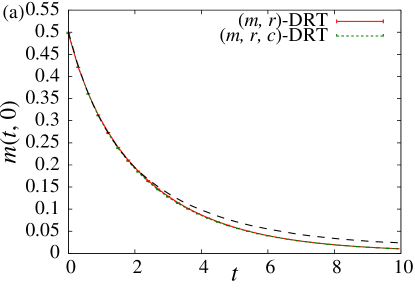
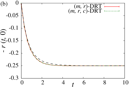
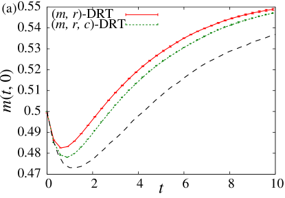
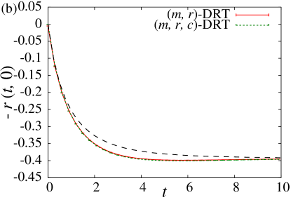
Figure 1: (colour online) Time evolution of (a) $m$ and (b) $-r$ at $T/J=2.0$ and $J_{0}/J=1.0$, whose equilibrium state corresponds to a paramagnetic phase. The solid and dotted lines represent the dynamics theoretically predicted by the $(m,r)$–DRT and $(m,r,c)$–DRT, respectively. The dashed line represents the results of the MC simulation at $N=4096$.

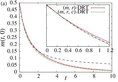
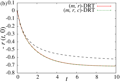
Figure 2: (colour online) Time evolution of (a) $m$ and (b) $-r$ at $T/J=1.0$ and $J_{0}/J=1.5$, whose equilibrium state corresponds to a ferromagnetic phase. The lines are the same as those in Figure 3.

Figure 3: (colour online) Time evolution of (a) $m$ and (b) $-r$ at $T/J=0.5$ and $J_{0}/J=0.0$, whose equilibrium state corresponds to a spin-glass phase. The lines are the same as those in Figure 3. The short time behaviour of the magnetization is shown in the inset of (a).

The evolutional dynamics of $m,~{}r$, and $c$, given by (20)–(22), are solved numerically. The continuous evolutional dynamics are treated discretely in the numerical simulation with a unit step of $\Delta t=0.01$. The changes over time, $\Delta m=m(t+\Delta t)-m(t)$, $\Delta r=r(t+\Delta t)-r(t)$, and $\Delta c=c(t+\Delta t)-c(t)$, are obtained by calculating the noise distribution $D(z,S|\Omega)$ at each time step $t$. To do so, the equations of the variables $(\mu,\mu_{0},\gamma,q,q_{0},q_{t})$, (27)–(29) and (32)–(34), should be solved under the given values of the macroscopic quantities $\Omega(t)=\{m_{0},r_{0},m(t),r(t),c(t)\}$. The conjugates $(\mu,\mu_{0},\gamma)$ and overlaps $(q,q_{0},q_{t})$ are solved alternately until (27)–(29) and (32)–(34) are satisfied simultaneously; the conjugates are implicitly solved by the Newton method based on (27)–(29) under fixed values of the overlaps, and the overlaps are solved recursively based on (32)–(34) under fixed conjugates. The time dependence of the conjugates and overlap parameters are shown in A, which correspond to the time evolution of $m$, $r$ and $c$ shown in this section.

The results of the dynamical equations are compared with a Monte Carlo (MC) simulation for $N=4096$. The MC simulation settings are as follows. The initial spin configuration is randomly generated according to the distribution,

$$P_{S}(S_{i})=\frac{1+m_{0}}{2}\delta_{S_{i},1}+\frac{1-m_{0}}{2}\delta_{S_{i},-1},$$ (50)

and the interaction $\bm{J}$ is generated according to the distribution (2). The MC dynamics are averaged over 1000 realizations of $\bm{J}$ and 100 initial configurations of $\bm{S}$ for each $\bm{J}$. A set of randomly generated spin configurations and interactions generally provides $r(\bm{S})\sim O(N^{-1})$, which is sufficiently small to be regarded as zero at $N=4096$. Therefore, the average over the initial configuration in the MC simulation corresponds to uniform sampling from the subshell characterized by $m_{0}$ and $r_{0}=0$, and the overlap $q_{0}$ at time $t_{w}=0$ is given by $m_{0}^{2}$. In the MC simulation, a randomly chosen $k$-th spin is flipped with probability $w_{k}$ given by (4) every $1/N$ step to match the time scale to that of the DRT.

To clarify the effects of involving the dynamical equation of $c$ into the DRT, the dynamics of $m$ and $r$ are also compared with that of the original DRT [8], in which the subshell is characterized by $m$ and $r$ only. The original DRT and that including the autocorrelation function are denoted by $(m,r)$–DRT and $(m,r,c)$–DRT, respectively. The results in three parameter regions corresponding to paramagnetic, ferromagnetic, and spin-glass phases are shown here.

4.1 Time evolution of the magnetization and randomness energy

The time evolution of $m$ and $-r$ are shown in Figures 3, 3, and 3 for $J_{0}/J=1.0$ and $T/J=2.0$ (paramagnetic phase), $J_{0}/J=1.5$ and $T/J=1.0$ (ferromagnetic phase), and $J_{0}/J=0.0$ and $T/J=0.5$ (spin-glass phase), respectively. The initial condition at $t_{w}=0$ is set to $m_{0}=0.5$ and $r_{0}=0$.

In the paramagnetic phase (Figure 3), the time evolution of $m$ and $r$ in the MC simulation is well described by the $(m,r,c)$-DRT proposed here as well as the original $(m,r)$-DRT. The time evolution does not change significantly by including the autocorrelation function into the DRT formula in the paramagnetic phase.

In the ferromagnetic phase (Figure 3), the time evolution of $m$ predicted by the $(m,r,c)$-DRT is improved from that of the original $(m,r)$-DRT. A discrepancy between the MC simulation and the DRT results appears in early time steps, but it is confirmed that the fixed point of the DRT is coincident with the MC results as $t\to\infty$. The time evolution of $r$ described by the $(m,r,c)$-DRT is almost coincident with that described by the original $(m,r)$-DRT. At sufficiently large $t$, the DRT predicts the correct value of $r$, but the decay to the fixed point at around $2\hskip 3.00003pt\raisebox{1.72218pt}{$<$}\raisebox{-3.01385pt}{$\sim$}\hskip 3.00003ptt\hskip 3.00003pt\raisebox{1.72218pt}{$<$}\raisebox{-3.01385pt}{$\sim$}\hskip 3.00003pt8$ is faster than the MC result.

Figure 3 shows the time evolution of $m$ and $r$ in the spin-glass phase. The short time behaviour of $m$ in the $(m,r,c)$-DRT is slightly improved from that in the $(m,r)$-DRT, as shown in the inset of Figure 3 (a). The fixed point of $m$ in both DRTs is the same, i.e. the RS solution of the SK model. The behaviour of $r$ in both DRTs is similar, but the long time behaviour in the MC simulation is not correctly predicted by either DRT.

To summarize, by taking into account the time evolution of the autocorrelation function, the short time behaviour of the magnetization is improved in the ferromagnetic and spin-glass phases, but there is little effect on the randomness energy in any phase.

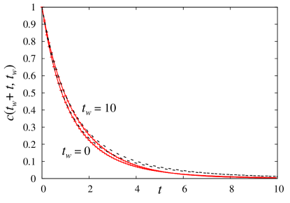
Figure 4: (colour online) Time evolution of the autocorrelation function $c(t_{w}+t,t_{w})$ at $J_{0}/J=1.0$ and $T/J=2.0$. The dashed lines are the results of the MC simulation.

4.2 Time evolution of the autocorrelation function

The time evolution of the autocorrelation function in the $(m,r,c)$-DRT at a waiting time $t_{w}$ is compared to the MC simulation. The autocorrelation $c(t_{w}+t,t_{w})$ for $t_{w}>0$ is calculated according to (14) after resetting $m_{0}=m(t_{w}),~{}r_{0}=r(t_{w})$, and $q_{0}=q(t_{w})$ where $m(t_{w})$ and $r(t_{w})$ are the magnetization and randomness energy at time $t_{w}$ obtained according to the dynamics (12) and (13) with certain initial conditions $m_{0}$ and $r_{0}$. The overlap at time $t_{w}$, $q(t_{w})$, is determined by (32) for given values of $m(t_{w})$ and $r(t_{w})$. Therefore, the non-equilibrium state at time $t_{w}$ is assumed to be specified by three macroscopic quantities: $m(t_{w})$, $r(t_{w})$, and $q(t_{w})$. The time invariance of the autocorrelation function at sufficiently large $t_{w}$ is confirmed over the whole parameter region as $c(t)=\lim_{t_{w}\to\infty}c(t_{w}+t,t_{w})$. When one sets $r_{0}=0$, a solution of the fixed point equations is given by $\rho_{0}=\gamma=0$, as discussed in section 3.3, and in this case the fixed point of the autocorrelation corresponds to $c^{*}=q_{t}=m_{0}\times m^{*}$. Therefore, as $t\to\infty$, if this fixed-point solution is stable, the autocorrelation decreases to zero in the paramagnetic and spin-glass phases irrespective of the value of $m_{0}$. On the other hand, it converges to a finite value given by $m_{0}m^{*}$ in the ferromagnetic phase.

Figure 4 shows the time evolution of $c(t_{w}+t,t_{w})$ at $J_{0}/J=1.0$ and $T/J=2.0$, in which the equilibrium state corresponds to the paramagnetic phase. Both of the results for $t_{w}=0$ and $t_{w}=10$ show good agreement with the results of the MC simulation. The autocorrelation decreases to zero as time increases for any $t_{w}$. In the paramagnetic phase, the solution $c^{*}=q_{t}=0$ is a stable solution of the fixed point equations.

In Figure 5, the time evolution of $c(t_{w}+t,t_{w})$ for $t_{w}=0$ and $t_{w}=10$ are shown for the ferromagnetic phase ($J_{0}/J=1.5$ and $T/J=1.0$). The dynamics of the autocorrelation function are well described by the $(m,r,c)$-DRT for both $t_{w}$ values. As the waiting time $t_{w}$ increases, the relaxation of the autocorrelation appears to be slow. The converged value of $c(t_{w}+t,t_{w})$ corresponds to $m(t_{w})\times m(t_{w}+t)$ for both $t_{w}$ times. In the ferromagnetic phase, $c^{*}=q_{t}=m_{0}m^{*}$ is a stable solution of the fixed point equations where $m^{*}\sim 0.56$ in this parameter region.

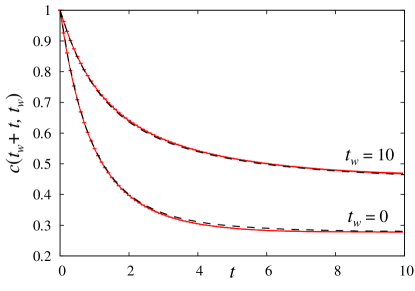
Figure 5: (colour online) Time evolution of the autocorrelation function $c(t_{w}+t,t_{w})$ at $J_{0}/J=1.5$ and $T/J=1.0$. The dashed lines are the results of the MC simulation.

In Figure 6, the time evolution of the autocorrelation function in the spin-glass phase, $J_{0}/J=0$ and $T/J=0.5$, for $t_{w}=0$ and $t_{w}=10$ are shown. At $t_{w}=0$, the short time behaviour of the autocorrelation $c$ is well described by the $(m,r,c)$-DRT, but it deviates from the results of the MC simulation as $t$ increases. The fixed point of the autocorrelation function for $t_{w}=0$ in the spin-glass phase is $c^{*}=0$, as in the paramagnetic phase. As $t_{w}$ increases, the discrepancy between the autocorrelation function in the $(m,r,c)$-DRT and that in the MC simulation widens even in short time steps. In the spin-glass phase, the initial conditions at $t_{w}$, $m_{0}=m(t_{w})$, $r_{0}=r(t_{w})$, and $q_{0}=q(t_{w})$ predicted by the $(m,r,c)$-DRT, are not coincident with the actual values as $t_{w}$ increases, and hence the dynamics after $t_{w}$ in the $(m,r,c)$-DRT do not agree with those in the MC simulation. Generally, DRT predicts a faster relaxation of $m$ and $r$ than the actual relaxation as shown in Figure 3, which indicates that DRT describes the dynamics at time steps later than the actual time. Therefore, the relaxation of the dynamical equation in DRT at $t_{w}>0$ is slower than that in the MC simulation. By setting the initial conditions of $m(t_{w})$ and $r(t_{w})$ in the $(m,r,c)$-DRT to those of the actual values in the MC simulation at $t_{w}$, the short time behaviour of $c(t_{w}+t,t_{w})$ is improved, although there is still a discrepancy between the results. By comparing the results in the paramagnetic and spin-glass phases, it is found that the $(m,r,c)$-DRT can describe the slower relaxation of the autocorrelation function in the spin-glass phase than that in paramagnetic phase.

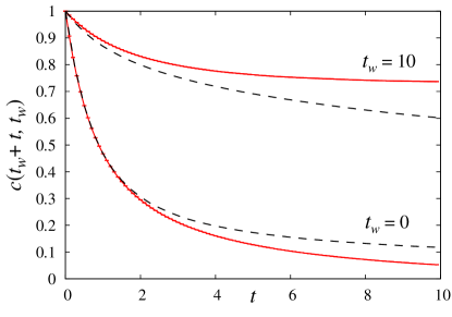
Figure 6: (colour online) Time evolution of the autocorrelation function $c(t_{w}+t,t_{w})$ at $J_{0}/J=0$ and $T/J=0.5$. The dashed lines are the results of the MC simulation.

To characterize the relaxation of the autocorrelation function, it is convenient to introduce the integral relaxation time defined by

$$\tau_{\rm int}(t_{w})=\int_{0}^{t}dt^{\prime}C(t_{w}+t^{\prime},t_{w}).$$ (51)

The tendency of $\tau_{\rm int}(t_{w})$ as $t\to\infty$ is numerically checked by changing the integration range $t$. Figure 7 shows the temperature dependence of $\tau_{\rm int}(t_{w})$ at $J_{0}/J=0$ and $h=0$ for $t_{w}=100$ with integration ranges $t=t_{w}$, $t=5t_{w}$, and $t=10t_{w}$. The spin-glass transition temperature in this parameter region is $T_{c}/J=1$, as indicated by the vertical line in Figure 7. The integral relaxation time in the paramagnetic phase ($T/J>1$) does not depend on the integration range $t$, but it increases in the spin-glass phase ($T/J<1$) as $t$ increases. This means that $\tau_{\rm int}$ diverges as $t\to\infty$ in the spin-glass phase. Around the spin-glass transition temperature, $\tau_{\rm int}$ exhibits a power law behaviour with respect to $T/J-T_{c}/J$ as shown in the inset of Figure 7. In the DRT formulation, $\tau_{\rm int}$ goes to infinity at $T_{c}$ for $\tau_{\rm int}(t_{w})=1.4(T/J-T_{c}/J)^{-0.6}$ at sufficiently large $t_{w}$ and $t$, which indicates that the $(m,r,c)$-DRT can detect the critical slowing down. However, the exponent of 0.6 is smaller than the expected value of 2.0 [20]. The proposed $(m,r,c)$-DRT qualitatively describes slow relaxation in the spin-glass phase and the critical behaviour around the spin-glass transition temperature, but further development is necessary for a more accurate description.

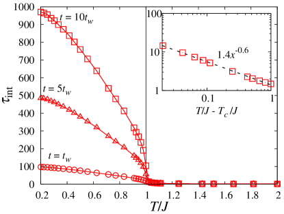
Figure 7: (colour online) The temperature dependence of the integral relaxation time $\tau_{\rm int}$ at $J_{0}/J=0$ and $h=0$ for $t_{w}=100$. The vertical line at $T_{c}/J=1.0$ indicates the spin-glass transition temperature. The inset shows the dependence of $\tau_{\rm int}$ on $(T-T_{c})/J$ with a fitting function denoted by the dashed line.

5 Summary and discussion

In this paper, I have examined the relaxation dynamics in the SK model using DRT and including the autocorrelation function. The joint probability of the microscopic states at times $t_{w}$ and $t_{w}+t$ was introduced, whose time evolution is described by Glauber dynamics. The microscopic states at both times are characterized by macroscopic quantities; the magnetization and energy contributed by randomness at time $t_{w}+t$ denoted by $m$ and $r$, those at time $t_{w}$ denoted by $m_{0}$ and $r_{0}$, as well as the autocorrelation function $c$. Following the DRT procedures, closed dynamical equations were derived based on the self-averaging and subshell equipartitioning assumptions. The dynamical equations are governed by three overlap parameters $q$, $q_{0}$, and $q_{t}$ and the conjugates $\mu,\mu_{0}$, and $\gamma$ under the RS assumption.

The time evolution of $m$ in the $(m,r,c)$-DRT is improved in the ferromagnetic and spin-glass phases compared with $(m,r)$-DRT but that of $r$ does not change significantly in any phase. In the paramagnetic and ferromagnetic phases, the time evolution of the autocorrelation function $c(t_{w}+t,t_{w})$ was well described by the proposed framework even at a finite $t_{w}$. In the spin-glass phase, the short time behaviour of $c(t_{w}+t,t_{w})$ at $t_{w}=0$ was well described by the $(m,r,c)$-DRT, but the theoretical prediction deviated from the MC simulation as the waiting time $t_{w}$ and the difference between the two times $t$ increased. The temperature dependence of $c(t_{w}+t,t_{w})$ was characterized by the integral relaxation time $\tau_{\rm int}$, and it was found that slow relaxation in the spin-glass phase and the critical slowing down are qualitatively described by the current $(m,r,c)$-DRT formulation.

To improve the results in the spin-glass phase, the validity of the assumptions, RS and subshell equipartitioning with some macroscopic quantities, should be discussed. A promising way for the improvement is to introduce a higher-order macroscopic quantity to characterize the subshell as in [18] and RSB [1, 2]. Another straightforward development is to take into account multitime correlations. One can obtain the dynamical equations of the multitime correlation function by starting with a joint probability distribution of the microscopic states at several time steps. In this case, the analytical method that is employed to derive the dynamical equations corresponds to the replica method for a multi-replicated system consisting of spin systems at each time step, which is called real-replica analysis and employed to understand the RSB picture in the equilibrium state [21].

DRT has been developed here to include the dynamical equation of the autocorrelation function defined by the microscopic states at two specific times. From this study, the ability and prospects of DRT for describing the dynamics of random systems has been shown. A modification of the DRT proposed in this paper will provide an analytical description of the experimentally and numerically employed protocols for glassy systems. For example, it is expected that the fluctuation-dissipation relation can be checked in the present formulation by comparing the time evolutions of the susceptibility and autocorrelation function [22]. The current theory is applicable to a $p$-body interaction system; in this case the relationship between bifurcation in dynamical equations and static phase transition associated with RSB should be discussed [23].

Appendix A Overlap and conjugate parameters

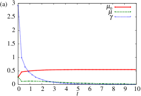
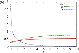
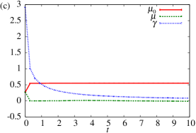
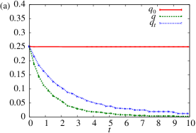
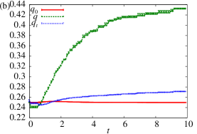
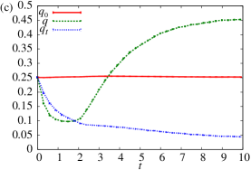
Figure 8: (colour online) Time dependence of the conjugate parameters at (a) $T/J=2.0$ and $J_{0}/J=1.0$, (b) $T/J=1.0$ and $J_{0}/J=1.5$, and (c) $T/J=0.5$ and $J_{0}/J=0.0$ for $t_{w}=0$.

Figure 9: (colour online) Time dependence of the overlap parameters at (a) $T/J=2.0$ and $J_{0}/J=1.0$, (b) $T/J=1.0$ and $J_{0}/J=1.5$, and (c) $T/J=0.5$ and $J_{0}/J=0.0$ for $t_{w}=0$.

To obtain the time evolution of the macroscopic variables, the overlaps $q_{0},q,q_{t}$ and conjugates $\mu_{0},\mu,\gamma$ should be solved at each time step. Figure 9 and 9 show the time dependence of the conjugates and overlap parameters, respectively, at $t_{w}=0$. The initial condition is given by $m_{0}=0.5$ and $r_{0}=0$, and the corresponding time evolution of the macroscopic quantities are shown in section 4. As shown in Figure 9, the conjugate $\gamma$ decreases to 0 with increasing time. As $t\to\infty$, the conjugates $\mu_{0}$ and $\mu$ converges to the values given by $\tanh^{-1}m_{0}$ and $\beta(J_{0}m^{*}+h)$, respectively. The causality that $q_{0}$ takes a constant value (in this case given by $m_{0}^{2}$) is achieved at all time steps by appropriately controlling the conjugates as shown in Figure 9. The overlap between times $t_{w}$ and $t_{w}+t$, $q_{t}$, decreases to zero in the paramagnetic and spin-glass phases and converges to $m_{0}\times m(t)$ in the ferromagnetic phase.

References

References

- [1] Mzard M., Parisi G., and Virasoro M. Spin Glass Theory and Beyond (World Scientific, 1987)
- [2] Nishimori H. Statistical Physics of Spin Glasses and Information Processing: An Introduction (Oxford Univ. Pr., 2001).
- [3] Bray A. J., and Moore M. A. 1980 J. Phys. C 13 L469
- [4] Monasson R. 1995 Phys. Rev. Lett. 75 2847
- [5] Aspelmeier T., Bray A. J., and Moore M. A. 2004 Phys. Rev. Lett. 92 087203
- [6] Vincent E., Hammann J., Ocio M., Bouchaud J.-P., and Cugliandolo L. F. Complex Behaviour of Glassy Systems: Proceedings of the XIV Sitges Conference on Glassy Systems (Springer, 1996)
- [7] Cugliandolo L. F., Kurchan J., and Ritort F. 1994 Phys. Rev. B 49 6331
- [8] Coolen A.C.C., and Sherrington D. 1994 J. Phys. A: Math. Gen. 27 7687
- [9] De Dominicis C. 1978 Phys. Rev. B 18 4913
- [10] Hatchett J. P. L., Wemmenhove B., Prez Castillo I., Nikoletopoulos T., Skantzos N. S., and Coolen A. C. C. 2004 J. Phys. A: Math. Gen. 37 6201
- [11] Tanaka T., and Osawa S. 1998 J. Phys. A: Math. Gen. 31 4197
- [12] Ozeki T., and Nishimori H. 1994 J. Phys. A: Math. Gen. 27 7061
- [13] Amari S., and Maginu K. 1988 Neural Networks 1 63
- [14] Okada M. 1995 Neural Networks 8 833
- [15] Tanaka T., and Okada M. 2005 IEEE Trans. Info. Theory 51 700
- [16] Sompolinsky H., and Zippelius A. 1982 Phys. Rev. B 25 6860
- [17] Cugliandolo L. F., and Kurchan J. 1994 J. Phys. A: Math. Gen. 27 5749
- [18] Laughton S. N., Coolen A.C.C., and Sherrington D. 1996 J. Phys. A: Math. Gen. 29 763
- [19] Glauber R. J. 1963 J. Math. Phys. 4 294
- [20] Kirkpatrick S., and Sherrington D. 1978 Phys. Rev. B 17 4384
- [21] Kurchan J., Parisi G., and Virasoro M. A. 1993 J. Phys. I France 3 1819
- [22] Crisanti A., and Ritort F. 2003 J. Phys. A: Math. Gen. 36 R181
- [23] Sakata A. unpublished.