Self-sustained emission in semi-infinite non-Hermitian systems at the exceptional point

Abstract

Complex potential and non-Hermitian hopping amplitude are building blocks of a non-Hermitian quantum network. Appropriate configuration, such as $\mathcal{PT}$-symmetric distribution, can lead to a full real spectrum. To investigate the underlying mechanism of this phenomenon, we study the phase diagrams of a semi-infinite non-Hermitian systems. They consist of finite non-Hermitian clusters and semi-infinite leads. Based on the analysis of the solutions of the concrete systems, it is shown that they can have full real spectra without any requirements on the symmetry and the wave function within the leads becomes unidirectional plane waves at the exceptional point. This universal dynamical behavior is demonstrated as the persistent emission and reflectionless absorption of wave packets in the typical non-Hermitian systems containing the complex on-site potentials and non-Hermitian hopping amplitudes.

I Introduction

Non-Hermitian Hamiltonians are often employed to describe the open systems due to their features of complex-valued energy and non-preserved particle probability. Recent observations show that a large families of non-Hermitian Hamiltonians can have all eigenvalues real, if the loss and gain are set in a balanced manner, being invariant under the combination of the parity ($\mathcal{P}$) and the time-reversal ($\mathcal{T}$) symmetry. A parity-time ($\mathcal{PT}$) symmetric non-Hermitian quantum theory has been well developed as the complex extension of conventional quantum mechanics Scholtz ; Bender 98 ; Bender 99 ; Dorey 01 ; Bender 02 ; A.M43 ; A.M36 ; A.M ; Jones . Although the condition of the $\mathcal{PT}$ symmetry for a complete real spectrum is weaker ZXZ , it still implies the underlying mechanism can be based on the balance of the loss and gain. However, such an intuitive consideration of the balance needs to be investigated precisely. The concept of the balance should not be simply understood as the conjugate relation of two non-Hermitian subsystems arising from the $\mathcal{PT}$ symmetry. It can not provide physical explanation to the following features about exceptional point: (i) The $\mathcal{PT}$ symmetry of the system can not guarantee the balance of the loss and the gain, or the reality of the energy levels. (ii) The spontaneous symmetry broken states always appear in pairs. Furthermore, this consideration is also related to the precise physical significance of the complex potential and non-Hermitian coupling, which are basic elements for a discrete non-Hermitian system. On the other hand, the purpose of this investigation is not only for the fundamental physics,but also for the application in practice due to the formal equivalence between the quantum Schrödinger equation and the optical wave equation Ruschhaupt ; R. El-Ganainy ; K. G. Makris ; Christodoulides ; Z. H. Musslimani ; S. Klaiman ; S. Longhi ; H. Schomerus ; LonghiLaser ; YDChong ; Keya . Furthermore, the $\mathcal{PT}$ symmetry breaking has been observed in experiments Guo ; Kottos .

In this paper, we investigate semi-infinite non-Hermitian system without $\mathcal{PT}$ symmetry. Based on this, we try to clarify the concept of balance in the non-Hermitian discrete system in the framework of the quantum mechanics rather than a phenomenological description. We show an entirely real spectrum and study the exceptional point of a semi-infinite non-Hermitian system from the dynamical point of view. We show that the wave function within the lead becomes a unidirectional plane wave at the exceptional point. This universal dynamical behavior is demonstrated as the self-sustained emission and reflectionless absorption of wave packets by two typical non-Hermitian clusters containing the complex on-site potential and non-Hermitian hopping amplitude.

This paper is organized as follows. In Section II we analyze the classification of possible solutions and solve two examples to illustrate our main idea. Section III presents the connection between the semi-infinite systems and $\mathcal{PT}$-symmetric systems. Section IV is devoted to the numerical simulation of the wave packet dynamics to demonstrate the phenomena of the persistent emission and reflectionless absorption. Section V is the summary and discussion.

II Semi-infinite system

The discrete non-Hermitian model, with the non-Hermiticity arising from the on-site complex potentials as well as the non-Hermitian hopping amplitude, is a nice testing ground to study the basic features of the non-Hermitian system not only because of its analytical and numerical tractability but also the experimental accessibility. In recent years, fundamental aspects of non-Hermitian continuum systems are studies by using discretization Znojil , as well as the studies on quantum square wells a1 . On the other hand, non-Hermitian quantum models are also investigated, such as tight-binding systems Bendix ; Liang Jin ; Longhi ; Joglekar ; Joglekar1 ; Joglekar2 , spin systems ZXZ ; Korff ; T. Deguchi ; Giorgi ; ZXZ1 , and strongly correlated systems H. Zhong ; L. Jin . Besides the fundamental features of discrete $\mathcal{PT}$-symmetric quantum systems, theoretical research on the quantum dynamics and scattering behaviors in discrete non-Hermitian networks are investigated in a series of papers Znojil2008 ; Stefano ; ZXZ1 ; a2 ; a3 . In experiment, light transport in large-scale temporal lattices is studied in $\mathcal{PT}$-symmetric fiber networks, it is also demonstrated that the $\mathcal{PT}$-symmetric network can act as a unidirectional invisible media a4 . Although many surprising features and possible applications of $\mathcal{PT}$-symmetric are revealed, they are mostly based on the finite systems. In this paper, we intend to study the infinite system.

II.1 Classification of solutions

Here we consider a semi-infinite lead coupled to a non-Hermitian finite cluster. The Hamiltonian is written as

$$H = H_{l}+H_{\text{sub}},$$

$$H_{l} = -J\overset{0}{\sum_{l=-\infty}}(a_{l}^{{\dagger}}a_{l+1}+\text{H.c.}),$$ (1)

$$H_{\text{sub}} = \sum_{i,j=1}^{N_{s}}\kappa_{ij}a_{i}^{{\dagger}}a_{j}.$$

It is noted that $H_{\text{sub}}$ is non-Hermitian, possessing the complex-valued eigen energy, while $H_{l}$ is Hermitian, having complete spectrum $E=-2J\cos\left(k\right)$, $\left(k\in\left[0,2\pi\right)\right)$ and the eigen state $\sin\left(kj\right)a_{j}^{{\dagger}}\left|0\right\rangle$. To investigate the role of the lead in the non-Hermitian $H_{\text{sub}}$, we will consider the whole solution of the Hamiltonian $H$ and analyze its properties.

The eigen state can be expressed as $\left|\psi\right\rangle=\sum_{j=-\infty}^{N_{s}}f^{k}\left(j\right)a_{j}^{{\dagger}}\left|0\right\rangle$. The explicit form of the wave function $f^{k}\left(j\right)$ depends on the structure of $H_{\text{sub}}$. Generally speaking, the solution of $f^{k}\left(j\right)$ can not be obtained exactly even the explicit form of $H_{\text{sub}}$ is given. However, within the lead the wave function is always in the form

$$f^{k}\left(j\leq 0\right)=A_{k}e^{ikj}+B_{k}e^{-ikj},$$ (2)

due to the semi-infinite boundary condition.

The Schrödinger equation has the explicit form

$$-Jf^{k}\left(j-1\right)-Jf^{k}\left(j+1\right)=Ef^{k}\left(j\right),\text{ }\left(j\leq 0\right)$$

$$-Jf^{k}\left(0\right)+\sum_{i=1}^{N_{s}}\kappa_{i1}f^{k}\left(i\right)=Ef^{k}\left(1\right),$$ (3)

$$\sum_{i=1}^{N_{s}}\kappa_{ij}f^{k}\left(i\right)=Ef^{k}\left(j\right),\text{ }\left(j\in\left[2,N_{s}\right]\right)$$

within all the regions. The solutions of $E$ and $f^{k}\left(j\right)$ depend on the structure of the system $H_{\text{sub}}$. Nevertheless, the exclusive geometry of the lead will give some clues to the characteristics of the eigenvalues and eigenfunctions.

In the framework of Bethe ansatz method, all possible solutions within the lead can be classified into three types:

(1) Scattering state wave, the wave function and energy are in the form

$$f_{\text{{SS}}}\left(j\right) = A_{k}e^{ikj}+B_{k}e^{-ikj},\left(k\ \text{is real}\right)$$ (4)

$$E = -2J\cos\left(k\right).$$ (5)

(2) Monotonic damping wave, the wave function and energy are in the form

$$f_{\mathrm{MD}}\left(j\right) = \left(\pm 1\right)^{j}e^{\beta j},\left(\beta<0\right)$$ (6)

$$E = -2J\cosh\left(\beta\right).$$ (7)

(3) Oscillation damping wave, the wave function and energy are in the form

$$f_{\text{{OD}}}\left(j\right) = e^{ikj+\beta j},\left(\beta<0,k\in\left(0,2\pi\right),k\neq\pi\right)$$ (8)

$$E = -2J\left[\cos\left(k\right)\cosh\left(\beta\right)+i\sin\left(k\right)\sinh\left(\beta\right)\right].$$ (9)

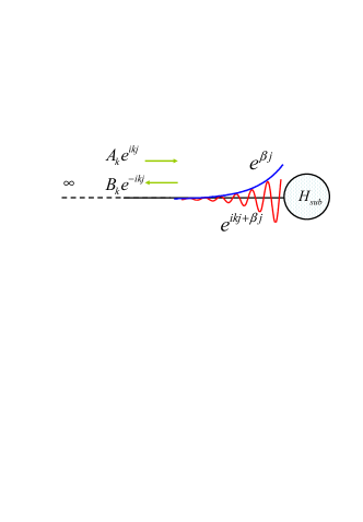
Figure 1: (Color online) Schematic illustration of the configuration of the concerned network and profiles of possible solutions. It consists of a non-Hermitian finite cluster and a semi-infinite chain. The solutions on the lead are threes types: scattering state wave (green), monotonic damping wave (blue) and oscillation damping wave (red).

In Fig. 1, the concerned system and three types of possible solutions within the lead are illustrated schematically. For the case of a hermitian $H_{\text{sub}}$, the solutions are the form of $f_{\text{{SS}}}\left(j\right)$ and $f_{\mathrm{MD}}\left(j\right)$ with $\left|A\right|$ or $\left|B\right|=0$ definitely. In the case of non-Hermitian $H_{\text{sub}}$, $f_{\text{{OD}}}\left(j\right)$ may appear associated with the complex energy level. In case of absence of the solution $f_{\text{{OD}}}\left(j\right)$, full real spectrum achieves, which shows the existence of the stationary states. It indicates that the lead acts as a channel to balance the gain or loss in the system $H_{\text{sub}}$.

At certain points $k_{c}$, the system makes transitions between wavefunctions $f_{\text{{SS}}}\left(j\right)$ and $f_{\mathrm{MD}}\left(j\right)$, as well as between $f_{\text{{SS}}}\left(j\right)$ and $f_{\text{{OD}}}\left(j\right)$. The former transition is actually a switch between real and imaginary $k$, preserving the reality of the eigen energy. Then the transition point locates at $k=0,\pi$, i.e.,

$$f_{\mathrm{MD}}\left(j\right)\overset{\beta=0}{\longrightarrow}\left(\pm 1\right)^{j},$$ (10)

$$f_{\text{{SS}}}\left(j\right)\overset{A\text{ {or} }B=0,\text{ }k=0,\pi}{\longrightarrow}\left(\pm 1\right)^{j},$$ (11)

which usually occurs in the case of Hermitian $H_{\text{sub}}$. The later transition only occurs in a non-Hermitian system, eigen energy switching between real and complex values. In contrast to the above case, the transition point (referred as exceptional point) depends on the structure of the non-Hermitian $H_{\text{sub}}$, i.e.,

$$f_{\text{{OD}}}\left(j\right)\overset{\beta=0}{\longrightarrow}e^{ik_{c}j},$$ (12)

$$f_{\text{{SS}}}\left(j\right)\overset{B=0}{\longrightarrow}e^{ik_{c}j}.$$ (13)

It indicates that a unidirectional plane wave exists in the lead when an appropriate non-Hermitian $H_{\text{sub}}$ is connected. It has both fundamental as well as practical implications. This result reveals the exceptional point from an alternative way: It is the threshold of the balance between the non-Hermitian subcluster and the lead. From a practical perspective, the unidirectional-plane-wave solution at the exceptional point can be used to realize the reflectionless absorption and persistent emission in the experiment. To characterize the probability generation (negative in the case of the dissipation) of the non-Hermitian cluster, we introduce the current operator Caroli

$$\mathcal{\hat{J}}_{j}=-iJ\left(a_{j}^{\dagger}a_{j+1}-a_{j+1}^{\dagger}a_{j}\right),$$ (14)

where $j\in\left[-\infty,0\right]$.

For three types of wave functions $f_{\text{{SS}}}\left(j\right)e^{-iEt}$, $f_{\mathrm{MD}}\left(j\right)e^{-iEt}$ and $f_{\text{{OD}}}\left(j\right)e^{-iEt}$, the corresponding currents can be obtained as

$$\mathcal{J}_{\text{{SS}}} = 2J(\left|A_{k}\right|^{2}-\left|B_{k}\right|^{2})\sin\left(k\right),$$

$$\mathcal{J}_{\text{{MD}}} = 0,$$ (15)

$$\mathcal{J}_{\text{{OD}}} = 2J\sin\left(k\right)e^{2\left[\beta j-2J\sin\left(k\right)\sin\left(\beta\right)t\right]}.$$

We can see that $\mathcal{J}_{\text{{SS}}}$ is time-independent and is conservative along the lead, representing a steady flow or the dynamic balance, while $\mathcal{J}_{\text{{OD}}}$ is non-periodically time-dependent, indicating the unbalance of the state. In other word, the mechanism of the reality of the spectrum is the balance between the source (or drain) and the channel of the probability flow. Then the exceptional point is the threshold of such dynamic balance, corresponding to the unidirectional-plane-wave, i.e., $\left|A_{k}\right|=0$ or $\left|B_{k}\right|=0$. Then the probability generation for the exceptional point is

$$\mathcal{J}_{c}=2J\sin\left(k_{c}\right),$$ (16)

which the sign indicates that the cluster is a source or drain, then it is referred as critical current in this paper. Unlike the situation in traditional quantum mechanics, the magnitude of the current $\mathcal{J}_{c}$ does not represent the absolute current in traditional quantum mechanics because the corresponding eigenstate is not normalized under the Dirac inner product.

We will demonstrate and explain these points through the following illustrative example. We would like to point out that, there is another type of the exceptional point, arising from the transition of two types of wave functions $f_{\text{{OD}}}\left(j\right)$ and $f_{\text{{MD}}}\left(j\right)$, which is beyond our interest.

II.2 Illustrative examples

In this subsection, we investigate two simple exactly solvable systems to illustrate the main idea of this paper. In order to exemplify the above mentioned analysis of relating the wavefunction within the lead and the eigenvalue, we take $H_{\text{sub}}$ to be the simplest non-Hermitian networks to construct two types of exemplified systems. Type I is a uniform chain with a complex potential at one end and type II is a uniform chain with a complex hopping at one end. In the following, we present the analytical results in the framework of above mentioned for the two models in order to perform a comprehensive study.

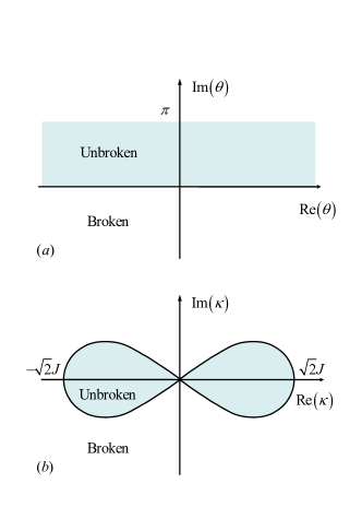
Figure 2: (Color online) Schematic illustration of the phase diagrams in the infinite N system: (a) a uniform chain with a complex potential and (b) with a complex hopping at one end.

II.2.1 Semi-infinite system with complex potential

The type I Hamiltonian has the form

$$H_{\text{CP}}=-J\sum_{j=1}^{\infty}(a_{j}^{\dagger}a_{j+1}+\text{H.c.})+Je^{i\theta}a_{1}^{\dagger}a_{1},$$ (17)

where $\theta$ is a complex number. According to Bethe ansatz method, the wavefunction $f^{k}\left(j\right)$ can be expressed as

$$f^{k}\left(j\right)=A_{k}e^{ikj}+B_{k}e^{-ikj},j\in\left[0,\infty\right)$$ (18)

and the Schrödinger equations for $H_{\text{CP}}$ is

$$-Jf^{k}\left(j+1\right)-Jf^{k}\left(j-1\right) = E_{k}f^{k}\left(j\right),$$ (19)

$$-Jf^{k}\left(2\right) = \left[E_{k}-Je^{i\theta}\right]f^{k}\left(1\right).$$

Submitting $f^{k}\left(j\right)$ into the Schrödinger equation, we have

$$R_{k}=\frac{B_{k}}{A_{k}}=-\frac{1+e^{i\left(\theta+k\right)}}{1+e^{i\left(\theta-k\right)}},$$ (20)

which is the reflection amplitude for the scattering state. Now we are interested in the wavefunction with complex eigen energy. The existence of the solution $f_{\text{{OD}}}\left(j\right)$ requires

$$e^{-ik}=-e^{i\theta}\text{ and Im}\left(k\right)>0,$$ (21)

which lead to $k=\pi-\theta$ with Im$\left(\theta\right)<0$. Then we conclude that there is a unique complex solution within the region Im$\left(\theta\right)<0$ and the system has full real spectrum if the potential is in the rest region. At the boundary, we have

$$\text{Re}\left(\theta_{c}\right)=\theta_{c},$$ (22)

which indicates a circle of radius $J$ in the complex plane. The phase diagram is sketched in Fig. 3 (a). Then the corresponding wavefunction has the form

$$f^{k_{c}}\left(j\right)=e^{i\left(\pi-\theta_{c}\right)j},$$ (23)

which represents a unidirectional plane wave with energy

$$E_{k_{c}}=2J\cos\left(\theta_{c}\right).$$ (24)

Accordingly, the critical current is

$$\mathcal{J}_{c}=2J\sin\left(\theta_{c}\right),$$ (25)

which accords with the intuition that a positive imaginary potential can be a source and a negative imaginary potential can be a drain. However, unlike the situation in traditional quantum mechanics, the magnitude of the current $\mathcal{J}_{c}$ does not represent the absolute current in traditional quantum mechanics because the eigenstate is not normalized under the Dirac inner product.

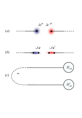
Figure 3: (Color online) Schematic illustration for the non-Hermitian $\mathcal{PT}$-symmetric networks: (a) two separable semi-infinite chains with the complex potential and (b) with the complex hopping at the end. (c) When an arbitrary semi-infinite system and its conjugate counterpart are connected at infinity, a $\mathcal{PT}$-symmetric system are constructed.

Before further discussion of the implication of the obtained result, two distinguishing features need to be mentioned. Firstly, the non-Hermitian system can have full real spectrum even though there is no symmetry required. Secondly, there is only one possible complex energy level rather than complex conjugate pairs. Thus there is no level coalescing occurring at the exceptional point. Both of these differ from that of a finite $\mathcal{PT}$-symmetric system. In the following example, it will be shown that such features are not exclusive to the complex potential.

II.2.2 Semi-infinite system with complex-coupling dimer

The type II Hamiltonian has the form

$$H_{\text{CC}}=-J\sum_{j=2}^{\infty}(a_{j}^{\dagger}a_{j+1}+\text{H.c.})-J\kappa a_{1}^{\dagger}a_{2}-J\kappa a_{2}^{\dagger}a_{1},$$ (26)

which is a different type of the non-Hermitian model in contrast to the type I. Here $\kappa$ is a complex number. In the following, we will perform a parallel investigation with the current Hamiltonian. The Bethe ansatz wave function has the form

$$f^{k}\left(j\right)=\left\{\begin{array}[]{cc}A_{k}e^{ikj}+B_{k}e^{-ikj},&j\in\left[1,\infty\right)\\ C_{k}e^{ikj}+D_{k}e^{-ikj},&j=0\end{array}\right..$$ (27)

Substituting $f^{k}\left(j\right)$ to the Schrödinger equation,

$$-Jf^{k}\left(j-1\right)-Jf^{k}\left(j+1\right) = E_{k}f^{k}\left(j\right),j\in\left[3,\infty\right)$$

$$-J\kappa f^{k}\left(1\right)-Jf^{k}\left(3\right) = E_{k}f^{k}\left(2\right),$$ (28)

$$-J\kappa f^{k}\left(2\right) = E_{k}f^{k}\left(1\right),$$

we obtain the reflection amplitude

$$R_{k}=\frac{B_{k}}{A_{k}}=-\frac{\left(\kappa^{2}-1\right)e^{2ik}-1}{\left(\kappa^{2}-1\right)e^{-2ik}-1}.$$ (29)

The existence of the solution $f_{\text{{OD}}}\left(j\right)$ requires

$$k=\frac{1}{2}i\ln\left(\kappa^{2}-1\right)\text{, }\frac{1}{2}i\ln\left(\kappa^{2}-1\right)+\pi\text{ and Im}\left(k\right)>0.$$ (30)

Similarly, we conclude that there are two complex solutions within the region $\left|\kappa\right|^{4}-2$Re$\left(\kappa^{2}\right)>0$, and the system has full real spectrum if $\kappa$ is in the region $\left|\kappa\right|^{4}-2$Re$\left(\kappa^{2}\right)\leqslant 0$. The phase diagram is sketched in Fig. 2 (b). The boundary can be expressed as

$$\frac{1}{2}\left\{\left[\text{Re}\left(\kappa_{c}\right)\right]^{2}+\left[\text{Im}\left(\kappa_{c}\right)\right]^{2}\right\}^{2}=\left[\text{Re}\left(\kappa_{c}\right)\right]^{2}-\left[\text{Im}\left(\kappa_{c}\right)\right]^{2},$$ (31)

which is a Lemniscate of Bernoulli in the complex plane. Then the corresponding eigen wave functions at the boundary have the form

$$f^{k_{c}}\left(j\right)=\left\{\begin{array}[]{cc}\pm e^{i\left(\varphi/2\right)j},&j\in\left[2,\infty\right)\\ \pm\kappa_{c}^{-1}e^{i\left(\varphi/2\right)j},&j=1\end{array}\right.,$$ (32)

where

$$\tan\varphi=i\frac{\kappa_{c}^{2}-\left(\kappa_{c}^{\ast}\right)^{2}}{\left|\kappa_{c}\right|^{4}-2}$$ (33)

is real. The wave functions $f^{k_{c}}\left(j\right)$ represent unidirectional plane waves with energy $E_{k_{c}}=\pm 2J\cos\left(\varphi/2\right)$, respectively. This indicates that a complex-coupling dimer is a different type of basic element for a discrete non-Hermitian system in comparison with complex potential. There are two eigenstates corresponding to a single exceptional point. In virtue of the critical current $J_{c}=\pm 2J\sin\left(\varphi/2\right)$, one can see that the complex-coupling dimer acts as a source for $J_{c}>0$ but a drain for $J_{c}<0$.

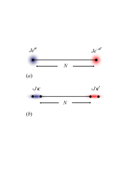
Figure 4: (Color online) Schematic illustration for the non-Hermitian $\mathcal{PT}$-symmetric networks: (a) an uniform chain with a complex potential and (b) with a complex hopping at both sides.

It is noted that both above two examples are not symmetric, which show that the symmetry is not the necessary condition for the occurrence of full real spectrum. The underlying mechanism can be explained as the balance between the source (or drain) and the channel. In this sense, a semi-infinite chain can act as a source (or drain) to balance the original drain (or source). The exceptional point is the threshold of such balance. This point will be elucidated in details in the section III.

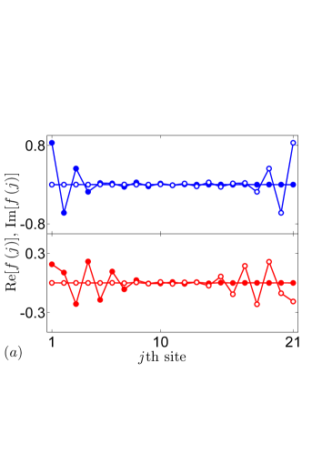
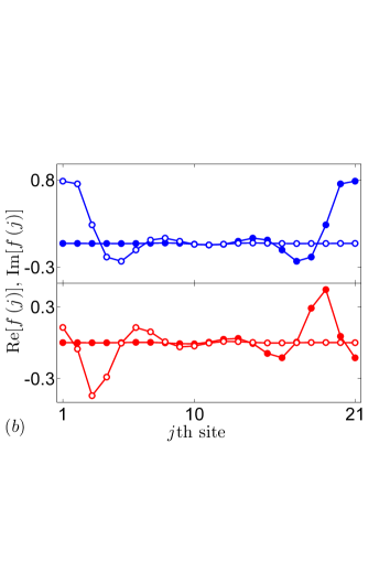
Figure 5: (Color online) Plots of the eigen fuctions of (a) $H_{\text{1}}$ with $\theta=0.4-0.4$i, eigen energy $1.99\pm 0.32$i, and (b) $H_{\text{2}}$ with $\kappa=1+1$i, eigen energy $-1.14\pm 0.71$i, for $N=20$ chain. The blue and red solid (empty) circle indicate the real (imaginary) part of wave functions for the conjugate pairs, respectively. It can be observed that the eigen functions are localized around the non-Hermitian clusters and thus break the $\mathcal{PT}$ symmetry. We also note that two eigen functions of the conjugate pairs are $\mathcal{PT}$-symmetric counterpart to each other.

III Connection between the semi-infinite systems and $\mathcal{PT}$ symmetric systems

So far we have shown that there exist a class of semi-infinite non-Hermitian non-$\mathcal{PT}$ symmetric systems possessing fully real spectra. The occurrence of complex levels in such systems, or quantum transition, is not accompanied by the spontaneous symmetry breaking, but the delocalization-localization transition of wave functions. So it is interesting to consider the connection between the obtained results and the well developed non-Hermitian $\mathcal{PT}$-symmetric quantum mechanics.

III.1 $\mathcal{PT}$ symmetric infinite systems

We start the analysis with the simple configuration, which can constructed from $H_{\text{CP}}$ ($H_{\text{CC}}$) and its $\mathcal{PT}$ counterpart $\mathcal{PT}H_{\text{CP}}\left(\mathcal{PT}\right)^{-1}$ ($\mathcal{PT}H_{\text{CC}}\left(\mathcal{PT}\right)^{-1}$), as sketched in Figs. 3 (a) and (b). Here the action of the parity operator $\mathcal{P}$ is defined as $\mathcal{P}:l\rightarrow-l$ and the time-reversal operator $\mathcal{T}$ as $\mathcal{T}:i\rightarrow-i$. The Hamiltonians are written as

$$H_{\text{CP}}^{\mathcal{PT}} = H_{\text{CP}}+\mathcal{PT}H_{\text{CP}}\left(\mathcal{PT}\right)^{-1}$$

$$= -J\sum_{\begin{subarray}{c}j=-\infty,\\ \left(j\neq-1,0\right)\end{subarray}}^{\infty}(a_{j}^{\dagger}a_{j+1}+\text{H.c.})$$

$$+Je^{i\theta}a_{1}^{\dagger}a_{1}+Je^{-i\theta^{\ast}}a_{-1}^{\dagger}a_{-1}$$

and

$$H_{\text{CC}}^{\mathcal{PT}}=H_{\text{CC}}+\mathcal{PT}H_{\text{CC}}\left(\mathcal{PT}\right)^{-1}$$ (35)

$$=-J\sum_{\begin{subarray}{c}j=-\infty,\\ \left(j\neq-2,\pm 1,0\right)\end{subarray}}^{\infty}(a_{j}^{\dagger}a_{j+1}+\text{H.c.})$$

$$-J\kappa\left(a_{1}^{\dagger}a_{2}+\text{H.c.}\right)-J\kappa^{\ast}\left(a_{-1}^{\dagger}a_{-2}+\text{H.c.}\right).$$

Obviously, they are $\mathcal{PT}$-symmetric and have all features of typical pseudo-Hermitian systems: (i) They have the same phase diagrams in Fig. (2) as their corresponding sub-systems $H_{\text{CP}}$ and $H_{\text{CC}}$. At the exceptional points, two eigen functions coalesce an entire plane wave within the whole space except the $0$th site. (ii) The complex levels come in conjugate pairs. $\mathcal{PT}$-symmetry of the eigen functions break. This toy model shows us the essence of symmetry breaking: the delocalization-localization transition of wave functions in each sub-system. At this point we are ready to move to a more complete description, considering an inseparable system.

We start from the corresponding solutions of the Hamiltonians $H_{\text{CP}}^{{\dagger}}$ and $H_{\text{CC}}^{{\dagger}}$, which actually can be obtained by applying time-reversal operation, i.e., taking complex conjugation for the obtained solutions of the Hamiltonians $H_{\text{CP}}$ and $H_{\text{CC}}$. It is interesting to find that the real eigen-valued solutions between $H_{\text{CP}}$ and $H_{\text{CP}}^{{\dagger}}$ ($H_{\text{CC}}$ and $H_{\text{CC}}^{{\dagger}}$) can match with each other due to the fact that

$$\frac{A_{k}}{B_{k}}=\frac{B_{-k}}{A_{-k}},$$ (36)

for both examples in the Eqs. (20) and (29). In other words, all the real eigen-valued solutions will not change if two systems $H_{\text{CP}}$ and $H_{\text{CP}}^{{\dagger}}$ ($H_{\text{CC}}$ and $H_{\text{CC}}^{{\dagger}}$) are connected at the infinity, as sketched in Fig. 3 (c). It is presumable that the similar situation could occur in finite system, i.e., a semi-infinite non-$\mathcal{PT}$ symmetric system can be regarded as the rudiment of the corresponding finite $\mathcal{PT}$-symmetric system. We will demonstrate this point through the following illustrative examples, which are finite versions of combined $H_{\text{CP}}$ and $H_{\text{CP}}^{{\dagger}}$ ($H_{\text{CC}}$ and $H_{\text{CC}}^{{\dagger}}$). A sketch of such systems are given in Figs. 4 (a) and 4 (b).

III.2 $\mathcal{PT}$ symmetric finite systems

The potential example is a $\mathcal{PT}$ symmetric non-Hermitian $N$-site chain with complex on-site potential at two ends, which has the Hamiltonian

$$H_{\text{1}}=-J\sum_{j=1}^{N-1}(a_{j}^{{\dagger}}a_{j+1}+\text{H.c.})+Je^{i\theta}a_{1}^{{\dagger}}a_{1}+Je^{-i\theta^{\ast}}a_{N}^{{\dagger}}a_{N}\text{.}$$ (37)

It is a $\mathcal{PT}$ symmetric model, i.e., $[\mathcal{PT},H_{\text{1}}]=0$, where the action of the parity operator $\mathcal{P}$ is defined as $\mathcal{P}:l\rightarrow N+1-l$ and the time-reversal operator $\mathcal{T}$ as $\mathcal{T}:i\rightarrow-i$. For infinite $N$, it becomes the combination of the systems $H_{\text{CP}}$ and $H_{\text{CP}}^{{\dagger}}$. For finite $N$, it is an extension version of the model proposed in the previous paper Ref. Liang Jin . By using the standard Bethe ansatz method, the solution is determined by the critical equation

$$\Gamma\left(k\right)=0$$ (38)

where

$$\Gamma\left(k\right) = e^{i\left(\theta-\theta^{\ast}\right)}\sin\left[k(N-1)\right]$$

$$+\sin\left[k(N+1)\right]+2\text{Re}\left(e^{i\theta}\right)\sin\left(kN\right).$$

Accordingly, the exceptional point can be obtained by the equations Liang Jin ; L. Jin

$$\Gamma\left(k_{c}\right)=0\text{ and }\left.\frac{\text{d}\Gamma\left(k\right)}{\text{d}k}\right|_{k=k_{c}}=0.$$ (40)

It is difficult to get the explicit solutions of the Eq. (40) for finite $N$. Nevertheless, the equation about d$\Gamma\left(k\right)/$d$k$ can be reduced to

$$e^{i\left(\theta-\theta^{\ast}\right)}\cos\left[k_{c}(N-1)\right]+\cos\left[k_{c}(N+1)\right]$$ (41)

$$+2\text{Re}\left(e^{i\theta}\right)\cos\left(k_{c}N\right)\approx 0$$

by taking the approximation $N\pm 1\approx N$ in the large $N$ limit. It is easy to find that the existence of real $k_{c}$ solution requires Im$\left(\theta\right)=0$ and $k_{c}=\pi-\theta$. It is in accordance with result in the corresponding semi-infinite system.

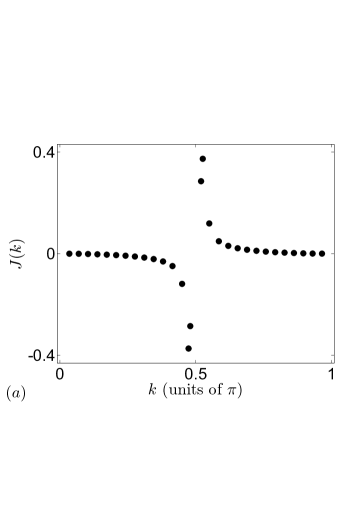
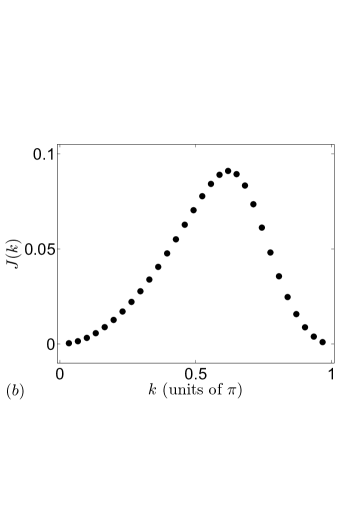
Figure 6: (Color online) Plots of the current $\mathcal{J}\left(k\right)$ for eigenstates of (a) $H_{\text{1}}$ with $\theta=1+0.5$i and (b) $H_{\text{2}}$ with $\kappa=0.3+0.3$i, for $N=30$ chain. As mentioned in the text, the magnitude itself of the current is meaningless. We are interested in the sign of it, which indicates direction of flow, or the location of the source. We note that the sign of the current for $H_{\text{1}}$ are the same and the complex potential can always be source when its imaginary part is positive. This is in accordance with our intuition. Nevertheless, the sign of the current for $H_{\text{2}}$ are different, which indicates that a non-Hermitian dimer cannot be a source or drain absolutely.

The dimer example can be described by the Hamiltonian

$$H_{\text{2}} = -J\sum_{j=2}^{N-2}(a_{j}^{{\dagger}}a_{j+1}+\text{{H.c.}})-J\kappa(a_{1}^{{\dagger}}a_{2}+\text{{H.c.}})$$ (42)

$$+J\kappa^{\ast}\left(a_{N-1}^{{\dagger}}a_{N}+\text{{H.c.}}\right),$$

which corresponds to the combination of two systems $H_{\text{CC}}$ and $H_{\text{CC}}^{{\dagger}}$. By the same procedure as that for $H_{\text{1}}$, we find that the critical equation for finite $N$ is

$$\chi_{2}\sin\left[k\left(N-3\right)\right]+\chi_{1}\sin\left[k\left(N-1\right)\right]$$ (43)

$$-\sin\left[k\left(N+1\right)\right]=0$$

where

$$\chi_{1} = \kappa^{2}+\left(\kappa^{\ast}\right)^{2}-2,$$ (44)

$$\chi_{2} = \chi_{1}-\left|\kappa\right|^{4}+1.$$ (45)

In addition, the exceptional point for large $N$ is determined by the equations

$$2\chi_{2}\cos\left(2k_{c}\right)+\chi_{1}\approx 0$$ (46)

and

$$2\cos\left(2k_{c}\right)-\chi_{1}=0,$$ (47)

which leads to the same results as the Eqs. (31) and (33).

It has been shown by the $\mathcal{PT}$-symmetric quantum theory, beyond the exceptional points the complex levels in both above two models come in conjugate pairs A.M43 and the $\mathcal{PT}$ symmetry of the corresponding eigen functions break. Nevertheless according to our above analysis, the occurrence of the complex level should be accompanied by the delocalization-localization transition of the corresponding wave function. We perform numerical simulation of eigen functions for finite size system to demonstrate this connection. In Fig. 5, we plot the eigenfuctions with complex eigen values including real and imaginary parts for the models $H_{\text{1}}$ and $H_{\text{2}}$, respectively. It shows that the $\mathcal{PT}$ symmetry of all the eigen functions break and are local, which accords with our analysis.

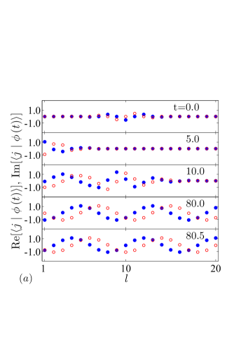
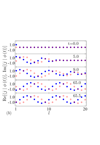
Figure 7: (Color online) The profile of the evolved wave function $\left\langle j\right.\left|\phi\left(t\right)\right\rangle$ for the initial state being (a) an incident Gaussian wavepacket with $k_{0}=-\pi/2$, $N_{A}=10$ and $\alpha=0.5$, and (b) a site state at the left end. We plot the imaginary (blue) and real (red) parts of the amplitudes $\left\langle j\right.\left|\phi\left(t\right)\right\rangle$ of the wave function at instants $t$ with the unit of $1/J$. We see that in both cases, the evolved wave functions tend to the persistent emission of the plane wave with the momentum $k\approx k_{c}=\pi/4$. One can see the plane wave travels to the left and the corresponding phase velocity is $4\sqrt{2}/\pi$ from the subfigures $t=80$ and $t=80.5$ ($t=60$ and $t=60.5$), in the Figs. 7 (a) (7 (b)).

III.3 Current source and drain

The above results are helpful to understand the mechanism of the Hermiticity of a non-Hermitian system. It is well known that the existence of the full real spectra of two above $\mathcal{PT}$ systems is attributed to the balance between the source and drain. Nevertheless, this description cannot provide an explanation for the exceptional point and symmetry breaking since the $\mathcal{PT}$ symmetry of the Hamiltonian seems to maintain such a balance always. Based on the investigations of above two subsections, we can reach the following picture: A finite non-Hermitian cluster can act as a source (or drain), while a semi-infinite lead can act as a tunnel to release the current caused by the source (drain). A semi-infinite lead has its own threshold to carry the current, which is characterized by the onset of complex energy level, or unsteady current. Then the exceptional point in this sense is the threshold of the balance between source (or drain) and the lead. It leads to another signature of the point, delocalization-localization transition of the corresponding wave function.

As for a finite $\mathcal{PT}$-symmetric system in the form $H_{\text{1}}$ and $H_{\text{2}}$, the source and drain is always in balance within the unbroken region. The consistency of the phase diagrams between the finite $\mathcal{PT}$-symmetric system with large $N$ and the corresponding semi-infinite systems shows that the exceptional points are caused by the same mechanism. Then the essence of the symmetry breaking is the unbalance between the source (drain) and the uniform chain, rather than that between source and drain. Loosely speaking, the symmetry breaking is due to that the uniform chain blocks the current from the source and drain. On the other hand, the accordance between the results of these $\mathcal{PT}$ systems with large $N$ and that of semi-infinite systems implies that a lead can act as a multifunctional source (or drain) to match a drain (or source).

We would like to emphasize the difference between two types of non-Hermitian elements, complex on-site potential and non-Hermitian hopping amplitude, by means of the current $\mathcal{J}\left(k\right)=\left\langle k\right|\mathcal{\hat{J}}_{j}\left|k\right\rangle$ for the eigenstate $\left|k\right\rangle$ of the Hamiltonian $H_{\text{1}}$ and $H_{\text{2}}$. In Fig. 6, we plot the current $\mathcal{J}\left(k\right)$ for all the eigenstates $\left|k\right\rangle$ of finite-size systems for $H_{\text{1}}$ and $H_{\text{2}}$. It shows that the signs of the currents are independent of $k$ for $H_{\text{1}}$, but dependent of $k$ for $H_{\text{2}}$. A certain non-Hermitian dimer can be a source or drain for two different eigenstates, which is different from a complex potential.

IV Wavepacket dynamics

In this section we will apply the above theoretical results to simple accessible examples to investigate the dynamic behavior for local initial states. This may provide some insights into the application in practice.

Firstly, we focus on the phenomenon of the persistent emission. Consider an arbitrary local initial state on the lead in the system at the exceptional point. The initial state can always be written in the form

$$\left\langle j\right.\left|\phi\left(t=0\right)\right\rangle=c_{k_{c}}e^{ik_{c}j}+\sum\limits_{k\neq k_{c}}c_{k}\left(e^{ikj}+R_{k}e^{-ikj}\right),$$ (48)

where $\sum\nolimits_{k\neq k_{c}}c_{k}\left(e^{ikj}+R_{k}e^{-ikj}\right)$ represents the superposition of the scattering states with different $k$. It is presumable that the probability of all the scattering states transfers to infinity after a sufficient long time, and then only the unidirectional plane wave survives. To demonstrate and verify this analysis, numerical simulations are performed for two typical initial states: an incoming Gaussion wavepacket and a delta-pulse at the scattering center. A Gaussian wavepacket with momentum $k_{0}$ and initial center $N_{A}$ has the form

$$\left|\psi(k_{0},N_{A})\right\rangle=\frac{1}{\sqrt{\Omega_{0}}}\sum_{j}e^{-\frac{{}^{\alpha^{2}}}{2}(j-N_{A})^{2}}e^{ik_{0}j}\left|j\right\rangle,$$ (49)

where $\Omega_{0}=\sum_{j}e^{-\alpha^{2}(j-N_{A})^{2}}$ is the normalization factor and the half-width of the wavepacket is $2\sqrt{\ln 2}/\alpha$. Here we take $k_{0}=-\pi/2$, $N_{A}=100$ and $\alpha=0.5$. The concerned system is described by the Hamiltonian in the Eq. (37) with $\theta=3\pi/4$, which corresponds to the persistent emission of the plane wave with momentum $k_{c}=\pi/4$. The profiles of the evolved wave functions are plotted in Figs. 7 (a) and 7 (b). One can see the profile of the wave and the corresponding phase velocity from the figures, and after a little long time the evolved wave functions accord with the plane wave of

$$\text{Re}\left(\left\langle j\right.\left|\phi\left(t\right)\right\rangle\right) \sim \cos\left[\left(\pi/4\right)j+2Jt\cos\left(\pi/4\right)\right],$$ (50)

$$\text{Im}\left(\left\langle j\right.\left|\phi\left(t\right)\right\rangle\right) \sim \sin\left[\left(\pi/4\right)j+2Jt\cos\left(\pi/4\right)\right],$$ (51)

within the finite region along the lead, approximately. This result has implications in two aspects: Firstly, we achieve a better understanding of the imaginary potential. We found that a complex potential always corresponds to the wave vector of the unidirectional plane wave, which is determined by Eq. (23). Secondly, it provides a way to measure the complex potential in the experiment.

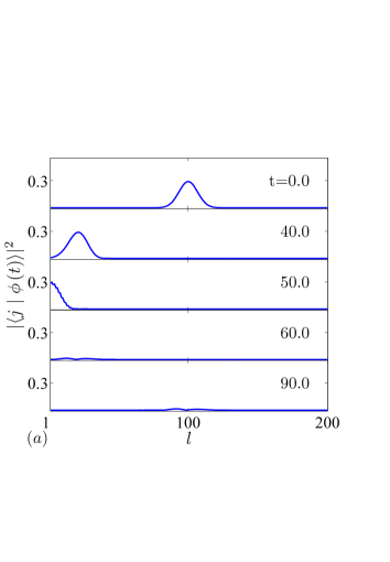
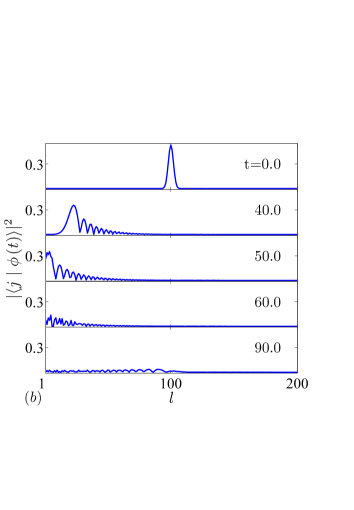
Figure 8: (Color online) The probability distribution of the evolved wave function for the initial state being the incident Gaussian wavepackets with $k_{0}=-\pi/2$, $N_{A}=100$, (a) $\alpha=0.5$, and (b) $\alpha=0.015$. We plot $\left|\left\langle j\right.\left|\phi\left(t\right)\right\rangle\right|^{2}$ at instants $t$ with the unit of $1/J$. We see that in both cases, the reflection coefficients are small, especially for the wider incident wavepacket, which is more close to the plane wave with the momentum $k=k_{c}=\pi/2$.

On the other hand, it is presumable that the reflectionless absorbtion should naturally be reflected in the dynamics of the wavepacket with the momenta around $k_{c}$ due to the continuity of the reflection coefficient in the vicinity of the exceptional point $k_{c}$. Consider an incoming Gaussian wavepacket with momentum $k_{0}=k_{c}$ and initial center $N_{A}$, which can always be written as

$$\left\langle j\right.\left|\psi(k_{c},N_{A})\right\rangle=\frac{1}{\sqrt{\Omega}}\int_{-\pi}^{\pi}e^{-\frac{1}{2\alpha^{2}}\left(k-k_{c}\right)^{2}-iN_{c}\left(k-k_{c}\right)}\text{d}k\left\langle j\right.\left|k\right\rangle,$$ (52)

where $\left\langle j\right.\left|k\right\rangle=e^{ikj}$ denotes the plane wave with momentum $k$, and  $\Omega=\int_{-\pi}^{\pi}e^{-\left(k-k_{c}\right)^{2}/2\alpha^{2}}$d$k$ is the normalization factor. It is a superposition of the plane waves with momenta around $k_{c}$, which have small reflection coefficients. Therefore there is small probability being reflected for the wavepacket. The optimal situations to achieve the reflectionless absorbtion of a wavpacket are determined by the conditions

$$\left|R_{k_{c}}\right|=0\text{, }\left.\frac{\text{d}\left|R_{k}\right|}{\text{d}k}\right|_{k=k_{c}}=0,$$ (53)

which minimizes the reflectional probability. Straightforward derivation indicates that the optimal complex-potential (hopping) scattering center system requires $\theta=\pi/2$ ($\kappa^{2}=1\pm i$) and the momentum of the corresponding reflectionless wave is $k_{c}=\pi/2$ ($\pi/4$).

To demonstrate and verify this analysis, numerical simulations are performed for two initial wavepackets with $k_{0}=-\pi/2$, $N_{A}=100$, $\alpha=0.5$ and $0.15$, respectively. The concerned system is described by the Hamiltonian in the Eq. (37) with $\theta=\pi/2$, which corresponds to the reflectionless plane wave with momentum $k_{c}=\pi/2$. The profiles of the evolved wave functions are plotted in Figs. 8 (a) and 8 (b). The reflection coefficients of the two wavepackets are $0.003$ and $0.035$, respectively. It shows that wider wavepacket leading to lower reflection rate, which accords with the previous theoretical analysis.

V Summary

In summary, the mechanism of the non-Hermiticity of a discrete non-Hermitian system has been investigated in an alternative way. It is shown that the symmetry is not the necessary condition for the occurrence of full real spectrum. The underlying mechanism can be explained as the balance between a non-Hermitian cluster and a semi-infinite chain: the semi-infinite lead can play a complete role to balance a finite non-Hermitian cluster, resulting in a full real spectrum. It is also shown that the threshold of such balance is the exceptional point of the semi-infinite non-Hermitian systems, the occurrence of the corresponding complex eigenstates experienced the delocalization-localization transition. Furthermore, at the exceptional point, the eigen wave function is shown to be a unidirectional plane wave. Practical application of this feature to the dynamics of the wave packet demonstrates the phenomena of the self-sustained emission and reflectionless absorbtion, which could be very useful for the design of quantum devices.

- (1) F. G. Scholtz, H. B. Geyer, and F. J.W.Hahne, Ann. Phys. (NY) 213, 74 (1992).
- (2) C. M. Bender, and S. Boettcher, Phys. Rev. Lett. 80, 5243 (1998).
- (3) C. M. Bender, S. Boettcher, and P. N. Meisinger, J. Math. Phys. 40, 2201 (1999).
- (4) P. Dorey, C. Dunning, and R. Tateo, J. Phys. A: Math. Gen. 34, L391 (2001); P. Dorey, C. Dunning, and R. Tateo, J. Phys. A: Math. Gen. 34, 5679 (2001).
- (5) C. M. Bender, D. C. Brody, and H. F. Jones, Phys. Rev. Lett. 89, 270401 (2002).
- (6) A. Mostafazadeh, J. Math. Phys. 43, 205 (2002); J. Math. Phys. 43, 2814 (2002); J. Math. Phys. 43, 3944 (2002);
- (7) A. Mostafazadeh, J. Phys. A: Math. Gen. 36, 7081 (2003).
- (8) A. Mostafazadeh and A. Batal, J. Phys. A: Math. Gen. 37, 11645 (2004).
- (9) H. F. Jones, J. Phys. A: Math. Gen. 38, 1741 (2005).
- (10) X. Z. Zhang and Z. Song, Phys. Rev. A 87, 012114 (2013).
- (11) A Ruschhaupt, F Delgado and J G Muga, J. Phys. A: Math. Gen. 38, L171 (2005).
- (12) R. El-Ganainy, K. G. Makris, D. N. Christodoulides, and Z. H. Musslimani, Opt. Lett. 32, 2632 (2007).
- (13) K. G. Makris, R. El-Ganainy, D. N. Christodoulides, and Z. H. Musslimani, Phys. Rev. Lett. 100, 103904 (2008).
- (14) K. G. Makris, R. El-Ganainy, D. N. Christodoulides, and Z. H. Musslimani, Phys. Rev. A 81, 063807 (2010).
- (15) Z. H. Musslimani, Phys. Rev. Lett. 100, 030402 (2008).
- (16) S. Klaiman, U. Günther, and N. Moiseyev, Phys. Rev. Lett. 101, 080402 (2008).
- (17) S. Longhi, Phys. Rev. Lett. 103, 123601 (2009).
- (18) H. Schomerus, Phys. Rev. Lett. 104, 233601 (2010).
- (19) S. Longhi, Phys. Rev. A 82, 031801(R) (2010); Phys. Rev. Lett. 105, 013903 (2010).
- (20) Y. D. Chong, Li Ge, Hui Cao and A. D. Stone, Phys. Rev. Lett. 105, 053901 (2010).
- (21) K. Zhou, Z. Guo, J. Wang and S. Liu Opt. Lett. 35, 2928 (2010).
- (22) A. Guo et al., Phys. Rev. Lett. 103, 093902 (2009).
- (23) C. E. Rüter et al., Nat. Phys. 6, 192 (2010); T. Kottos, ibid. 6, 166 (2010); A. Regensburger et al., Nature 488, 167 (2012).
- (24) M. Znojil, Phys. Lett. B 650, 440 (2007); J. Phys. A 40, 13131 (2007); Phys. Rev. A 82, 052113 (2010).
- (25) M. Znojil, J. Math. Phys. 50, 122105 (2009); J. Phys. A: Math. Theor. 44, 075302 (2011), Phys. Lett. A 375, 2503 (2011); M. Znojil and M. Tater, Int. J. Theor. Phys. 50, 982 (2011).
- (26) O. Bendix, R. Fleischmann, T. Kottos and B. Shapiro, Phys. Rev. Lett. 103, 030402 (2009).
- (27) L. Jin and Z. Song, Phys. Rev. A 80, 052107 (2009); Phys. Rev. A 81, 032109 (2010).
- (28) S. Longhi, Phys. Rev. B 82, 041106(R) (2010).
- (29) Y. N. Joglekar, D. Scott, M. Babbey, and A. Saxena, Phys. Rev. A 82, 030103(R) (2010).
- (30) Y. N. Joglekar and A. Saxena, Phys. Rev. A 83, 050101(R) (2011); D. D. Scott and Y. N. Joglekar, Phys. Rev. A 83, 050102(R) (2011); Y. N. Joglekar and J. L. Barnett, Phy. Rev. A 84, 024103 (2011).
- (31) D. D. Scott and Y. N. Joglekar Phys. Rev. A 85, 062105 (2012); J. Phys. A: Math. Theor. 45, 444030 (2012).
- (32) C. Korff and R. Weston, J. Phys. A 40, 8845 (2007); O. A. Castro-Alvaredo and A. Fring, ibid. 42, 465211 (2009).
- (33) T. Deguchi and P. K. Ghosh, J. Phys. A: Math. Theor. 42, 475208 (2009).
- (34) G. L. Giorgi, Phys. Rev. B 82, 052404 (2010).
- (35) X. Z. Zhang, L. Jin, and Z. Song, Phys. Rev. A 85, 012106 (2012).
- (36) H. Zhong, W. Hai, G. Lu, and Z. Li, Phys. Rev. A 84, 013410 (2011).
- (37) L. Jin and Z. Song, Ann. Phys. 330, 142 (2013).
- (38) S. Longhi, Phy. Rev. B 81, 195118 (2010); Phy. Rev. A 82, 032111 (2010).
- (39) M. Znojil, J. Phys. A: Math. Theor. 41, 292002 (2008).
- (40) L. Jin and Z. Song, Phys. Rev. A 81, 022107 (2010); Phys. Rev. A 84, 042116 (2011).
- (41) L. Jin and Z. Song, Phys. Rev. A 85, 012111 (2012); W. H. Hu, L. Jin, Y. Li, and Z. Song, Phys. Rev. A 86, 042110 (2012).
- (42) A. Regensburger, C. Bersch, M.-A. Miri, G. Onishchukov, D. N. Christodoulides and U. Peschel, Nature 488, 167 (2012); M.-A. Miri, A. Regensburger, U. Peschel, D. N. Christodoulides, Phys. Rev. A 86, 023807 (2012).
- (43) C. Caroli, R. Combescot, P. Nozieres, and D. Saint-James, J. Phys. C: Solid St. Phys. 20, 1018 (1965).