Structure estimation for discrete graphical models: Generalized covariance matrices and their inverses

Abstract

We investigate the relationship between the structure of a discrete graphical model and the support of the inverse of a generalized covariance matrix. We show that for certain graph structures, the support of the inverse covariance matrix of indicator variables on the vertices of a graph reflects the conditional independence structure of the graph. Our work extends results that have previously been established only in the context of multivariate Gaussian graphical models, thereby addressing an open question about the significance of the inverse covariance matrix of a non-Gaussian distribution. The proof exploits a combination of ideas from the geometry of exponential families, junction tree theory and convex analysis. These population-level results have various consequences for graph selection methods, both known and novel, including a novel method for structure estimation for missing or corrupted observations. We provide nonasymptotic guarantees for such methods and illustrate the sharpness of these predictions via simulations.

and t1Supported in part by a Hertz Foundation Fellowship and a National Science Foundation Graduate Research Fellowship. t2Supported in part by NSF Grant DMS-09-07632 and Air Force Office of Scientific Research Grant AFOSR-09NL184.

62F12, 68W25, Graphical models, Markov random fields, model selection, inverse covariance estimation, high-dimensional statistics, exponential families, Legendre duality

1 Introduction

Graphical models are used in many application domains, running the gamut from computer vision and civil engineering to political science and epidemiology. In many applications, estimating the edge structure of an underlying graphical model is of significant interest. For instance, a graphical model may be used to represent friendships between people in a social network BanEtal08 or links between organisms with the propensity to spread an infectious disease NewWat99 . It is a classical corollary of the Hammersley–Clifford theorem Grimmett73 , Besag74 , Lau96 that zeros in the inverse covariance matrix of a multivariate Gaussian distribution indicate absent edges in the corresponding graphical model. This fact, combined with various types of statistical estimators suited to high dimensions, has been leveraged by many authors to recover the structure of a Gaussian graphical model when the edge set is sparse (see the papers CaiEtal11 , MeiBuh06 , RavEtal11 , Yua10 and the references therein). Recently, Liu et al. LiuEtal12 and Liu, Lafferty and Wasserman LiuEtal09 introduced the notion of a nonparanormal distribution, which generalizes the Gaussian distribution by allowing for monotonic univariate transformations, and argued that the same structural properties of the inverse covariance matrix carry over to the nonparanormal; see also the related work of Xue and Zou XueZou12 on copula transformations.

However, for non-Gaussian graphical models, the question of whether a general relationship exists between conditional independence and the structure of the inverse covariance matrix remains unresolved. In this paper, we establish a number of interesting links between covariance matrices and the edge structure of an underlying graph in the case of discrete-valued random variables. (Although we specialize our treatment to multinomial random variables due to their widespread applicability, several of our results have straightforward generalizations to other types of exponential families.) Instead of only analyzing the standard covariance matrix, we show that it is often fruitful to augment the usual covariance matrix with higher-order interaction terms. Our main result has an interesting corollary for tree-structured graphs: for such models, the inverse of a generalized covariance matrix is always (block) graph-structured. In particular, for binary variables, the inverse of the usual covariance matrix may be used to recover the edge structure of the tree. We also establish more general results that apply to arbitrary (nontree) graphs, specified in terms of graph triangulations. This more general correspondence exploits ideas from the geometry of exponential families Brown86 , WaiJor08 , as well as the junction tree framework Lauritzen88 , Lau96 .

As we illustrate, these population-level results have a number of corollaries for graph selection methods. Graph selection methods for Gaussian data include neighborhood regression MeiBuh06 , Zhao06 and the graphical Lasso FriEtal08 , RavEtal11 , Rot08 , AspBanGha08 , which corresponds to maximizing an $\ell_{1}$-regularized version of the Gaussian likelihood. Alternative methods for selection of discrete graphical models include the classical Chow–Liu algorithm for trees ChowLiu68 ; techniques based on conditional entropy or mutual information AnaEtal11 , BreEtal08 ; and nodewise logistic regression for discrete graphical models with pairwise interactions JalEtal11 , RavEtal10 . Our population-level results imply that minor variants of the graphical Lasso and neighborhood regression methods, though originally developed for Gaussian data, remain consistent for trees and the broader class of graphical models with singleton separator sets. They also convey a cautionary message, in that these methods will be inconsistent (generically) for other types of graphs. We also describe a new method for neighborhood selection in an arbitrary sparse graph, based on linear regression over subsets of variables. This method is most useful for bounded-degree graphs with correlation decay, but less computationally tractable for larger graphs.

In addition, we show that our methods for graph selection may be adapted to handle noisy or missing data in a seamless manner. Naively applying nodewise logistic regression when observations are systematically corrupted yields estimates that are biased even in the limit of infinite data. There are various corrections available, such as multiple imputation Rub87 and the expectation-maximization (EM) algorithm DemEtal77 , but, in general, these methods are not guaranteed to be statistically consistent due to local optima. To the best of our knowledge, our work provides the first method that is provably consistent under high-dimensional scaling for estimating the structure of discrete graphical models with corrupted observations. Further background on corrupted data methods for low-dimensional logistic regression may be found in Carroll, Ruppert and Stefanski CarEtal95 and Ibrahim et al. IbrEtal05 .

The remainder of the paper is organized as follows. In Section 2, we provide brief background and notation on graphical models and describe the classes of augmented covariance matrices we will consider. In Section 3, we state our main population-level result (Theorem 1) on the relationship between the support of generalized inverse covariance matrices and the edge structure of a discrete graphical model, and then develop a number of corollaries. The proof of Theorem 1 is provided in Section 3.4, with proofs of corollaries and more technical results deferred to the supplementary material LohWai13Sup . In Section 4, we develop consequences of our population-level results in the context of specific methods for graphical model selection. We provide simulation results in Section 4.4 in order to confirm the accuracy of our theoretically-predicted scaling laws, dictating how many samples are required (as a function of graph size and maximum degree) to recover the graph correctly.

2 Background and problem setup

In this section, we provide background on graphical models and exponential families. We then present a simple example illustrating the phenomena and methodology underlying this paper.

2.1 Undirected graphical models

An undirected graphical model or Markov random field (MRF) is a family of probability distributions respecting the structure of a fixed graph. We begin with some basic graph-theoretic terminology. An undirected graph $G=(V,E)$ consists of a collection of vertices $V=\{1,2,\ldots,p\}$ and a collection of unordered vertex pairs $E\subseteq V\times V$. A vertex cutset is a subset $U$ of vertices whose removal breaks the graph into two or more nonempty components [see Figure 1(a)]. A clique is a subset $C\subseteq V$ such that $(s,t)\in E$ for all distinct $s,t\in C$. The cliques in Figure 1(b) are all maximal, meaning they are not properly contained within any other clique. For $s\in V$, we define the neighborhood $N(s):=\{t\in V\mid(s,t)\in E\}$ to be the set of vertices connected to $s$ by an edge.

For an undirected graph $G$, we associate to each vertex $s\in V$ a random variable $X_{s}$ taking values in a space $\mathcal{X}$. For any subset $A\subseteq V$, we define $X_{A}:=\{X_{s},s\in A\}$, and for three subsets of vertices, $A$, $B$ and $U$, we write $X_{A}\perp\!\!\!\perp X_{B}\mid X_{U}$ to mean that the random vector $X_{A}$ is conditionally independent of $X_{B}$ given $X_{U}$. The notion of a Markov random field may be defined in terms of certain Markov properties indexed by vertex cutsets or in terms of a factorization property described by the graph cliques.

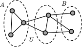
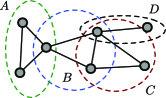
(a)	(b)

Figure 1: (a) Illustration of a vertex cutset: when the set $U$ is removed, the graph breaks into two disjoint subsets of vertices $A$ and $B$. (b) Illustration of maximal cliques, corresponding to fully connected subsets of vertices.

Definition 1 ((Markov property)).

The random vector $X:=(X_{1},\ldots,X_{p})$ is Markov with respect to the graph $G$ if $X_{A}\perp\!\!\!\perp X_{B}\mid X_{U}$ whenever $U$ is a vertex cutset that breaks the graph into disjoint subsets $A$ and $B$.

Note that the neighborhood set $N(s)$ is a vertex cutset for the sets $A=\{s\}$ and $B=V\setminus\{s\cup N(s)\}$. Consequently, $X_{s}\perp\!\!\!\perp X_{V\setminus\{s\cup N(s)\}}\mid X_{N(s)}$. This property is important for nodewise methods for graphical model selection to be discussed later.

The factorization property is defined directly in terms of the probability distribution $q$ of the random vector $X$. For each clique $C$, a clique compatibility function $\psi_{C}$ is a mapping from configurations $x_{C}=\{x_{s},s\in V\}$ of variables to the positive reals. Let $\mathcal{C}$ denote the set of all cliques in $G$.

Definition 2 ((Factorization property)).

The distribution of $X$ factorizes according to $G$ if it may be written as a product of clique functions:

$$q(x_{1},\ldots,x_{p})\propto\prod_{C\in\mathcal{C}}\psi_{C}(x_{C}).$$ (1)

The factorization may always be restricted to maximal cliques of the graph, but it is sometimes convenient to include terms for nonmaximal cliques.

2.2 Graphical models and exponential families

By the Hammersley–Clifford theorem Besag74 , Grimmett73 , Lau96 , the Markov and factorization properties are equivalent for any strictly positive distribution. We focus on such strictly positive distributions, in which case the factorization (1) may alternatively be represented in terms of an exponential family associated with the clique structure of $G$. We begin by defining this exponential family representation for the special case of binary variables ($\mathcal{X}=\{0,1\}$), before discussing a natural generalization to $m$-ary discrete random variables.

Binary variables

For a binary random vector $X\in\{0,1\}^{p}$, we associate with each clique $C$—both maximal and nonmaximal—a sufficient statistic $\mathbb{I}_{C}(x_{C}):=\prod_{s\in C}x_{s}$. Note that $\mathbb{I}_{C}(x_{C})=1$ if and only if $x_{s}=1$ for all $s\in C$, so it is an indicator function for the event $\{x_{s}=1,\ \forall s\in C\}$. In the exponential family, this sufficient statistic is weighted by a natural parameter $\theta_{C}\in\mathbb{R}$, and we rewrite the factorization (1) as

$$q_{\theta}(x_{1},\ldots,x_{p}) = \exp\biggl{\{}\sum_{C\in\mathcal{C}}\theta_{C}\mathbb{I}_{C}(x_{C})-\Phi(\theta)\biggr{\}},$$ (2)

where $\Phi(\theta):=\log\sum_{x\in\{0,1\}^{p}}\exp(\sum_{C\in\mathcal{C}}\theta_{C}\mathbb{I}_{C}(x_{C}))$ is the log normalization constant. It may be verified (cf. Proposition 4.3 of Darroch and Speed DarSpe83 ) that the factorization (2) defines a minimal exponential family, that is, the statistics $\{\mathbb{I}_{C}(x_{C}),C\in\mathcal{C}\}$ are affinely independent. In the special case of pairwise interactions, equation (2) reduces to the classical Ising model:

$$q_{\theta}(x_{1},\ldots,x_{p}) = \exp\biggl{\{}\sum_{s\in V}\theta_{s}x_{s}+\sum_{(s,t)\in E}\theta_{st}x_{s}x_{t}-\Phi(\theta)\biggr{\}}.$$ (3)

The model (3) is a particular instance of a pairwise Markov random field.

Multinomial variables

In order to generalize the Ising model to nonbinary variables, say, $\mathcal{X}=\{0,1,\ldots,m-1\}$, we introduce a larger set of sufficient statistics. We first illustrate this extension for a pairwise Markov random field. For each node $s\in V$ and configuration $j\in\mathcal{X}_{0}:=\mathcal{X}\setminus\{0\}=\{1,2,\ldots,m-1\}$, we introduce the binary-valued indicator function

$$\mathbb{I}_{s;j}(x_{s})=\cases{1,&\quad if $x_{s}=j$,\cr 0,&\quad otherwise.}$$ (4)

We also introduce a vector $\theta_{s}=\{\theta_{s;j},j\in\mathcal{X}_{0}\}$ of natural parameters associated with these sufficient statistics. Similarly, for each edge $(s,t)\in E$ and configuration $(j,k)\in\mathcal{X}^{2}_{0}:=\mathcal{X}_{0}\times\mathcal{X}_{0}$, we introduce the binary-valued indicator function $\mathbb{I}_{st;jk}$ for the event $\{x_{s}=j,x_{t}=k\}$, as well as the collection $\theta_{st}:=\{\theta_{st;jk},(j,k)\in\mathcal{X}^{2}_{0}\}$ of natural parameters. Then any pairwise Markov random field over $m$-ary random variables may be written in the form

$$\qquad q_{\theta}(x_{1},\ldots,x_{p}) = \exp\biggl{\{}\sum_{s\in V}\bigl{\langle}\theta_{s},\mathbb{I}_{s}(x_{s})\bigr{\rangle}+\sum_{(s,t)\in E}\bigl{\langle}\theta_{st},\mathbb{I}_{st}(x_{s},x_{t})\bigr{\rangle}-\Phi(\theta)\biggr{\}},$$ (5)

where we have used the shorthand $\langle\theta_{s},\mathbb{I}_{s}(x_{s})\rangle:=\sum_{j=1}^{m-1}\theta_{s;j}\mathbb{I}_{s;j}(x_{s})$ and $\langle\theta_{st},\break\mathbb{I}_{st}(x_{s},x_{t})\rangle:=\sum_{j,k=1}^{m-1}\theta_{st;jk}\mathbb{I}_{st;jk}(x_{s},x_{t})$. Equation (5) defines a minimal exponential family with dimension $|V|(m-1)+|E|(m-1)^{2}$ DarSpe83 . Note that the family (5) is a natural generalization of the Ising model (3); in particular, when $m=2$, we have a single sufficient statistic $\mathbb{I}_{s;1}(x_{s})=x_{s}$ for each vertex and a single sufficient statistic $\mathbb{I}_{st;11}(x_{s},x_{t})=x_{s}x_{t}$ for each edge. (We have omitted the additional subscript $1$ or $11$ in our earlier notation for the Ising model, since they are superfluous in that case.)

Finally, for a graphical model involving higher-order interactions, we require additional sufficient statistics. For each clique $C\in\mathcal{C}$, we define the subset of configurations

$$\mathcal{X}^{|C|}_{0}:=\underbrace{\mathcal{X}_{0}\times\cdots\times\mathcal{X}_{0}}_{C\ \mathrm{times}}=\bigl{\{}(j_{s},s\in C)\in\mathcal{X}^{|C|}\dvtx j_{s}\neq 0\ \forall s\in C\bigr{\}},$$

a set of cardinality $(m-1)^{|C|}$. As before, $\mathcal{C}$ is the set of all maximal and nonmaximal cliques. For any configuration $J=\{j_{s},s\in C\}\in\mathcal{X}_{0}^{|C|}$, we define the corresponding indicator function

$$\mathbb{I}_{C;J}(x_{C})=\cases{1,&\quad if $x_{C}=J$,\cr 0,&\quad otherwise.}$$ (6)

We then consider the general multinomial exponential family

$$q_{\theta}(x_{1},\ldots,x_{p}) = \exp\biggl{\{}\sum_{C\in\mathcal{C}}\langle\theta_{C},\mathbb{I}_{C}\rangle-\Phi(\theta)\biggr{\}}$$

$$\eqntext{\mbox{for }x_{s}\in\mathcal{X}=\{0,1,\ldots,m-1\}}$$ (8)

with $\langle\theta_{C},\mathbb{I}_{C}(x_{C})\rangle=\sum_{J\in\mathcal{X}_{0}^{|C|}}\theta_{C;J}\mathbb{I}_{C;J}(x_{C})$. Note that our previous models—namely, the binary models (2) and (3), as well as the pairwise multinomial model (5)—are special cases of this general factorization.

Recall that an exponential family is minimal if no nontrivial linear combination of sufficient statistics is almost surely equal to a constant. The family is regular if $\{\theta\dvtx\Phi(\theta)<\infty\}$ is an open set. As will be relevant later, the exponential families described in this section are all minimal and regular DarSpe83 .

2.3 Covariance matrices and beyond

We now turn to a discussion of the phenomena that motivate the analysis of this paper. Consider the usual covariance matrix $\Sigma=\operatorname{cov}(X_{1},\ldots,X_{p})$. When $X$ is jointly Gaussian, it is an immediate consequence of the Hammersley–Clifford theorem that the sparsity pattern of the precision matrix $\Gamma=\Sigma^{-1}$ reflects the graph structure—that is, $\Gamma_{st}=0$ whenever $(s,t)\notin E$. More precisely, $\Gamma_{st}$ is a scalar multiple of the correlation of $X_{s}$ and $X_{t}$ conditioned on $X_{\setminus\{s,t\}}$ (cf. Lauritzen Lau96 ). For non-Gaussian distributions, however, the conditional correlation will be a function of $X_{\setminus\{s,t\}}$, and it is unknown whether the entries of $\Gamma$ have any relationship with the strengths of correlations along edges in the graph.

Nonetheless, it is tempting to conjecture that inverse covariance matrices might be related to graph structure in the non-Gaussian case. We explore this possibility by considering a simple case of the binary Ising model (3).

Example 1.

Consider a simple chain graph on four nodes, as illustrated in Figure 2(a). In terms of the factorization (3), let the node potentials be $\theta_{s}=0.1$ for all $s\in V$ and the edge potentials be $\theta_{st}=2$ for all $(s,t)\in E$. For a multivariate Gaussian graphical model defined on $G$, standard theory predicts that the inverse covariance matrix $\Gamma=\Sigma^{-1}$ of the distribution is graph-structured: $\Gamma_{st}=0$ if and only if $(s,t)\notin E$. Surprisingly, this is also the case for the chain graph with binary variables [see panel (f)]. However, this statement is not true for the single-cycle graph shown in panel (b). Indeed, as shown in panel (g), the inverse covariance matrix has no nonzero entries at all. Curiously, for the more complicated graph in (e), we again observe a graph-structured inverse covariance matrix.

(a) Chain	(b) Single cycle	(c) Edge augmented	(d) With 3-cliques	(e) Dino

$\Gamma_{\mathrm{chain}}=\left[\matrix{9.80&-3.59&0&0\cr-3.59&34.30&-4.77&0\cr 0&-4.77&34.30&-3.59\cr 0&0&-3.59&9.80}\right]$	$\Gamma_{\mathrm{loop}}=\left[\matrix{51.37&-5.37&-0.17&-5.37\cr-5.37&51.37&-5.37&-0.17\cr-0.17&-5.37&51.37&-5.37\cr-5.37&-0.17&-5.37&51.37}\right]$
(f)	(g)

Figure 2: (a)–(e) Different examples of graphical models. (f) Inverse covariance for chain graph in (a). (g) Inverse covariance for single-cycle graph in (b).

Still focusing on the single-cycle graph in panel (b), suppose that instead of considering the ordinary covariance matrix, we compute the covariance matrix of the augmented random vector $(X_{1},X_{2},X_{3},X_{4},X_{1}X_{3})$, where the extra term $X_{1}X_{3}$ is represented by the dotted edge shown in panel (c). The $5\times 5$ inverse of this generalized covariance matrix takes the form

$$\Gamma_{\mathrm{aug}}=10^{3}\times\left[\matrix{1.15&-0.02&1.09&-0.02&-1.14\cr-0.02&0.05&-0.02&0&0.01\cr 1.09&-0.02&1.14&-0.02&-1.14\cr-0.02&0&-0.02&0.05&0.01\cr-1.14&0.01&-1.14&0.01&1.19}\right].$$ (9)

This matrix safely separates nodes $1$ and $4$, but the entry corresponding to the nonedge $(1,3)$ is not equal to zero. Indeed, we would observe a similar phenomenon if we chose to augment the graph by including the edge $(2,4)$ rather than $(1,3)$. This example shows that the usual inverse covariance matrix is not always graph-structured, but inverses of augmented matrices involving higher-order interaction terms may reveal graph structure.

Now let us consider a more general graphical model that adds the 3-clique interaction terms shown in panel (d) to the usual Ising terms. We compute the covariance matrix of the augmented vector

$$\Psi(X) = \{X_{1},X_{2},X_{3},X_{4},X_{1}X_{2},X_{2}X_{3},X_{3}X_{4},$$

$$\hskip 23.0ptX_{1}X_{4},X_{1}X_{3},X_{1}X_{2}X_{3},X_{1}X_{3}X_{4}\}\in\{0,1\}^{11}.$$

Empirically, one may show that the $11\times 11$ inverse $(\operatorname{cov}[\Psi(X)])^{-1}$ respects aspects of the graph structure: there are zeros in position $(\alpha,\beta)$, corresponding to the associated functions $X_{\alpha}=\prod_{s\in\alpha}X_{s}$ and $X_{\beta}=\prod_{s\in\beta}X_{\beta}$, whenever $\alpha$ and $\beta$ do not lie within the same maximal clique. [E.g., this applies to the pairs $(\alpha,\beta)=(\{2\},\{4\})$ and $(\alpha,\beta)=(\{2\},\{1,4\})$.]

The goal of this paper is to understand when certain inverse covariances do (and do not) capture the structure of a graphical model. At its root is the principle that the augmented inverse covariance matrix $\Gamma=\Sigma^{-1}$, suitably defined, is always graph-structured with respect to a graph triangulation. In some cases [e.g., the dino graph in Figure 2(e)], we may leverage the block-matrix inversion formula HorJoh90 , namely,

$$\Sigma_{A,A}^{-1}=\Gamma_{A,A}-\Gamma_{A,B}\Gamma_{B,B}^{-1}\Gamma_{B,A},$$ (10)

to conclude that the inverse of a sub-block of the augmented matrix (e.g., the ordinary covariance matrix) is still graph-structured. This relation holds whenever $A$ and $B$ are chosen in such a way that the second term in equation (10) continues to respect the edge structure of the graph. These ideas will be made rigorous in Theorem 1 and its corollaries in the next section.

3 Generalized covariance matrices and graph structure

We now state our main results on the relationship between the zero pattern of generalized (augmented) inverse covariance matrices and graph structure. In Section 4 to follow, we develop some consequences of these results for data-dependent estimators used in structure estimation.

We begin with some notation for defining generalized covariance matrices, stated in terms of the sufficient statistics previously defined (6). Recall that a clique $C\in\mathcal{C}$ is associated with the collection $\{\mathbb{I}_{C;J},J\in\mathcal{X}_{0}^{|C|}\}$ of binary-valued sufficient statistics. Let $\mathcal{S}\subseteq\mathcal{C}$, and define the random vector

$$\Psi(X;\mathcal{S}) = \bigl{\{}\mathbb{I}_{C;J},J\in\mathcal{X}_{0}^{|C|},C\in\mathcal{S}\bigr{\}},$$ (11)

consisting of all the sufficient statistics indexed by elements of $\mathcal{S}$. As in the previous section, the set $\mathcal{C}$ contains both maximal and nonmaximal cliques.

We will often be interested in situations where $\mathcal{S}$ contains all subsets of a given set. For a subset $A\subseteq V$, let $\operatorname{pow}(A)$ denote the collection of all $2^{|A|}-1$ nonempty subsets of $A$. We extend this notation to $\mathcal{S}$ by defining

$$\operatorname{pow}(\mathcal{S}):=\bigcup_{C\in\mathcal{S}}\operatorname{pow}(C).$$

3.1 Triangulation and block structure

Our first main result concerns a connection between the inverses of generalized inverse covariance matrices associated with the model (2.2) and any triangulation of the underlying graph $G$. The notion of a triangulation is defined in terms of chordless cycles, which are sequences of distinct vertices $\{s_{1},\ldots,s_{\ell}\}$ such that:

• $(s_{i},s_{i+1})\in E$ for all $1\leq i\leq\ell-1$, and also $(s_{\ell},s_{1})\in E$;

• no other nodes in the cycle are connected by an edge.

As an illustration, the $4$-cycle in Figure 2(b) is a chordless cycle.

Definition 3 ((Triangulation)).

Given an undirected graph $G=(V,E)$, a triangulation is an augmented graph $\widetilde{G}=(V,\widetilde{E})$ that contains no chordless cycles of length greater than 3.

Note that a tree is trivially triangulated, since it contains no cycles. On the other hand, the chordless $4$-cycle in Figure 2(b) is the simplest example of a nontriangulated graph. By adding the single edge $(1,3)$ to form the augmented edge set $\widetilde{E}=E\cup\{(1,3)\}$, we obtain the triangulated graph $\widetilde{G}=(V,\widetilde{E})$ shown in panel (c). One may check that the more complicated graph shown in Figure 2(e) is triangulated as well.

Our first result concerns the inverse $\Gamma$ of the matrix $\operatorname{cov}(\Psi(X;\widetilde{\mathcal{C}}))$, where $\widetilde{\mathcal{C}}$ is the set of all cliques arising from some triangulation $\widetilde{G}$ of $G$. For any two subsets $A,B\in\widetilde{\mathcal{C}}$, we write $\Gamma(A,B)$ to denote the sub-block of $\Gamma$ indexed by all indicator statistics on $A$ and $B$, respectively. (Note that we are working with respect to the exponential family representation over the triangulated graph $\widetilde{G}$.) Given our previously-defined sufficient statistics (6), the sub-block $\Gamma(A,B)$ has dimensions $d_{A}\times d_{B}$, where

$$d_{A}:=(m-1)^{|A|}\quad\mbox{and}\quad d_{B}:=(m-1)^{|B|}.$$

For example, when $A=\{s\}$ and $B=\{t\}$, the submatrix $\Gamma(A,B)$ has dimension $(m-1)\times(m-1)$. With this notation, we have the following result:

Theorem 1 ((Triangulation and block graph-structure))

Consider an arbitrary discrete graphical model of the form (2.2), and let $\widetilde{\mathcal{C}}$ be the set of all cliques in any triangulation of $G$. Then the generalized covariance matrix $\operatorname{cov}(\Psi(X;\widetilde{\mathcal{C}}))$ is invertible, and its inverse $\Gamma$ is block graph-structured:

1. [(a)]

2. For any two subsets $A,B\in\widetilde{\mathcal{C}}$ that are not subsets of the same maximal clique, the block $\Gamma(A,B)$ is identically zero.

3. For almost all parameters $\theta$, the entire block $\Gamma(A,B)$ is nonzero whenever $A$ and $B$ belong to a common maximal clique.

In part (b), “almost all” refers to all parameters $\theta$ apart from a set of Lebesgue measure zero. The proof of Theorem 1, which we provide in Section 3.4, relies on the geometry of exponential families Brown86 , WaiJor08 and certain aspects of convex analysis Roc70 , involving the log partition function $\Phi$ and its Fenchel–Legendre dual $\Phi^{*}$. Although we have stated Theorem 1 for discrete variables, it easily generalizes to other classes of random variables. The only difference is the specific choices of sufficient statistics used to define the generalized covariance matrix. This generality becomes apparent in the proof.

To provide intuition for Theorem 1, we consider its consequences for specific graphs. When the original graph is a tree [such as the graph in Figure 2(a)], it is already triangulated, so the set $\widetilde{\mathcal{C}}$ is equal to the edge set $E$, together with singleton nodes. Hence, Theorem 1 implies that the inverse $\Gamma$ of the matrix of sufficient statistics for vertices and edges is graph-structured, and blocks of nonzeros in $\Gamma$ correspond to edges in the graph. In particular, we may apply Theorem 1(a) to the subsets $A=\{s\}$ and $B=\{t\}$, where $s$ and $t$ are distinct vertices with $(s,t)\notin E$, and conclude that the $(m-1)\times(m-1)$ sub-block $\Gamma(A,B)$ is equal to zero.

When $G$ is not triangulated, however, we may need to invert a larger augmented covariance matrix and include sufficient statistics over pairs $(s,t)\notin E$ as well. For instance, the augmented graph shown in Figure 2(c) is a triangulation of the chordless $4$-cycle in panel (b). The associated set of maximal cliques is given by $\overline{\mathcal{C}}=\{(1,2),(2,3),(3,4),(1,4),(1,3)\}$; among other predictions, our theory guarantees that the generalized inverse covariance $\Gamma$ will have zeros in the sub-block $\Gamma(\{2\},\{4\})$.

3.2 Separator sets and graph structure

In fact, it is not necessary to take sufficient statistics over all maximal cliques, and we may consider a slightly smaller augmented covariance matrix. (This simpler type of augmented covariance matrix explains the calculations given in Section 2.3.)

By classical graph theory, any triangulation $\widetilde{G}$ gives rise to a junction tree representation of $G$. Nodes in the junction tree are subsets of $V$ corresponding to maximal cliques of $\widetilde{G}$, and the intersection of any two adjacent cliques $C_{1}$ and $C_{2}$ is referred to as a separator set $S=C_{1}\cap C_{2}$. Furthermore, any junction tree must satisfy the running intersection property, meaning that for any two nodes of the junction tree—say, corresponding to cliques $C$ and $D$—the intersection $C\cap D$ must belong to every separator set on the unique path between $C$ and $D$. The following result shows that it suffices to construct generalized covariance matrices augmented by separator sets:

Corollary 1.

Let $\mathcal{S}$ be the set of separator sets in any triangulation of $G$, and let $\Gamma$ be the inverse of $\operatorname{cov}(\Psi(X;V\cup\operatorname{pow}(\mathcal{S})))$. Then $\Gamma(\{s\},\{t\})=0$ whenever $(s,t)\notin\widetilde{E}$.

Note that $V\cup\operatorname{pow}(\mathcal{S})\subseteq\widetilde{\mathcal{C}}$, and the set of sufficient statistics considered in Corollary 1 is generally much smaller than the set of sufficient statistics considered in Theorem 1. Hence, the generalized covariance matrix of Corollary 1 has a smaller dimension than the generalized covariance matrix of Theorem 1, which becomes significant when we consider exploiting these population-level results for statistical estimation.

The graph in Figure 2(c) of Example 1 and the associated matrix in equation (9) provide a concrete example of Corollary 1 in action. In this case, the single separator set in the triangulation is $\{1,3\}$, so when $\mathcal{X}=\{0,1\}$, augmenting the usual covariance matrix with the additional sufficient statistic $\mathbb{I}_{13;11}(x_{1},x_{3})=x_{1}x_{3}$ and taking the inverse yields a graph-structured matrix. Indeed, since $(2,4)\notin\widetilde{E}$, we observe that $\Gamma_{\mathrm{aug}}(2,4)=0$ in equation (9), consistent with the result of Corollary 1.

Although Theorem 1 and Corollary 1 are clean population-level results, however, forming an appropriate augmented covariance matrix requires prior knowledge of the graph, namely, which edges are involved in a suitable triangulation. This is infeasible in settings where the goal is to recover the edge structure of the graph. Corollary 1 is most useful for edge recovery when $G$ admits a triangulation with only singleton separator sets, since then $V\cup\operatorname{pow}(\mathcal{S})=V$. In particular, this condition holds when $G$ is a tree. The following corollary summarizes our result:

Corollary 2.

For any graph with singleton separator sets, the inverse $\Gamma$ of the covariance matrix $\operatorname{cov}(\Psi(X;V))$ of vertex statistics is graph-structured. (This class includes trees as a special case.)

In the special case of binary variables, we have $\Psi(X;V)=(X_{1},\ldots,X_{p})$, so Corollary 2 implies that the inverse of the ordinary covariance matrix $\operatorname{cov}(X)$ is graph-structured. For $m$-ary variables, $\operatorname{cov}(\Psi(X;V))$ is a matrix of dimensions $(m-1)p\times(m-1)p$ involving indicator functions for each variable. Again, we may relate this corollary to Example 1—the inverse covariance matrices for the tree graph in panel (a) and the dino graph in panel (e) are exactly graph-structured. Although the dino graph is not a tree, it possesses the nice property that the only separator sets in its junction tree are singletons.

Corollary 1 also guarantees that inverse covariances may be partially graph-structured, in the sense that $\Gamma(\{s\},\{t\})=0$ for any pair of vertices $(s,t)$ separable by a singleton separator set, where $\Gamma=(\operatorname{cov}(\Psi(X;V)))^{-1}$. This is because for any such pair $(s,t)$, we may form a junction tree with two nodes, one containing $s$ and one containing $t$, and apply Corollary 1. Indeed, the matrix $\Gamma$ defined over singleton vertices is agnostic to which triangulation we choose for the graph.

In settings where there exists a junction tree representation of the graph with only singleton separator sets, Corollary 2 has a number of useful implications for the consistency of methods that have traditionally only been applied for edge recovery in Gaussian graphical models: for tree-structured discrete graphs, it suffices to estimate the support of $(\operatorname{cov}(\Psi(X;V)))^{-1}$ from the data. We will review methods for Gaussian graphical model selection and describe their analogs for discrete tree graphs in Sections 4.1 and 4.2.

3.3 Generalized covariances and neighborhood structure

Theorem 1 also has a corollary, that is, relevant for nodewise neighborhood selection approaches to graph selection MeiBuh06 , RavEtal11 , which are applicable to graphs with arbitrary topologies. Nodewise methods use the basic observation that recovering the edge structure of $G$ is equivalent to recovering the neighborhood set $N(s)=\{t\in V\dvtx(s,t)\in E\}$ for each vertex $s\in V$. For a given node $s\in V$ and positive integer $d$, consider the collection of subsets

$$\mathcal{S}(s;d):=\bigl{\{}U\subseteq V\setminus\{s\},|U|=d\bigr{\}}.$$

The following corollary provides an avenue for recovering $N(s)$ based on the inverse of a certain generalized covariance matrix:

Corollary 3 ((Neighborhood selection)).

For any graph and node $s\in V$ with $\deg(s)\leq d$, the inverse $\Gamma$ of the matrix $\operatorname{cov}(\Psi(X;\{s\}\cup\operatorname{pow}(\mathcal{S}(s;d))))$ is $s$-block graph-structured, that is, $\Gamma(\{s\},B)=0$ whenever $\{s\}\neq B\subsetneq N(s)$. In particular, $\Gamma(\{s\},\{t\})=0$ for all vertices $t\notin N(s)$.

Note that $\operatorname{pow}(\mathcal{S}(s;d))$ is the set of subsets of all candidate neighborhoods of $s$ of size $d$. This result follows from Theorem 1 (and the related Corollary 1) by constructing a particular junction tree for the graph, in which $s$ is separated from the rest of the graph by $N(s)$. Due to the well-known relationship between the rows of an inverse covariance matrix and linear regression coefficients MeiBuh06 , Corollary 3 motivates the following neighborhood-based approach to graph selection: for a fixed vertex $s\in V$, perform a single linear regression of $\Psi(X;\{s\})$ on the vector $\Psi(X;\operatorname{pow}(\mathcal{S}(s;d)))$. Via elementary algebra and an application of Corollary 3, the resulting regression vector will expose the neighborhood $N(s)$ in an arbitrary discrete graphical model; that is, the indicators $\Psi(X;\{t\})$ corresponding to $X_{t}$ will have a nonzero weight only if $t\in N(s)$. We elaborate on this connection in Section 4.2.

3.4 Proof of Theorem 1

We now turn to the proof of Theorem 1, which is based on certain fundamental correspondences arising from the theory of exponential families Barndorff78 , Brown86 , WaiJor08 . Recall that our exponential family (2.2) has binary-valued indicator functions (6) as its sufficient statistics. Let $D$ denote the cardinality of this set and let $\mathbb{I}\dvtx\mathcal{X}^{p}\rightarrow\{0,1\}^{D}$ denote the multivariate function that maps each configuration $x\in\mathcal{X}^{p}$ to the vector $\mathbb{I}(x)$ obtained by evaluating the $D$ indicator functions on $x$. Using this notation, our exponential family may be written in the compact form $q_{\theta}(x)=\exp\{\langle\theta,\mathbb{I}(x)\rangle-\Phi(\theta)\}$, where

$$\bigl{\langle}\theta,\mathbb{I}(x)\bigr{\rangle} = \sum_{C\in\mathcal{C}}\bigl{\langle}\theta_{C},\mathbb{I}_{C}(x)\bigr{\rangle}=\sum_{C\in\mathcal{C}}\sum_{J\in\mathcal{X}_{0}^{|C|}}\theta_{C;J}\mathbb{I}_{C;J}(x_{C}).$$

Since this exponential family is known to be minimal, we are guaranteed DarSpe83 that

$$\nabla\Phi(\theta)=\mathbb{E}_{\theta}\bigl{[}\mathbb{I}(X)\bigr{]}\quad\mbox{and}\quad\nabla^{2}\Phi(\theta)=\operatorname{cov}_{\theta}\bigl{[}\mathbb{I}(X)\bigr{]},$$

where $\mathbb{E}_{\theta}$ and $\operatorname{cov}_{\theta}$ denote (resp.) the expectation and covariance taken under the density $q_{\theta}$ Brown86 , WaiJor08 . The conjugate dual Roc70 of the cumulant function is given by

$$\Phi^{*}(\mu):=\sup_{\theta\in\mathbb{R}^{D}}\bigl{\{}\langle\mu,\theta\rangle-\Phi(\theta)\bigr{\}}.$$

The function $\Phi^{*}$ is always convex and takes values in $\mathbb{R}\cup\{+\infty\}$. From known results WaiJor08 , the dual function $\Phi^{*}$ is finite only for $\mu\in\mathbb{R}^{D}$ belonging to the marginal polytope

$$\mathcal{M}:=\biggl{\{}\mu\in\mathbb{R}^{p}\biggm{|}\exists\mbox{ some density $q$ s.t. }\sum_{x}q(x)\mathbb{I}(x)=\mu\biggr{\}}.$$ (12)

The following lemma, proved in the supplementary material LohWai13Sup , provides a connection between the covariance matrix and the Hessian of $\Phi^{*}$:

Lemma 1.

Consider a regular, minimal exponential family, and define $\mu=\mathbb{E}_{\theta}[\mathbb{I}(X)]$ for any fixed $\theta\in\Omega=\{\theta\dvtx\Phi(\theta)<\infty\}$. Then

$$\bigl{(}\operatorname{cov}_{\theta}\bigl{[}\mathbb{I}(X)\bigr{]}\bigr{)}^{-1} = \nabla^{2}\Phi^{*}(\mu).$$ (13)

Note that the minimality and regularity of the family implies that $\operatorname{cov}_{\theta}[\mathbb{I}(X)]$ is strictly positive definite, so the matrix is invertible.

For any $\mu\in\operatorname{int}(\mathcal{M})$, let $\theta(\mu)\in\mathbb{R}^{D}$ denote the unique natural parameter $\theta$ such that $\nabla\Phi(\theta)=\mu$. It is known WaiJor08 that the negative dual function $-\Phi^{*}$ is linked to the Shannon entropy via the relation

$$-\Phi^{*}(\mu) = H\bigl{(}q_{\theta(\mu)}(x)\bigr{)}=-\sum_{x\in\mathcal{X}^{p}}q_{\theta(\mu)}(x)\log q_{\theta(\mu)}(x).$$ (14)

In general, expression (14) does not provide a straightforward way to compute $\nabla^{2}\Phi^{*}$, since the mapping $\mu\mapsto\theta(\mu)$ may be extremely complicated. However, when the exponential family is defined with respect to a triangulated graph, $\Phi^{*}$ has an explicit closed-form representation in terms of the mean parameters $\mu$. Consider a junction tree triangulation of the graph, and let $(\overline{\mathcal{C}},\mathcal{S})$ be the collection of maximal cliques and separator sets, respectively. By the junction tree theorem Lauritzen88 , WaiJor08 , KolFri09 , we have the factorization

$$q(x_{1},\ldots,x_{p})=\frac{\prod_{C\in\overline{\mathcal{C}}}q_{C}(x_{C})}{\prod_{S\in\mathcal{S}}q_{S}(x_{S})},$$ (15)

where $q_{C}$ and $q_{S}$ are the marginal distributions over maximal clique $C$ and separator set $S$. Consequently, the entropy may be decomposed into the sum

$$H(q) = -\sum_{x\in\mathcal{X}^{p}}q(x)\log q(x)=\sum_{C\in\overline{\mathcal{C}}}H_{C}(q_{C})-\sum_{S\in\mathcal{S}}H_{S}(q_{S}),$$ (16)

where we have introduced the clique- and separator-based entropies

$$H_{S}(q_{S}):=-\sum_{x_{S}\in\mathcal{X}^{|S|}}q_{S}(x_{S})\log q_{S}(x_{S})$$

and

$$H_{C}(q_{C}):=-\sum_{x_{C}\in\mathcal{X}^{|C|}}q_{C}(x_{C})\log q_{C}(x_{C}).$$

Given our choice of sufficient statistics (6), we show that $q_{C}$ and $q_{S}$ may be written explicitly as “local” functions of mean parameters associated with $C$ and $S$. For each subset $A\subseteq V$, let $\mu_{A}\in(m-1)^{|A|}$ be the associated collection of mean parameters, and let

$$\mu_{\operatorname{pow}(A)}:=\{\mu_{B}\mid\varnothing\neq B\subseteq A\}$$

be the set of mean parameters associated with all nonempty subsets of $A$. Note that $\mu_{\operatorname{pow}(A)}$ contains a total of $\sum_{k=1}^{|A|}{|A|\choose k}(m-1)^{k}=m^{|A|}-1$ parameters, corresponding to the number of degrees of freedom involved in specifying a marginal distribution over the random vector $x_{A}$. Moreover, $\mu_{\operatorname{pow}(A)}$ uniquely determines the marginal distribution $q_{A}$:

Lemma 2.

For any marginal distribution $q_{A}$ in the $m^{|A|}$-dimensional probability simplex, there is a unique mean parameter vector $\mu_{\operatorname{pow}(A)}$ and matrix $M_{A}$ such that $q_{A}=M_{A}\cdot\mu_{\operatorname{pow}(A)}$.

For the proof, see the supplementary material LohWai13Sup .

We now combine the dual representation (14) with the decomposition (16), along with the matrices $\{M_{C},M_{S}\}$ from Lemma 2, to conclude that

$$-\Phi^{*}(\mu) = \sum_{C\in\overline{\mathcal{C}}}H_{C}\bigl{(}M_{C}\bigl{(}\mu_{\operatorname{pow}(C)}\bigr{)}\bigr{)}-\sum_{S\in\mathcal{S}}H_{S}\bigl{(}M_{S}\bigl{(}\mu_{\operatorname{pow}(S)}\bigr{)}\bigr{)}.$$ (17)

Now consider two subsets $A,B\in\widetilde{\mathcal{C}}$ that are not contained in the same maximal clique. Suppose $A$ is contained within maximal clique $C$. Differentiating expression (17) with respect to $\mu_{A}$ preserves only terms involving $q_{C}$ and $q_{S}$, where $S$ is any separator set such that $A\subseteq S\subseteq C$. Since $B\subsetneq C$, we clearly cannot have $B\subseteq S$. Consequently, all cross-terms arising from the clique $C$ and its associated separator sets vanish when we take a second derivative with respect to $\mu_{B}$. Repeating this argument for any other maximal clique $C^{\prime}$ containing $A$ but not $B$, we have $\frac{\partial^{2}\Phi^{*}}{\partial\mu_{A}\,\partial\mu_{B}}(\mu)=0$. This proves part (a).

Turning to part (b), note that if $A$ and $B$ are in the same maximal clique, the expression obtained by taking second derivatives of the entropy results in an algebraic expression with only finitely many solutions in the parameters $\mu$ (consequently, also $\theta$). Hence, assuming the $\theta$’s are drawn from a continuous distribution, the corresponding values of the block $\Gamma(A,B)$ are a.s. nonzero.

4 Consequences for graph structure estimation

Moving beyond the population level, we now state and prove several results concerning the statistical consistency of different methods—both known and some novel—for graph selection in discrete graphical models, based on i.i.d. draws from a discrete graph. For sparse Gaussian models, existing methods that exploit sparsity of the inverse covariance matrix fall into two main categories: global graph selection methods (e.g., AspBanGha08 , FriEtal08 , Rot08 , RavEtal11 ) and local (nodewise) neighborhood selection methods MeiBuh06 , Zhao06 . We divide our discussion accordingly.

4.1 Graphical Lasso for singleton separator graphs

We begin by describing how a combination of our population-level results and some concentration inequalities may be leveraged to analyze the statistical behavior of log-determinant methods for discrete graphical models with singleton separator sets, and suggest extensions of these methods when observations are systematically corrupted by noise or missing data. Given a $p$-dimensional random vector $(X_{1},\ldots,X_{p})$ with covariance $\Sigma^{*}$, consider the estimator

$$\widehat{\Theta}\in\arg\min_{\Theta\succeq 0}\biggl{\{}\operatorname{trace}(\widehat{\Sigma}\Theta)-\log\det(\Theta)+\lambda_{n}\sum_{s\neq t}|\Theta_{st}|\biggr{\}},$$ (18)

where $\widehat{\Sigma}$ is an estimator for $\Sigma^{*}$. For multivariate Gaussian data, this program is an $\ell_{1}$-regularized maximum likelihood estimate known as the graphical Lasso and is a well-studied method for recovering the edge structure in a Gaussian graphical model BanEtal08 , FriEtal08 , YuaLin07 , Rot08 . Although the program (18) has no relation to the MLE in the case of a discrete graphical model, it may still be useful for estimating $\Theta^{*}:=(\Sigma^{*})^{-1}$. Indeed, as shown in Ravikumar et al. RavEtal11 , existing analyses of the estimator (18) require only tail conditions such as sub-Gaussianity in order to guarantee that the sample minimizer is close to the population minimizer. The analysis of this paper completes the missing link by guaranteeing that the population-level inverse covariance is in fact graph-structured. Consequently, we obtain the interesting result that the program (18)—even though it is ostensibly derived from Gaussian considerations—is a consistent method for recovering the structure of any binary graphical model with singleton separator sets.

In order to state our conclusion precisely, we introduce additional notation. Consider a general estimate $\widehat{\Sigma}$ of the covariance matrix $\Sigma$ such that

$$\mathbb{P}\biggl{[}\bigl{\|}\widehat{\Sigma}-\Sigma^{*}\bigr{\|}_{\max}\geq\varphi\bigl{(}\Sigma^{*}\bigr{)}\sqrt{\frac{\log p}{n}}\biggr{]} \leq c\exp\bigl{(}-\psi(n,p)\bigr{)}$$ (19)

for functions $\varphi$ and $\psi$, where $\|\cdot\|_{\max}$ denotes the elementwise $\ell_{\infty}$-norm. In the case of fully-observed i.i.d. data with sub-Gaussian parameter $\sigma^{2}$, where $\widehat{\Sigma}=\frac{1}{n}\sum_{i=1}^{n}x_{i}x_{i}^{T}-\bar{x}\bar{x}{}^{T}$ is the usual sample covariance, this bound holds with $\varphi(\Sigma^{*})=\sigma^{2}$ and $\psi(n,p)=c^{\prime}\log p$.

As in past analysis of the graphical Lasso RavEtal11 , we require a certain mutual incoherence condition on the true covariance matrix $\Sigma^{*}$ to control the correlation of nonedge variables with edge variables in the graph. Let $\Gamma^{*}=\Sigma^{*}\otimes\Sigma^{*}$, where $\otimes$ denotes the Kronecker product. Then $\Gamma^{*}$ is a $p^{2}\times p^{2}$ matrix indexed by vertex pairs. The incoherence condition is given by

$$\max_{e\in S^{c}}\bigl{\|}\Gamma^{*}_{eS}\bigl{(}\Gamma^{*}_{SS}\bigr{)}^{-1}\bigr{\|}_{1}\leq 1-\alpha,\qquad\alpha\in(0,1],$$ (20)

where $S:=\{(s,t)\dvtx\Theta^{*}_{st}\neq 0\}$ is the set of vertex pairs corresponding to nonzero entries of the precision matrix $\Theta^{*}$, equivalently, the edge set of the graph, by our theory on tree-structured discrete graphs. For more intuition on the mutual incoherence condition, see Ravikumar et al. RavEtal11 .

With this notation, our global edge recovery algorithm proceeds as follows:

Algorithm 1 ((Graphical Lasso)).

1. Form a suitable estimate $\widehat{\Sigma}$ of the true covariance matrix $\Sigma$.

2. Optimize the graphical Lasso program (18) with parameter $\lambda_{n}$, and denote the solution by $\widehat{\Theta}$.

3. Threshold the entries of $\widehat{\Theta}$ at level $\tau_{n}$ to obtain an estimate of $\Theta^{*}$.

It remains to choose the parameters $(\lambda_{n},\tau_{n})$. In the following corollary, we will establish statistical consistency of $\widehat{\Theta}$ under the following settings:

$$\lambda_{n}\geq\frac{c_{1}}{\alpha}\sqrt{\frac{\log p}{n}},\qquad\tau_{n}=c_{2}\biggl{\{}\frac{c_{1}}{\alpha}\sqrt{\frac{\log p}{n}}+\lambda_{n}\biggr{\}},$$ (21)

where $\alpha$ is the incoherence parameter in inequality (20) and $c_{1},c_{2}$ are universal positive constants. The following result applies to Algorithm 1 when $\widehat{\Sigma}$ is the sample covariance matrix and $(\lambda_{n},\tau_{n})$ are chosen as in equations (21):

Corollary 4.

Consider an Ising model (3) defined by an undirected graph with singleton separator sets and with degree at most $d$, and suppose that the mutual incoherence condition (20) holds. With $n\succsim d^{2}\log p$ samples, there are universal constants $(c,c^{\prime})$ such that with probability at least $1-c\exp(-c^{\prime}\log p)$, Algorithm 1 recovers all edges $(s,t)$ with $|\Theta^{*}_{st}|>\tau/2$.

The proof is contained in the supplementary material LohWai13Sup ; it is a relatively straightforward consequence of Corollary 1 and known concentration properties of $\widehat{\Sigma}$ as an estimate of the population covariance matrix. Hence, if $|\Theta^{*}_{st}|>\tau/2$ for all edges $(s,t)\in E$, Corollary 4 guarantees that the log-determinant method plus thresholding recovers the full graph exactly.

In the case of the standard sample covariance matrix, a variant of the graphical Lasso has been implemented by Banerjee, El Ghaoui and d’Aspremont BanEtal08 . Our analysis establishes consistency of the graphical Lasso for Ising models on single separator graphs using $n\succsim d^{2}\log p$ samples. This lower bound on the sample size is unavoidable, as shown by information-theoretic analysis SanWai12 , and also appears in other past work on Ising models RavEtal10 , JalEtal11 , AnaEtal11 . Our analysis also has a cautionary message: the proof of Corollary 4 relies heavily on the population-level result in Corollary 2, which ensures that $\Theta^{*}$ is graph-structured when $G$ has only singleton separators. For a general graph, we have no guarantees that $\Theta^{*}$ will be graph-structured [e.g., see panel (b) in Figure 2], so the graphical Lasso (18) is inconsistent in general.

On the positive side, if we restrict ourselves to tree-structured graphs, the estimator (18) is attractive, since it relies only on an estimate $\widehat{\Sigma}$ of the population covariance $\Sigma^{*}$ that satisfies the deviation condition (19). In particular, even when the samples $\{x_{i}\}_{i=1}^{n}$ are contaminated by noise or missing data, we may form a good estimate $\widehat{\Sigma}$ of $\Sigma^{*}$. Furthermore, the program (18) is always convex regardless of whether $\widehat{\Sigma}$ is positive semidefinite.

As a concrete example of how we may correct the program (18) to handle corrupted data, consider the case when each entry of $x_{i}$ is missing independently with probability $\rho$, and the corresponding observations $z_{i}$ are zero-filled for missing entries. A natural estimator is

$$\widehat{\Sigma}=\Biggl{(}\frac{1}{n}\sum_{i=1}^{n}z_{i}z_{i}^{T}\Biggr{)}\div M-\frac{1}{(1-\rho)^{2}}\bar{z}\bar{z}{}^{T},$$ (22)

where $\div$ denotes elementwise division by the matrix $M$ with diagonal entries $(1-\rho)$ and off-diagonal entries $(1-\rho)^{2}$, correcting for the bias in both the mean and second moment terms. The deviation condition (19) may be shown to hold w.h.p., where $\varphi(\Sigma^{*})$ scales with $(1-\rho)$ (cf. Loh and Wainwright LohWai11a ). Similarly, we may derive an appropriate estimator $\widehat{\Sigma}$ for other forms of additive or multiplicative corruption.

Generalizing to the case of $m$-ary discrete graphical models with $m>2$, we may easily modify the program (18) by replacing the elementwise $\ell_{1}$-penalty by the corresponding group $\ell_{1}$-penalty, where the groups are the indicator variables for a given vertex. Precise theoretical guarantees follow from results on the group graphical Lasso JacEtal09 .

4.2 Consequences for nodewise regression in trees

Turning to local neighborhood selection methods, recall the neighborhood-based method due to Meinshausen and Bühlmann MeiBuh06 . In a Gaussian graphical model, the column corresponding to node $s$ in the inverse covariance matrix $\Gamma=\Sigma^{-1}$ is a scalar multiple of $\tilde{\beta}=\Sigma_{\setminus s,\setminus s}^{-1}\Sigma_{\setminus s,s}$, the limit of the linear regression vector for $X_{s}$ upon $X_{\setminus s}$. Based on $n$ i.i.d. samples from a $p$-dimensional multivariate Gaussian distribution, the support of the graph may then be estimated consistently under the usual Lasso scaling $n\succsim d\log p$, where $d=|N(s)|$.

Motivated by our population-level results on the graph structure of the inverse covariance matrix (Corollary 2), we now propose a method for neighborhood selection in a tree-structured graph. Although the method works for arbitrary $m$-ary trees, we state explicit results only in the case of the binary Ising model to avoid cluttering our presentation.

The method is based on the following steps. For each node $s\in V$, we first perform $\ell_{1}$-regularized linear regression of $X_{s}$ against $X_{\setminus s}$ by solving the modified Lasso program

$$\hat{\beta}\in\arg\min_{\|\beta\|_{1}\leq b_{0}\sqrt{k}}\biggl{\{}\frac{1}{2}\beta^{T}\widehat{\Gamma}\beta-\hat{\gamma}{}^{T}\beta+\lambda_{n}\|\beta\|_{1}\biggr{\}},$$ (23)

where $b_{0}>\|\tilde{\beta}\|_{1}$ is a constant, $(\widehat{\Gamma},\hat{\gamma})$ are suitable estimators for $(\Sigma_{\setminus s,\setminus s},\Sigma_{\setminus s,s})$, and $\lambda_{n}$ is an appropriate parameter. We then combine the neighborhood estimates over all nodes via an AND operation [edge $(s,t)$ is present if both $s$ and $t$ are inferred to be neighbors of each other] or an OR operation (at least one of $s$ or $t$ is inferred to be a neighbor of the other).

Note that the program (23) differs from the standard Lasso in the form of the $\ell_{1}$-constraint. Indeed, the normal setting of the Lasso assumes a linear model where the predictor and response variables are linked by independent sub-Gaussian noise, but this is not the case for $X_{s}$ and $X_{\setminus s}$ in a discrete graphical model. Furthermore, the generality of the program (23) allows it to be easily modified to handle corrupted variables via an appropriate choice of $(\widehat{\Gamma},\hat{\gamma})$, as in Loh and Wainwright LohWai11a .

The following algorithm summarizes our nodewise regression procedure for recovering the neighborhood set $N(s)$ of a given node $s$:

Algorithm 2 ((Nodewise method for trees)).

1. Form a suitable pair of estimators $(\widehat{\Gamma},\hat{\gamma})$ for covariance submatrices ($\Sigma_{\setminus s,\setminus s}$, $\Sigma_{\setminus s,s}$).

2. Optimize the modified Lasso program (23) with parameter $\lambda_{n}$, and denote the solution by $\hat{\beta}$.

3. Threshold the entries of $\hat{\beta}$ at level $\tau_{n}$, and define the estimated neighborhood set $\widehat{N(s)}$ as the support of the thresholded vector.

In the case of fully observed i.i.d. observations, we choose $(\widehat{\Gamma},\hat{\gamma})$ to be the recentered estimators

$$(\widehat{\Gamma},\hat{\gamma})=\biggl{(}\frac{X_{\setminus s}^{T}X_{\setminus s}}{n}-\bar{x}_{\setminus s}\bar{x}_{\setminus s}^{T},\frac{X_{\setminus s}^{T}X_{s}}{n}-\bar{x}_{s}\bar{x}_{\setminus s}\biggr{)}$$ (24)

and assign the parameters $(\lambda_{n},\tau_{n})$ according to the scaling

$$\lambda_{n}\succsim\varphi\|\tilde{\beta}\|_{2}\sqrt{\frac{\log p}{n}},\qquad\tau_{n}\asymp\varphi\|\tilde{\beta}\|_{2}\sqrt{\frac{\log p}{n}},$$ (25)

where $\tilde{\beta}:=\Sigma_{\setminus s,\setminus s}^{-1}\Sigma_{\setminus s,s}$ and $\varphi$ is some parameter such that $\langle x_{i},u\rangle$ is sub-Gaussian with parameter $\varphi^{2}\|u\|_{2}^{2}$ for any $d$-sparse vector $u$, and $\varphi$ is independent of $u$. The following result applies to Algorithm 2 using the pairs $(\widehat{\Gamma},\hat{\gamma})$ and $(\lambda_{n},\tau_{n})$ defined as in equations (24) and (25), respectively.

Proposition 1.

Suppose we have i.i.d. observations $\{x_{i}\}_{i=1}^{n}$ from an Ising model and that $n\succsim\varphi^{2}\max\{\frac{1}{\lambda_{\min}(\Sigma_{x})},|\!|\!|{\Sigma_{x}^{-1}}|\!|\!|_{\infty}^{2}\}d^{2}\log p$. Then there are universal constants $(c,c^{\prime},c^{\prime\prime})$ such that with probability greater than $1-c\exp(-c^{\prime}\log p)$, for any node $s\in V$, Algorithm 2 recovers all neighbors $t\in N(s)$ for which $|\tilde{\beta}_{t}|\geq c^{\prime\prime}\varphi\|\tilde{\beta}\|_{2}\sqrt{\frac{\log p}{n}}$.

We prove this proposition in the supplementary material LohWai13Sup , as a corollary of a more general theorem on the $\ell_{\infty}$-consistency of the program (23) for estimating $\tilde{\beta}$, allowing for corrupted observations. The theorem builds upon the analysis of Loh and Wainwright LohWai11a , introducing techniques for $\ell_{\infty}$-bounds and departing from the framework of a linear model with independent sub-Gaussian noise.

Regarding the sub-Gaussian parameter $\varphi$ appearing in Proposition 1, note that we may always take $\varphi=\sqrt{d}$, since $|x_{i}^{T}u|\leq\|u\|_{1}\leq\sqrt{d}\|u\|_{2}$ when $u$ is $d$-sparse and $x_{i}$ is a binary vector. This leads to a sample complexity requirement of $n\succsim d^{3}\log p$. We suspect that a tighter analysis, possibly combined with assumptions about the correlation decay of the graph, would reduce the sample complexity to the scaling $n\succsim d^{2}\log p$, as required by other methods with fully observed data JalEtal11 , AnaEtal11 , RavEtal10 . See the simulations in Section 4.4 for further discussion.

For corrupted observations, the strength and type of corruption enters into the factors $(\varphi_{1},\varphi_{2})$ appearing in the deviation bounds (C.2a) and (C.2b) below, and Proposition 1 has natural extensions to the corrupted case. We emphasize that although analogs of Proposition 1 exist for other methods of graph selection based on logistic regression and/or mutual information, the theoretical analysis of those methods does not handle corrupted data, whereas our results extend easily with the appropriate scaling.

In the case of $m$-ary tree-structured graphical models with $m>2$, we may perform multivariate regression with the multivariate group Lasso OboEtal11 for neighborhood selection, where groups are defined (as in the log-determinant method) as sets of indicators for each node. The general relationship between the best linear predictor and the block structure of the inverse covariance matrix follows from block matrix inversion, and from a population-level perspective, it suffices to perform multivariate linear regression of all indicators corresponding to a given node against all indicators corresponding to other nodes in the graph. The resulting vector of regression coefficients has nonzero blocks corresponding to edges in the graph. We may also combine these ideas with the group Lasso for multivariate regression OboEtal11 to reduce the complexity of the algorithm.

4.3 Consequences for nodewise regression in general graphs

Moving on from tree-structured graphical models, our method suggests a graph recovery method based on nodewise linear regression for general discrete graphs. Note that by Corollary 3, the inverse of $\operatorname{cov}(\Psi(X;\operatorname{pow}(\mathcal{S}(s;d))))$ is $s$-block graph-structured, where $d$ is such that $|N(s)|\leq d$. It suffices to perform a single multivariate regression of the indicators $\Psi(X;\{s\})$ corresponding to node $s$ upon the other indicators in $\Psi(X;V\cup\operatorname{pow}(\mathcal{S}(s;d)))$.

We again make precise statements for the binary Ising model ($m=2$). In this case, the indicators $\Psi(X;\operatorname{pow}(U))$ corresponding to a subset of vertices $U$ of size $d^{\prime}$ are all $2^{d^{\prime}}-1$ distinct products of variables $X_{u}$, for $u\in U$. Hence, to recover the $d$ neighbors of node $s$, we use the following algorithm. Note that knowledge of an upper bound $d$ is necessary for applying the algorithm.

Algorithm 3 ((Nodewise method for general graphs)).

1. Use the modified Lasso program (23) with a suitable choice of $(\widehat{\Gamma},\hat{\gamma})$ and regularization parameter $\lambda_{n}$ to perform a linear regression of $X_{s}$ upon all products of subsets of variables of $X_{\setminus s}$ of size at most $d$. Denote the solution by $\hat{\beta}$.

2. Threshold the entries of $\hat{\beta}$ at level $\tau_{n}$, and define the estimated neighborhood set $\widehat{N(s)}$ as the support of the thresholded vector.

Our theory states that at the population level, nonzeros in the regression vector correspond exactly to subsets of $N(s)$. Hence, the statistical consistency result of Proposition 1 carries over with minor modifications. Since Algorithm 3 is essentially a version of Algorithm 4 with the first two steps omitted, we refer the reader to the statement and proof of Corollary 5 below for precise mathematical statements. Note here that since the regression vector has $\mathcal{O}(p^{d})$ components, $2^{d}-1$ of which are nonzero, the sample complexity of Lasso regression in step (1) of Algorithm 3 is $\mathcal{O}(2^{d}\log(p^{d}))=\mathcal{O}(2^{d}\log p)$.

For graphs exhibiting correlation decay BreEtal08 , we may reduce the computational complexity of the nodewise selection algorithm by prescreening the nodes of $V\setminus s$ before performing a Lasso-based linear regression. We define the nodewise correlation according to

$$r_{C}(s,t):=\sum_{x_{s},x_{t}}\bigl{|}\mathbb{P}(X_{s}=x_{s},X_{t}=x_{t})-\mathbb{P}(X_{s}=x_{s})\mathbb{P}(X_{t}=x_{t})\bigr{|}$$

and say that the graph exhibits correlation decay if there exist constants $\zeta,\kappa>0$ such that

$$r_{C}(s,t)>\kappa\qquad\forall(s,t)\in E\quad\mbox{and}\quad r_{C}(s,t)\leq\exp\bigl{(}-\zeta r(s,t)\bigr{)}$$ (26)

for all $(s,t)\in V\times V$, where $r(s,t)$ is the length of the shortest path between $s$ and $t$. With this notation, we then have the following algorithm for neighborhood recovery of a fixed node $s$ in a graph with correlation decay:

Algorithm 4 ((Nodewise method with correlation decay)).

1. Compute the empirical correlations

   $$\hat{r}_{C}(s,t):=\sum_{x_{s},x_{t}}\bigl{|}\widehat{\mathbb{P}}(X_{s}=x_{s},X_{t}=x_{t})-\widehat{\mathbb{P}}(X_{s}=x_{s})\widehat{\mathbb{P}}(X_{t}=x_{t})\bigr{|}$$

   between $s$ and all other nodes $t\in V$, where $\widehat{\mathbb{P}}$ denotes the empirical distribution.

2. Let $\mathcal{C}:=\{t\in V\dvtx\hat{r}_{C}(s,t)>\kappa/2\}$ be the candidate set of nodes with sufficiently high correlation. (Note that $\mathcal{C}$ is a function of both $s$ and $\kappa$ and, by convention, $s\notin\mathcal{C}$.)

3. Use the modified Lasso program (23) with parameter $\lambda_{n}$ to perform a linear regression of $X_{s}$ against $\mathcal{C}_{d}:=\Psi(X;V\cup\operatorname{pow}(\mathcal{C}(s;d)))\setminus\{X_{s}\}$, the set of all products of subsets of variables $\{X_{c}\dvtx c\in\mathcal{C}\}$ of size at most $d$, together with singleton variables. Denote the solution by $\hat{\beta}$.

4. Threshold the entries of $\hat{\beta}$ at level $\tau_{n}$, and define the estimated neighborhood set $\widehat{N(s)}$ as the support of the thresholded vector.

Note that Algorithm 3 is a version of Algorithm 4 with $\mathcal{C}=V\setminus s$, indicating the absence of a prescreening step. Hence, the statistical consistency result below applies easily to Algorithm 3 for graphs with no correlation decay.

For fully observed i.i.d. observations, we choose $(\widehat{\Gamma},\hat{\gamma})$ according to

$$(\widehat{\Gamma},\hat{\gamma})=\biggl{(}\frac{X_{\mathcal{C}}^{T}X_{\mathcal{C}}}{n}-\bar{x}_{\mathcal{C}}\bar{x}_{\mathcal{C}}^{T},\frac{X_{\mathcal{C}}^{T}X_{s}}{n}-\bar{x}_{s}\bar{x}_{\mathcal{C}}\biggr{)}$$ (27)

and parameters $(\lambda_{n},\tau_{n})$ as follows: for a candidate set $\mathcal{C}$, let $x_{\mathcal{C},i}\in\{0,1\}^{|\mathcal{C}_{d}|}$ denote the augmented vector corresponding to the observation $x_{i}$, and define $\Sigma_{\mathcal{C}}:=\operatorname{Cov}(x_{\mathcal{C},i},x_{\mathcal{C},i})$. Let $\tilde{\beta}:=\Sigma_{\mathcal{C}}^{-1}\operatorname{Cov}(x_{\mathcal{C},i},x_{s,i})$. Then set

$$\lambda_{n}\succsim\varphi\|\tilde{\beta}\|_{2}\sqrt{\frac{\log|\mathcal{C}_{d}|}{n}},\qquad\tau_{n}\asymp\varphi\|\tilde{\beta}\|_{2}\sqrt{\frac{\log|\mathcal{C}_{d}|}{n}},$$ (28)

where $\varphi$ is some function such that $\langle x_{\mathcal{C},i},u\rangle$ is sub-Gaussian with parameter $\varphi^{2}\|u\|_{2}^{2}$ for any $(2^{d}-1)$-sparse vector $u$, and $\varphi$ does not depend on $u$. We have the following consistency result, the analog of Proposition 1 for the augmented set of vectors. It applies to Algorithm 4 with the pairs $(\widehat{\Gamma},\hat{\gamma})$ and $(\lambda_{n},\tau_{n})$ chosen as in equations (27) and (28).

Corollary 5.

Consider i.i.d. observations $\{x_{i}\}_{i=1}^{n}$ generated from an Ising model satisfying the correlation decay condition (26), and suppose

$$n\succsim\biggl{(}\kappa^{2}+\varphi^{2}\max\biggl{\{}\frac{1}{\lambda_{\min}(\Sigma_{\mathcal{C}})},\bigl{|}\!\bigl{|}\!\bigl{|}\Sigma_{\mathcal{C}}^{-1}\bigr{|}\!\bigr{|}\!\bigr{|}_{\infty}^{2}\biggr{\}}2^{2d}\biggr{)}\log|\mathcal{C}_{d}|.$$ (29)

Then there are universal constants $(c,c^{\prime},c^{\prime\prime})$ such that with probability at least $1-c\exp(-c^{\prime}\log p)$, and for any $s\in V$: [(ii)]

The set $\mathcal{C}$ from step (2) of Algorithm 4 satisfies $|\mathcal{C}|\leq d^{(\log(4/\kappa))/\zeta}$.

Algorithm 4 recovers all neighbors $t\in N(s)$ such that

$$|\tilde{\beta}_{t}|\geq c^{\prime\prime}\varphi\|\tilde{\beta}\|_{2}\sqrt{\frac{\log|\mathcal{C}_{d}|}{n}}.$$

The proof of Corollary 5 is contained in the supplementary material LohWai13Sup . Due to the exponential factor $2^{d}$ appearing in the lower bound (29) on the sample size, this method is suitable only for bounded-degree graphs. However, for reasonable sizes of $d$, the dimension of the linear regression problem decreases from $\mathcal{O}(p^{d})$ to $|\mathcal{C}_{d}|=\mathcal{O}(|\mathcal{C}|^{d})=\mathcal{O}(d^{(d\log(4/\kappa))/\zeta})$, which has a significant impact on the runtime of the algorithm. We explore two classes of bounded-degree graphs with correlation decay in the simulations of Section 4.4, where we generate Erdös–Renyi graphs with edge probability $c/p$ and square grid graphs in order to test the behavior of our recovery algorithm on nontrees. When $m>2$, corresponding to nonbinary states, we may combine these ideas with the overlapping group Lasso JacEtal09 to obtain similar algorithms for nodewise recovery of nontree graphs. However, the details are more complicated, and we do not include them here. Note that our method for nodewise recovery in nontree graphical models is again easily adapted to handle noisy and missing data, which is a clear advantage over other existing methods.

4.4 Simulations

In this section we report the results of various simulations we performed to illustrate the sharpness of our theoretical claims. In all cases, we generated data from binary Ising models. We first applied the nodewise linear regression method (Algorithm 2 for trees; Algorithm 3 in the general case) to the method of $\ell_{1}$-regularized logistic regression, analyzed in past work for Ising model selection by Ravikumar, Wainwright and Lafferty RavEtal10 . Their main result was to establish that, under certain incoherence conditions of the Fisher information matrix, performing $\ell_{1}$-regularized logistic regression with a sample size $n\succsim d^{3}\log p$ is guaranteed to select the correct graph w.h.p. Thus, for any bounded-degree graph, the sample size $n$ need grow only logarithmically in the number of nodes $p$. Under this scaling, our theory also guarantees that nodewise linear regression with $\ell_{1}$-regularization will succeed in recovering the true graph w.h.p.

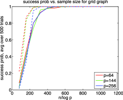
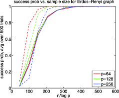
(a) Grid graph	(b) Erdös–Renyi graph
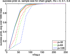
(c) Chain graph

Figure 3: Comparison between $\ell_{1}$-regularized logistic vs. linear regression methods for graph recovery. Each panel plots of the probability of correct graph recovery vs. the rescaled sample size $n/\log p$; solid curves correspond to linear regression (method in this paper), whereas dotted curves correspond to logistic regression RavEtal10 . Curves are based on average performance over 500 trials. (a) Simulation results for two-dimensional grids with $d=4$ neighbors, and number of nodes $p$ varying over $\{64,144,256\}$. Consistent with theory, when plotted vs. the rescaled sample size $n/\log p$, all three curves (red, blue, green) are well aligned with one another. Both linear and logistic regression transition from failure to success at a similar point. (b) Analogous results for an Erdös–Renyi graph with edge probability $3/p$. (c) Analogous results for a chain-structured graph with maximum degree $d=2$.

In Figure 3 we present the results of simulations with two goals: (i) to test the $n\approx\log p$ scaling of the required sample size; and (ii) to compare $\ell_{1}$-regularized nodewise linear regression (Algorithms 3 and 4) to $\ell_{1}$-regularized nodewise logistic regression RavEtal10 . We ran simulations for the two methods on both tree-structured and nontree graphs with data generated from a binary Ising model, with node weights $\theta_{s}=0.1$ and edge weights $\theta_{st}=0.3$. To save on computation, we employed the neighborhood screening method described in Section 4.3 to prune the candidate neighborhood set before performing linear regression. We selected a candidate neighborhood set of size $\lfloor 2.5d\rfloor$ with highest empirical correlations, then performed a single regression against all singleton nodes and products of subsets of the candidate neighborhood set of size at most $d$, via the modified Lasso program (23). The size of the candidate neighborhood set was tuned through repeated runs of the algorithm. For both methods, the optimal choice of regularization parameter $\lambda_{n}$ scales as $\sqrt{\frac{\log p}{n}}$, and we used the same value of $\lambda_{n}$ in comparing logistic to linear regression. In each panel we plot the probability of successful graph recovery versus the rescaled sample size $\frac{n}{\log p}$, with curves of different colors corresponding to graphs (from the same family) of different sizes. Solid lines correspond to linear regression, whereas dotted lines correspond to logistic regression; panels (a), (b) and (c) correspond to grid graphs, Erdös–Renyi random graphs and chain graphs, respectively. For all these graphs, the three solid/dotted curves for different problem sizes are well aligned, showing that the method undergoes a transition from failure to success as a function of the ratio $\frac{n}{\log p}$. In addition, both linear and logistic regression are comparable in terms of statistical efficiency (the number of samples $n$ required for correct graph selection to be achieved).

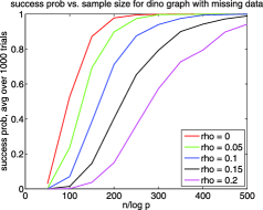
(a) Dino graph with missing data	(b) Chain graph with missing data
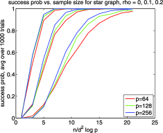
(c) Star graph with missing data, $d\approx\log p$

Figure 4: Simulation results for global and nodewise recovery methods on binary Ising models, allowing for missing data in the observations. Each point represents an average over 1000 trials. Panel (a) shows simulation results for the graphical Lasso method applied to the dinosaur graph with the fraction $\rho$ of missing data varying in $\{0,0.05,0.1,0.15,0.2\}$. Panel (b) shows simulation results for nodewise regression applied to chain graphs for varying $p$ and $\rho$. Panel (c) shows simulation results for nodewise regression applied to star graphs with maximal node degree $d=\log p$ and varying $\rho$.

The main advantage of nodewise linear regression and the graphical Lasso over nodewise logistic regression is that they are straightforward to correct for corrupted or missing data. Figure 4 shows the results of simulations designed to test the behavior of these corrected estimators in the presence of missing data. Panel (a) shows the results of applying the graphical Lasso method, as described in Section 4.1, to the dino graph of Figure 2(e). We again generated data from an Ising model with node weights $0.1$ and edge weights $0.3$. The curves show the probability of success in recovering the 15 edges of the graph, as a function of the rescaled sample size $\frac{n}{\log p}$ for $p=13$. In addition, we performed simulations for different levels of missing data, specified by the parameter $\rho\in\{0,0.05,0.1,0.15,0.2\}$, using the corrected estimator (22). Note that all five runs display a transition from success probability 0 to success probability 1 in roughly the same range, as predicted by our theory. Indeed, since the dinosaur graph has only singleton separators, Corollary 2 ensures that the inverse covariance matrix is exactly graph-structured, so our global recovery method is consistent at the population level. Further note that the curves shift right as the fraction $\rho$ of missing data increases, since the recovery problem becomes incrementally harder.

Panels (b) and (c) of Figure 4 show the results of the nodewise regression method of Section 4.2 applied to chain and star graphs, with increasing numbers of nodes $p\in\{32,64,128\}$ and $p\in\{64,128,256\}$, respectively. For the chain graphs in panel (b), we set node weights of the Ising model equal to $0.1$ and edge weights equal to $0.3$. For the varying-degree star graph in panel (c), we set node weights equal to $0.1$ and edge weights equal to $\frac{1.2}{d}$, where the degree $d$ of the central hub grows with the size of the graph as $\lfloor\log p\rfloor$. Again, we show curves for different levels of missing data, $\rho\in\{0,0.1,0.2\}$. The modified Lasso program (23) was optimized using a form of composite gradient descent due to Agarwal, Negahban and Wainwright AgaEtal11 , guaranteed to converge to a small neighborhood of the optimum even when the problem is nonconvex LohWai11a . In both the chain and star graphs, the three curves corresponding to different problem sizes $p$ at each value of the missing data parameter $\rho$ stack up when plotted against the rescaled sample size. Note that the curves for the star graph stack up nicely with the scaling $\frac{n}{d^{2}\log p}$, rather than the worst-case scaling $n\asymp d^{3}\log p$, corroborating the remark following Proposition 1. Since $d=2$ is fixed for the chain graph, we use the rescaled sample size $\frac{n}{\log p}$ in our plots, as in the plots in Figure 3. Once again, these simulations corroborate our theoretical predictions: the corrected linear regression estimator remains consistent even in the presence of missing data, although the sample size required for consistency grows as the fraction of missing data $\rho$ increases.

5 Discussion

The correspondence between the inverse covariance matrix and graph structure of a Gauss–Markov random field is a classical fact with numerous consequences for estimation of Gaussian graphical models. It has been an open question as to whether similar properties extend to a broader class of graphical models. In this paper, we have provided a partial affirmative answer to this question and developed theoretical results extending such relationships to discrete undirected graphical models.

As shown by our results, the inverse of the ordinary covariance matrix is graph-structured for special subclasses of graphs with singleton separator sets. More generally, we have considered inverses of generalized covariance matrices, formed by introducing indicator functions for larger subsets of variables. When these subsets are chosen to reflect the structure of an underlying junction tree, the edge structure is reflected in the inverse covariance matrix. Our population-level results have a number of statistical consequences for graphical model selection. We have shown that our results may be used to establish consistency (or inconsistency) of standard methods for discrete graph selection, and have proposed new methods for neighborhood recovery which, unlike existing methods, may be applied even when observations are systematically corrupted by mechanisms such as additive noise and missing data. Furthermore, our methods are attractive in their simplicity, in that they only involve simple optimization problems.

References

- (1) {barticle}[mr] \bauthor\bsnmAgarwal, \bfnmAlekh\binitsA., \bauthor\bsnmNegahban, \bfnmSahand\binitsS. and \bauthor\bsnmWainwright, \bfnmMartin J.\binitsM. J. (\byear2012). \btitleFast global convergence of gradient methods for high-dimensional statistical recovery. \bjournalAnn. Statist. \bvolume40 \bpages2452–2482. \biddoi=10.1214/12-AOS1032, issn=0090-5364, mr=3097609 \bptokimsref \endbibitem
- (2) {barticle}[mr] \bauthor\bsnmAnandkumar, \bfnmAnimashree\binitsA., \bauthor\bsnmTan, \bfnmVincent Y. F.\binitsV. Y. F., \bauthor\bsnmHuang, \bfnmFurong\binitsF. and \bauthor\bsnmWillsky, \bfnmAlan S.\binitsA. S. (\byear2012). \btitleHigh-dimensional structure estimation in Ising models: Local separation criterion. \bjournalAnn. Statist. \bvolume40 \bpages1346–1375. \biddoi=10.1214/12-AOS1009, issn=0090-5364, mr=3015028 \bptokimsref \endbibitem
- (3) {barticle}[mr] \bauthor\bsnmBanerjee, \bfnmOnureena\binitsO., \bauthor\bparticleEl \bsnmGhaoui, \bfnmLaurent\binitsL. and \bauthor\bsnmd’Aspremont, \bfnmAlexandre\binitsA. (\byear2008). \btitleModel selection through sparse maximum likelihood estimation for multivariate Gaussian or binary data. \bjournalJ. Mach. Learn. Res. \bvolume9 \bpages485–516. \bidissn=1532-4435, mr=2417243 \bptokimsref \endbibitem
- (4) {bbook}[auto:STB—2013/10/14—10:36:11] \bauthor\bsnmBarndorff-Nielson, \bfnmO. E.\binitsO. E. (\byear1978). \btitleInformation and Exponential Families. \bpublisherWiley, \blocationChichester. \bptokimsref \endbibitem
- (5) {barticle}[mr] \bauthor\bsnmBesag, \bfnmJulian\binitsJ. (\byear1974). \btitleSpatial interaction and the statistical analysis of lattice systems. \bjournalJ. R. Stat. Soc. Ser. B Stat. Methodol. \bvolume36 \bpages192–236. \bidissn=0035-9246, mr=0373208 \bptnotecheck related\bptokimsref \endbibitem
- (6) {bincollection}[mr] \bauthor\bsnmBresler, \bfnmGuy\binitsG., \bauthor\bsnmMossel, \bfnmElchanan\binitsE. and \bauthor\bsnmSly, \bfnmAllan\binitsA. (\byear2008). \btitleReconstruction of Markov random fields from samples: Some observations and algorithms. In \bbooktitleApproximation, Randomization and Combinatorial Optimization. \bpages343–356. \bpublisherSpringer, \blocationBerlin. \biddoi=10.1007/978-3-540-85363-3_28, mr=2538799 \bptokimsref \endbibitem
- (7) {bbook}[mr] \bauthor\bsnmBrown, \bfnmLawrence D.\binitsL. D. (\byear1986). \btitleFundamentals of Statistical Exponential Families. \bpublisherIMS, \blocationHayward, CA. \bidmr=0882001 \bptokimsref \endbibitem
- (8) {barticle}[mr] \bauthor\bsnmCai, \bfnmTony\binitsT., \bauthor\bsnmLiu, \bfnmWeidong\binitsW. and \bauthor\bsnmLuo, \bfnmXi\binitsX. (\byear2011). \btitleA constrained minimization approach to sparse precision matrix estimation. \bjournalJ. Amer. Statist. Assoc. \bvolume106 \bpages594–607. \biddoi=10.1198/jasa.2011.tm10155, issn=0162-1459, mr=2847973 \bptokimsref \endbibitem
- (9) {bbook}[mr] \bauthor\bsnmCarroll, \bfnmR. J.\binitsR. J., \bauthor\bsnmRuppert, \bfnmD.\binitsD. and \bauthor\bsnmStefanski, \bfnmL. A.\binitsL. A. (\byear1995). \btitleMeasurement Error in Nonlinear Models. \bpublisherChapman & Hall, \blocationLondon. \bidmr=1630517 \bptokimsref \endbibitem
- (10) {barticle}[auto:STB—2013/10/14—10:36:11] \bauthor\bsnmChow, \bfnmC. I.\binitsC. I. and \bauthor\bsnmLiu, \bfnmC. N.\binitsC. N. (\byear1968). \btitleApproximating discrete probability distributions with dependence trees. \bjournalIEEE Trans. Inform. Theory \bvolume14 \bpages462–467. \bptokimsref \endbibitem
- (11) {barticle}[mr] \bauthor\bsnmDarroch, \bfnmJ. N.\binitsJ. N. and \bauthor\bsnmSpeed, \bfnmT. P.\binitsT. P. (\byear1983). \btitleAdditive and multiplicative models and interactions. \bjournalAnn. Statist. \bvolume11 \bpages724–738. \biddoi=10.1214/aos/1176346240, issn=0090-5364, mr=0707924 \bptokimsref \endbibitem
- (12) {barticle}[mr] \bauthor\bsnmd’Aspremont, \bfnmAlexandre\binitsA., \bauthor\bsnmBanerjee, \bfnmOnureena\binitsO. and \bauthor\bparticleEl \bsnmGhaoui, \bfnmLaurent\binitsL. (\byear2008). \btitleFirst-order methods for sparse covariance selection. \bjournalSIAM J. Matrix Anal. Appl. \bvolume30 \bpages56–66. \biddoi=10.1137/060670985, issn=0895-4798, mr=2399568 \bptokimsref \endbibitem
- (13) {barticle}[mr] \bauthor\bsnmDempster, \bfnmA. P.\binitsA. P., \bauthor\bsnmLaird, \bfnmN. M.\binitsN. M. and \bauthor\bsnmRubin, \bfnmD. B.\binitsD. B. (\byear1977). \btitleMaximum likelihood from incomplete data via the EM algorithm. \bjournalJ. R. Stat. Soc. Ser. B Stat. Methodol. \bvolume39 \bpages1–38. \bidissn=0035-9246, mr=0501537 \bptnotecheck related\bptokimsref \endbibitem
- (14) {barticle}[auto:STB—2013/10/14—10:36:11] \bauthor\bsnmFriedman, \bfnmJ.\binitsJ., \bauthor\bsnmHastie, \bfnmT.\binitsT. and \bauthor\bsnmTibshirani, \bfnmR.\binitsR. (\byear2008). \btitleSparse inverse covariance estimation with the graphical Lasso. \bjournalBiostatistics \bvolume9 \bpages432–441. \bptokimsref \endbibitem
- (15) {barticle}[mr] \bauthor\bsnmGrimmett, \bfnmG. R.\binitsG. R. (\byear1973). \btitleA theorem about random fields. \bjournalBull. Lond. Math. Soc. \bvolume5 \bpages81–84. \bidissn=0024-6093, mr=0329039 \bptokimsref \endbibitem
- (16) {bbook}[mr] \bauthor\bsnmHorn, \bfnmRoger A.\binitsR. A. and \bauthor\bsnmJohnson, \bfnmCharles R.\binitsC. R. (\byear1990). \btitleMatrix Analysis. \bpublisherCambridge Univ. Press, \blocationCambridge. \bidmr=1084815 \bptokimsref \endbibitem
- (17) {barticle}[mr] \bauthor\bsnmIbrahim, \bfnmJoseph G.\binitsJ. G., \bauthor\bsnmChen, \bfnmMing-Hui\binitsM.-H., \bauthor\bsnmLipsitz, \bfnmStuart R.\binitsS. R. and \bauthor\bsnmHerring, \bfnmAmy H.\binitsA. H. (\byear2005). \btitleMissing-data methods for generalized linear models: A comparative review. \bjournalJ. Amer. Statist. Assoc. \bvolume100 \bpages332–346. \biddoi=10.1198/016214504000001844, issn=0162-1459, mr=2166072 \bptokimsref \endbibitem
- (18) {bincollection}[auto:STB—2013/10/14—10:36:11] \bauthor\bsnmJacob, \bfnmL.\binitsL., \bauthor\bsnmObozinski, \bfnmG.\binitsG. and \bauthor\bsnmVert, \bfnmJ. P.\binitsJ. P. (\byear2009). \btitleGroup Lasso with overlap and graph Lasso. In \bbooktitleInternational Conference on Machine Learning (ICML) \bpages433–440. \bpublisherACM, \blocationNew York. \bptokimsref \endbibitem
- (19) {barticle}[auto:STB—2013/10/14—10:36:11] \bauthor\bsnmJalali, \bfnmA.\binitsA., \bauthor\bsnmRavikumar, \bfnmP. D.\binitsP. D., \bauthor\bsnmVasuki, \bfnmV.\binitsV. and \bauthor\bsnmSanghavi, \bfnmS.\binitsS. (\byear2011). \btitleOn learning discrete graphical models using group-sparse regularization. \bjournalJournal of Machine Learning Research—Proceedings Track \bvolume15 \bpages378–387. \bptokimsref \endbibitem
- (20) {bbook}[mr] \bauthor\bsnmKoller, \bfnmDaphne\binitsD. and \bauthor\bsnmFriedman, \bfnmNir\binitsN. (\byear2009). \btitleProbabilistic Graphical Models: Principles and Techniques. \bpublisherMIT Press, \blocationCambridge. \bidmr=2778120 \bptokimsref \endbibitem
- (21) {bbook}[mr] \bauthor\bsnmLauritzen, \bfnmSteffen L.\binitsS. L. (\byear1996). \btitleGraphical Models. \bpublisherOxford Univ. Press, \blocationNew York. \bidmr=1419991 \bptokimsref \endbibitem
- (22) {barticle}[mr] \bauthor\bsnmLauritzen, \bfnmS. L.\binitsS. L. and \bauthor\bsnmSpiegelhalter, \bfnmD. J.\binitsD. J. (\byear1988). \btitleLocal computations with probabilities on graphical structures and their application to expert systems. \bjournalJ. R. Stat. Soc. Ser. B Stat. Methodol. \bvolume50 \bpages157–224. \bidissn=0035-9246, mr=0964177 \bptokimsref \endbibitem
- (23) {barticle}[mr] \bauthor\bsnmLiu, \bfnmHan\binitsH., \bauthor\bsnmHan, \bfnmFang\binitsF., \bauthor\bsnmYuan, \bfnmMing\binitsM., \bauthor\bsnmLafferty, \bfnmJohn\binitsJ. and \bauthor\bsnmWasserman, \bfnmLarry\binitsL. (\byear2012). \btitleHigh-dimensional semiparametric Gaussian copula graphical models. \bjournalAnn. Statist. \bvolume40 \bpages2293–2326. \biddoi=10.1214/12-AOS1037, issn=0090-5364, mr=3059084 \bptokimsref \endbibitem
- (24) {barticle}[mr] \bauthor\bsnmLiu, \bfnmHan\binitsH., \bauthor\bsnmLafferty, \bfnmJohn\binitsJ. and \bauthor\bsnmWasserman, \bfnmLarry\binitsL. (\byear2009). \btitleThe nonparanormal: Semiparametric estimation of high dimensional undirected graphs. \bjournalJ. Mach. Learn. Res. \bvolume10 \bpages2295–2328. \bidissn=1532-4435, mr=2563983 \bptokimsref \endbibitem
- (25) {barticle}[mr] \bauthor\bsnmLoh, \bfnmPo-Ling\binitsP.-L. and \bauthor\bsnmWainwright, \bfnmMartin J.\binitsM. J. (\byear2012). \btitleHigh-dimensional regression with noisy and missing data: Provable guarantees with nonconvexity. \bjournalAnn. Statist. \bvolume40 \bpages1637–1664. \biddoi=10.1214/12-AOS1018, issn=0090-5364, mr=3015038 \bptokimsref \endbibitem
- (26) {bmisc}[auto:STB—2013/10/14—10:36:11] \bauthor\bsnmLoh, \bfnmP.\binitsP. and \bauthor\bsnmWainwright, \bfnmM. J.\binitsM. J. (\byear2013). \bhowpublishedSupplement to “Structure estimation for discrete graphical models: Generalized covariance matrices and their inverses.” DOI:\doiurl10.1214/13-AOS1162SUPP. \bptokimsref \endbibitem
- (27) {barticle}[mr] \bauthor\bsnmMeinshausen, \bfnmNicolai\binitsN. and \bauthor\bsnmBühlmann, \bfnmPeter\binitsP. (\byear2006). \btitleHigh-dimensional graphs and variable selection with the lasso. \bjournalAnn. Statist. \bvolume34 \bpages1436–1462. \biddoi=10.1214/009053606000000281, issn=0090-5364, mr=2278363 \bptokimsref \endbibitem
- (28) {barticle}[auto:STB—2013/10/14—10:36:11] \bauthor\bsnmNewman, \bfnmM. E. J.\binitsM. E. J. and \bauthor\bsnmWatts, \bfnmD. J.\binitsD. J. (\byear1999). \btitleScaling and percolation in the small-world network model. \bjournalPhys. Rev. E (3) \bvolume60 \bpages7332–7342. \bptokimsref \endbibitem
- (29) {barticle}[mr] \bauthor\bsnmObozinski, \bfnmGuillaume\binitsG., \bauthor\bsnmWainwright, \bfnmMartin J.\binitsM. J. and \bauthor\bsnmJordan, \bfnmMichael I.\binitsM. I. (\byear2011). \btitleSupport union recovery in high-dimensional multivariate regression. \bjournalAnn. Statist. \bvolume39 \bpages1–47. \biddoi=10.1214/09-AOS776, issn=0090-5364, mr=2797839 \bptokimsref \endbibitem
- (30) {barticle}[mr] \bauthor\bsnmRavikumar, \bfnmPradeep\binitsP., \bauthor\bsnmWainwright, \bfnmMartin J.\binitsM. J. and \bauthor\bsnmLafferty, \bfnmJohn D.\binitsJ. D. (\byear2010). \btitleHigh-dimensional Ising model selection using -regularized logistic regression. \bjournalAnn. Statist. \bvolume38 \bpages1287–1319. \biddoi=10.1214/09-AOS691, issn=0090-5364, mr=2662343 \bptokimsref \endbibitem
- (31) {barticle}[mr] \bauthor\bsnmRavikumar, \bfnmPradeep\binitsP., \bauthor\bsnmWainwright, \bfnmMartin J.\binitsM. J., \bauthor\bsnmRaskutti, \bfnmGarvesh\binitsG. and \bauthor\bsnmYu, \bfnmBin\binitsB. (\byear2011). \btitleHigh-dimensional covariance estimation by minimizing -penalized log-determinant divergence. \bjournalElectron. J. Stat. \bvolume5 \bpages935–980. \biddoi=10.1214/11-EJS631, issn=1935-7524, mr=2836766 \bptokimsref \endbibitem
- (32) {bbook}[mr] \bauthor\bsnmRockafellar, \bfnmR. Tyrrell\binitsR. T. (\byear1970). \btitleConvex Analysis. \bpublisherPrinceton Univ. Press, \blocationPrinceton, NJ. \bidmr=0274683 \bptokimsref \endbibitem
- (33) {barticle}[mr] \bauthor\bsnmRothman, \bfnmAdam J.\binitsA. J., \bauthor\bsnmBickel, \bfnmPeter J.\binitsP. J., \bauthor\bsnmLevina, \bfnmElizaveta\binitsE. and \bauthor\bsnmZhu, \bfnmJi\binitsJ. (\byear2008). \btitleSparse permutation invariant covariance estimation. \bjournalElectron. J. Stat. \bvolume2 \bpages494–515. \biddoi=10.1214/08-EJS176, issn=1935-7524, mr=2417391 \bptokimsref \endbibitem
- (34) {bbook}[mr] \bauthor\bsnmRubin, \bfnmDonald B.\binitsD. B. (\byear1987). \btitleMultiple Imputation for Nonresponse in Surveys. \bpublisherWiley, \blocationNew York. \biddoi=10.1002/9780470316696, mr=0899519 \bptokimsref \endbibitem
- (35) {barticle}[mr] \bauthor\bsnmSanthanam, \bfnmNarayana P.\binitsN. P. and \bauthor\bsnmWainwright, \bfnmMartin J.\binitsM. J. (\byear2012). \btitleInformation-theoretic limits of selecting binary graphical models in high dimensions. \bjournalIEEE Trans. Inform. Theory \bvolume58 \bpages4117–4134. \biddoi=10.1109/TIT.2012.2191659, issn=0018-9448, mr=2943079 \bptokimsref \endbibitem
- (36) {barticle}[auto:STB—2013/10/14—10:36:11] \bauthor\bsnmWainwright, \bfnmM. J.\binitsM. J. and \bauthor\bsnmJordan, \bfnmM. I.\binitsM. I. (\byear2008). \btitleGraphical models, exponential families, and variational inference. \bjournalFound. Trends Mach. Learn. \bvolume1 \bpages1–305. \bnoteISSN 1935-8237. \bptokimsref \endbibitem
- (37) {barticle}[mr] \bauthor\bsnmXue, \bfnmLingzhou\binitsL. and \bauthor\bsnmZou, \bfnmHui\binitsH. (\byear2012). \btitleRegularized rank-based estimation of high-dimensional nonparanormal graphical models. \bjournalAnn. Statist. \bvolume40 \bpages2541–2571. \biddoi=10.1214/12-AOS1041, issn=0090-5364, mr=3097612 \bptokimsref \endbibitem
- (38) {barticle}[mr] \bauthor\bsnmYuan, \bfnmMing\binitsM. (\byear2010). \btitleHigh dimensional inverse covariance matrix estimation via linear programming. \bjournalJ. Mach. Learn. Res. \bvolume11 \bpages2261–2286. \bidissn=1532-4435, mr=2719856 \bptokimsref \endbibitem
- (39) {barticle}[mr] \bauthor\bsnmYuan, \bfnmMing\binitsM. and \bauthor\bsnmLin, \bfnmYi\binitsY. (\byear2007). \btitleModel selection and estimation in the Gaussian graphical model. \bjournalBiometrika \bvolume94 \bpages19–35. \biddoi=10.1093/biomet/asm018, issn=0006-3444, mr=2367824 \bptokimsref \endbibitem
- (40) {barticle}[mr] \bauthor\bsnmZhao, \bfnmPeng\binitsP. and \bauthor\bsnmYu, \bfnmBin\binitsB. (\byear2006). \btitleOn model selection consistency of Lasso. \bjournalJ. Mach. Learn. Res. \bvolume7 \bpages2541–2563. \bidissn=1532-4435, mr=2274449 \bptokimsref \endbibitem