PICACS: self-consistent modelling of galaxy cluster scaling relations

Abstract

In this paper, we introduce PICACS, a physically-motivated, internally consistent model of scaling relations between galaxy cluster masses and their observable properties. This model can be used to constrain simultaneously the form, scatter (including its covariance) and evolution of the scaling relations, as well as the masses of the individual clusters. In this framework, scaling relations between observables (such as that between X-ray luminosity and temperature) are modelled explicitly in terms of the fundamental mass-observable scaling relations, and so are fully constrained without being fit directly. We apply the PICACS model to two observational datasets, and show that it performs as well as traditional regression methods for simply measuring individual scaling relation parameters, but reveals additional information on the processes that shape the relations while providing self-consistent mass constraints. Our analysis suggests that the observed combination of slopes of the scaling relations can be described by a deficit of gas in low-mass clusters that is compensated for by elevated gas temperatures, such that the total thermal energy of the gas in a cluster of given mass remains close to self-similar expectations. This is interpreted as the result of AGN feedback removing low entropy gas from low mass systems, while heating the remaining gas. We deconstruct the luminosity-temperature ($LT$) relation and show that its steepening compared to self-similar expectations can be explained solely by this combination of gas depletion and heating in low mass systems, without any additional contribution from a mass dependence of the gas structure. Finally, we demonstrate that a self-consistent analysis of the scaling relations leads to an expectation of self-similar evolution of the $LT$ relation that is significantly weaker than is commonly assumed.

1 Introduction

Simple theoretical arguments lead to an expectation of power-law scaling relations between the masses of galaxy clusters and their observable properties (Kaiser, 1986; Bryan & Norman, 1998). These scaling relations have been the subject of a great deal of attention, in particular those involving X-ray observations of the properties of the intra-cluster medium (ICM) (e.g. Finoguenov, Reiprich & Böhringer, 2001; Reiprich & Böhringer, 2002; Sanderson et al., 2003; Vikhlinin et al., 2003). These X-ray scaling relations are of interest, as correctly modelling the forms of the scaling relations tests our understanding of the physical processes that heat and shape the ICM over cluster lifetimes. Furthermore, if the forms of the scaling relations are known to some precision, then they provide an efficient tool to estimate cluster masses in the absence of detailed data to allow, for instance, an X-ray hydrostatic mass analysis.

When mass estimates are not available for clusters, it is also common to study the correlations between X-ray properties as a way to gain insight into ICM physics. For this reason, the X-ray luminosity-temperature ($LT$) relation has been extensively studied (e.g. Mitchell et al., 1979; Edge & Stewart, 1991; Markevitch, 1998; Pratt et al., 2009; Maughan et al., 2012). It is widely found that the slope of the $LT$ relation is steeper than that expected if gravitational heating of the ICM were the only significant influence (but see Maughan et al., 2012, for a notable exception). Successful models of additional ICM physics are then expected to explain the steepening of the $LT$ relation. In this paper, we will argue that fitting models of the $LT$ relation to observations of clusters and investigating departures from self-similarity is not optimal. A much better approach is to jointly model the scaling relations between cluster observables and their masses, and use those to dictate the form of the $LT$ relation.

The usual approach in these endeavours is to model each of the scaling relations independently using a form of linear regression. Perhaps the most popular form is the BCES method, which accounts for errors in the $x$ and $y$ variables, and intrinsic scatter in the population being modelled (Akritas & Bershady, 1996). More recently, Bayesian techniques have been employed to allow greater flexibility in modelling (Kelly, 2007; Andreon & Hurn, 2010), but these are usually only employed to look at individual scaling relations. Bayesian techniques are now commonly used in cosmological studies, with many of these jointly modelling one or more mass-observable scaling relation (e.g. Rozo et al., 2009; Benson et al., 2011). The most advanced treatment of the X-ray scaling relations thus far is the self-consistent modelling of the scaling relations and mass function for a large sample of clusters by Mantz et al. (2010b, a), which included joint modelling of the mass scaling of $L$ and $T$.

There is far more information in the cluster datasets than is typically used in studies of the scaling relations of cluster populations. In this paper, we present a method of Physically-motivated, Internally Consistent Analysis of Cluster Scaling (PICACS) that jointly constrains the form of the scaling relations between different observables and cluster masses. This maximises the use of the observational data, provides new information on the extent to which different observable properties depart from self-similar behaviour, and gives improved mass estimates for individual clusters.

The paper is laid out as follows. In §2 we derive the set of scaling relations used to model the cluster population, and then present the statistical framework used to implement the model in §3. We then apply the new technique to observed samples of galaxy clusters with individual hydrostatic mass measurements (§4) and without mass estimates (§5). We examine the implications of our results for estimating clusters masses in §6, and for dissecting the traditional $TM$ and $LT$ relations in §7 and §8 respectively. We finish with a discusion of the limitations of the methodology in §9, before summarising our main results and conclusions in §10. Throughout the paper, we assume a $\Lambda$CDM cosmology with $\Omega_{M}=0.3$, $\Omega_{\Lambda}=0.7$ and $H_{0}=70\mathrm{\mbox{$\mathrm{~{}km}$}\mathrm{\mbox{$\mathrm{~{}s}$}^{-1}}\mathrm{\mbox{$\mathrm{~{}Mpc}$}^{-1}}\,}$.

2 Self-Consistent Scaling Relations

The galaxy cluster X-ray scaling relations were proposed by Kaiser (1986), based on simple arguments of self-similarity for clusters dominated by gravity, and their derivations have been extensively covered in the literature (e.g. Bryan & Norman, 1998; Maughan et al., 2006). Here we briefly review the standard derivations of self-similar scaling relations, and then extend them to build a self-consistent set of relations to describe non-self-similar clusters.

The three main properties of the ICM that are observable in X-rays, and are expected to scale with cluster mass, are the temperature ($T$), mass ($\mu$), and luminosity ($L$) of the ICM. We will consider how each of these observables are expected to scale with the total mass ($M$) of a cluster. In order to account for the mass dependence of cluster size, and the evolving background density field from which clusters collapse, it is convenient to consider properties within an overdensity radius $R_{\Delta}$, which encloses a mean density of $\Delta\rho_{c}(z)$. The use of the critical density at the redshift of the cluster as a reference density introduces an expected evolution into the resulting scaling relations, parameterised through

$$E(z)=\sqrt{\Omega_{M}(1+z)^{3}+(1-\Omega_{M}-\Lambda)(1+z)^{2}+\Lambda}$$ (1)

and which describes the redshift dependence of the Hubble parameter. This leads to

$$R_{\Delta} \propto E(z)^{-2/3}M_{\Delta}^{1/3}$$ (2)

which can be used to eliminate $R$ in favour of $M$. In the following derivations, all properties are implicitly measured within the same radius $R_{\Delta}$, and we drop the $\Delta$ subscript for compactness.

2.1 The $\mu M$ Relation

For self-similar clusters, the mass of gas ($\mu$) in the ICM is a constant fraction $f_{\mathrm{gas}}$ of the total mass:

$$\mu =f_{\mathrm{gas}}M$$ (3)

This can be rewritten, with the addition of a slope parameter to allow a mass dependency, as

$$\frac{\mu}{\mu_{0}} =A_{\mu M}\left(\frac{M}{M_{0}}\right)^{B_{\mu M}}$$ (4)

Here $A_{\mu}$ is a constant of proportionality and $\mu_{0}$ and $M_{0}$ are normalisation constants introduced for numerical convenience later. Throughout this work, we use $\mu_{0}=5\times 10^{13}\mathrm{M_{\odot}}$ and $M_{0}=5\times 10^{14}\mathrm{M_{\odot}}$.

We have assumed that the gas fraction is constant with redshift. In principal an evolution term could be included in equation (4), but we defer investigation of the evolution of scaling relations in the PICACS model to a later paper. As an aside, we note that equation (4) is equivalent to writing the mass dependency of $f_{\mathrm{gas}}$ as

$$f_{\mathrm{gas}} =\frac{\mu_{0}}{M_{0}}A_{\mu M}\left(\frac{M}{M_{0}}\right)^{B_{\mu M}-1}$$ (5)

2.2 The $TM$ relation

Assuming that the ICM is in virial equilibrium with the cluster gravitational potential, the virial theorem gives

$$T \propto\frac{M}{R},$$ (6)

Eliminating $R$ yields the well-known, self-similar $TM$ relation:

$$T\propto E(z)^{2/3}M^{2/3}.$$ (7)

which we will generalise to give

$$\frac{T}{T_{0}} =A_{TM}E(z)^{\gamma_{TM}}\left(\frac{M}{M_{0}}\right)^{B_{TM}}$$ (8)

Throughout this work, we use $T_{0}=5\mbox{$\mathrm{~{}keV}$}$.

2.3 The $LM$ Relation

The luminosity of the ICM is dominated by bremsstrahlung emission for $T\gtrsim 2\mbox{$\mathrm{~{}keV}$}$, where line emission is not significant. If we also neglect the weak temperature dependence of the Gaunt factor, then the luminosity is given by

$$L \propto\int\rho_{\mathrm{gas}}^{2}T^{1/2}dV$$ (9)

The integral of the gas density, $\rho_{\mathrm{gas}}$, depends on the distribution of the ICM. We follow Arnaud & Evrard (1999) by factoring the density into a mean density and a dimensionless structural parameter $Q=\left<\rho_{\mathrm{gas}}^{2}\right>/\left<\rho_{\mathrm{gas}}\right>^{2}$ (where angle brackets indicate volume averages), such that equation (9) becomes

$$L \propto E(z)^{2}Qf_{\mathrm{gas}}^{2}T^{1/2}M$$ (10)

In other words, the luminosity of the ICM depends both on the amount of gas in the cluster (via $f_{\mathrm{gas}}$), and how that gas is distributed (via $Q$). For self-similar clusters, $Q$ and $f_{\mathrm{gas}}$ are independent of mass and can be absorbed into the proportionality constant.

It is widespread practice (e.g. Maughan et al., 2006) to derive the self-similar relation between luminosity and mass ($LM$ relation) by setting $Q$ and $f_{\mathrm{gas}}$ to constants and using equation (7) to eliminate $T$ from equation (10). However, this does not maximise the observational information, and if self-similar behaviour breaks down, it becomes unclear which of the mass scalings are being broken.

Instead, we rewrite equation (10) to allow for a power-law mass dependence of the ICM structure parameter $Q$ (moving any constant component into the proportionality constant), giving

$$L \propto E(z)^{2}f_{\mathrm{gas}}^{2}T^{1/2}M^{B_{QM}}$$ (11)

Although we interpret this slope parameter $B_{QM}$ as predominantly describing mass-dependence of $Q$, it could also describe the effects of the increasing contribution of line emission to the luminosity at lower temperatures ($\lesssim 2\mbox{$\mathrm{~{}keV}$}$), which modifies the temperature dependence towards $T^{-1/2}$ in equation (9).

Now, rather than use equation (3) to substitute for $f_{\mathrm{gas}}$, let us instead explicitly keep the observed quantities, and write the bremsstrahlung relation as

$$\frac{L}{L_{0}} =A_{L}E(z)^{\gamma_{L}}\left(\frac{\mu}{\mu_{0}}\right)^{2}\left(\frac{T}{T_{0}}\right)^{1/2}\left(\frac{M}{M_{0}}\right)^{B_{QM}-2}$$ (12)

where $\gamma_{L}=2$ and $B_{QM}=1$ for self-similar clusters, and we set $L_{0}=5\times 10^{44}\mathrm{\mbox{$\mathrm{~{}erg}$}\mathrm{\mbox{$\mathrm{~{}s}$}^{-1}}}$.

The traditional $LM$ relation is then given by substituting equations (4) and (7) to eliminate $\mu$ and $T$ in favour of $M$:

$$\frac{L}{L_{0}} =A_{LM}E(z)^{\gamma_{LM}}\left(\frac{M}{M_{0}}\right)^{B_{LM}}$$ (13)

where

$$A_{LM} =A_{L}A_{\mu M}^{2}A_{TM}^{1/2}$$ (14)

$$B_{LM} =2B_{\mu M}+\frac{1}{2}B_{TM}+B_{QM}-2$$ (15)

$$\gamma_{LM} =\gamma_{L}+\frac{1}{2}\gamma_{TM}$$ (16)

For self-similar clusters in virial equilibrium, $B_{LM}=4/3$ and $\gamma_{LM}=7/3$.

Other, composite, X-ray scaling relations may then be produced by combining the preceding scaling relations, as in the following subsections.

2.4 The $Y_{X}M$ Relation

The product of $\mu$ and $T$ is proportional to the total thermal energy content of the ICM and is usually termed $Y_{X}$, which has been shown to follow a low-scatter correlation with mass (e.g. Kravtsov, Vikhlinin & Nagai, 2006; Maughan, 2007; Arnaud, Pointecouteau & Pratt, 2007, hereafter A07). The $Y_{X}M$ relation is obtained by combining the $\mu M$ and $TM$ relations:

$$\frac{Y_{X}}{Y_{X0}} =A_{YM}E(z)^{\gamma_{YM}}\left(\frac{M}{M_{0}}\right)^{B_{YM}}$$ (17)

where $Y_{X0}=2.5\times 10^{14}\mathrm{M_{\odot}}\mbox{$\mathrm{~{}keV}$}$ and

$$A_{YM} =A_{TM}A_{\mu M}$$ (18)

$$B_{YM} =B_{TM}-B_{\mu M}$$ (19)

$$\gamma_{YM} =\gamma_{TM}$$ (20)

For self-similar clusters in virial equilibrium, $\gamma_{YM}=2/3$ and $B_{YM}=5/3$. A07 argued that the $Y_{X}$ may be the ICM property most closely related to the cluster mass, in which case any deficit of gas in the cluster potential (due to its removal or incomplete accretion) would be balanced by an increase in temperature to leave the total thermal energy unchanged. In this case, a difference in $B_{\mu M}$ from unity would be compensated for by a corresponding change in $B_{TM}$ to maintain $B_{\mu M}+B_{TM}=B_{YM}=5/3$.

2.5 The $LT$ Relation

Finally, the relation between luminosity and temperature ($LT$ relation) has long been used as a key observational diagnostic of non-gravitational processes in clusters, with departures from the self-similar form of the $LT$ relation used to measure the nature and extent of those processes. However, as for the $LM$ relation, the self-similar form of the $LT$ relation is usually derived by substituting equation (7) into equation (10) to eliminate $M$, and then assuming $Q$ and $f_{\mathrm{gas}}$ are constant with mass. This results in an $LT$ relation of the form

$$\frac{L}{L_{0}} =A_{LT}E(z)^{\gamma_{LT}}\left(\frac{T}{T_{0}}\right)^{B_{LT}}$$ (21)

where departures from $\gamma_{LT}=1$ and $B_{LT}=2$ are taken as evidence for similarity breaking. However, this is only true if all of the scaling relations between the cluster observables and mass are self similar. This is made clear if we write the parameters of the $LT$ relation in terms of the PICACS scaling relations:

$$A_{LT} =A_{L}A_{\mu M}^{2}A_{TM}^{1/2-(2B_{\mu M}+B_{TM}/2+B_{QM}-2)/B_{TM}}$$ (22)

$$=A_{LM}A_{TM}^{-B_{LM}/B_{TM}}$$

$$B_{LT} =\frac{2B_{\mu M}+B_{TM}/2+B_{QM}-2}{B_{TM}}$$ (23)

$$=B_{LM}/B_{TM}$$

$$\gamma_{LT} =\gamma_{L}+\gamma_{TM}\left(\frac{1}{2}-\frac{2B_{\mu M}+B_{TM}/2+B_{QM}-2}{B_{TM}}\right)$$ (24)

$$=\gamma_{LM}-\frac{B_{LM}}{B_{TM}}\gamma_{TM}$$

Thus the slope of the $LT$ relation departs from self-similarity if any or all of the slopes of the fundamental scaling relations differ from their self-similar values, but measuring the slope of the $LT$ relation will not tell us which. Similarly, the self-similar evolution of the $LT$ relation differs from $\gamma_{LT}=1$ if the evolution or slopes of the fundamental scaling relations differ from their self-similar values. In other words, a simple measurement of the evolution of the $LT$ relation could imply real evolution, when in fact the fundamental scaling relations evolved self-similarly, but the slope of one or more were not self-similar.

2.6 The PICACS Scaling Relations

Equations (4), (8) and (12) form a physically-motivated, internally consistent description of the fundamental scaling relations between the key X-ray observables and cluster mass. The composite scaling relations in equations (13) and (21) are also well-established, but the explicit dependencies on the fundamental scaling relations are not usually preserved, losing information as a result. We refer to these composite relations, with those dependencies explicitly preserved, as the PICACS scaling relations.

In this paper, We argue that the traditional modelling of the $\mu M$, $LT$, $LM$, and $TM$ relations without recognising their dependencies on the fundamental mass scaling relations is a tool that is at best blunt, but possibly also inaccurate, for the study of cluster scaling relations. Instead we propose the use of the PICACS approach, by which we refer to the joint modelling of cluster populations with the PICACS scaling relations. In the following section we present a statistical framework to enable this modelling.

3 Statistical Framework

Perhaps the most obvious way to measure the PICACS scaling relations would be to fit each relation independently to a sample for which we have observations of $T$, $\mu$, $L$, and an observationally determined $M$ (e.g. from X-ray hydrostatic masses). However, by using Bayesian techniques, it is possible to construct a statistical framework to jointly determine the probability distributions of the PICACS parameters and cluster masses, given the observational data. The following treatment was inspired by the Bayesian analysis of cluster mass-richness relations in Andreon & Hurn (2010).

Generically, Bayes’ theorem can be used express the probability of some model parameters $\theta_{i}$ given observational data $D_{j}$ as

$$P(\theta_{i}|D_{j}) \propto P(D_{j}|\theta_{i})P(\theta_{i})$$ (25)

The probability on the left hand side is referred to as the posterior, while the first term on the right describes the likelihood (${\cal L}$) of the data given the model. The last term describes the prior probabilities of the model parameters.

We can construct the likelihood of the PICACS scaling relations and cluster masses in terms of the observables. The PICACS scaling relations predict the value of each observable given a cluster mass, but observed values are expected to differ from the model predictions due to the intrinsic scatter $\delta_{TM}$, $\delta_{\mu M}$, $\delta_{LM}$ of the population about each relation, and the statistical scatter described by the measurement errors $\sigma_{T}$, $\sigma_{\mu}$, $\sigma_{L}$ on each observed quantity. In the following, we will use the subscripts $obs$ to indicate an observed quantity, $mod$ to indicate a quantity predicted by a PICACS scaling relation, and $int$ to indicate the model prediction including intrinsic scatter.

For example, for a cluster of mass $M$, we might have an observed mass $M_{obs}$ with error $\sigma_{M}$, and a predicted temperature $T_{mod}$ from equation (8). The intrinsic scatter in the relation $\delta_{TM}$ will then randomly shift the temperature to a value $T_{int}$, which we then observe as $T_{obs}$ with error $\sigma_{T}$.

The likelihood of our observation of $M_{obs}$ for a cluster of mass $M$ is simply given by

$${\cal L}_{M} =P(M_{\mathrm{obs}}|M,\sigma_{M})$$ (26)

The likelihood of our observation of $T_{\mathrm{obs}}$ for the same cluster is the product of the probabilities of the cluster being scattered to temperature $T_{\mathrm{int}}$ and then observed at temperature $T_{\mathrm{obs}}$:

$${\cal L}_{T} =P(T_{\mathrm{obs}}|T_{\mathrm{int}},\sigma_{T})P(T_{\mathrm{int}}|T_{\mathrm{mod}},\delta_{TM})$$

$$=P(T_{\mathrm{obs}}|T_{\mathrm{int}},\sigma_{T})P(T_{\mathrm{int}}|M,\theta_{T},\delta_{TM})$$ (27)

where $T_{\mathrm{mod}}$ is the temperature predicted by the $TM$ scaling relation in Equation (8), so is a function of $M$ and the scaling relation parameters $\theta_{T}=(A_{TM},B_{TM},\gamma_{TM})$.

The likelihood of the observation of the gas mass $\mu$ for the same cluster is similarly

$${\cal L}_{\mu} =P(\mu_{\mathrm{obs}}|\mu_{\mathrm{int}},\sigma_{\mu})P(\mu_{\mathrm{int}}|\mu_{\mathrm{mod}},\delta_{\mu M})$$

$$=P(\mu_{\mathrm{obs}}|\mu_{\mathrm{int}},\sigma_{\mu})P(\mu_{\mathrm{int}}|M,\theta_{\mu},\delta_{\mu M})$$ (28)

where $\mu_{\mathrm{mod}}$ is given by equation (4), and is a function of $M$ and the scaling relation parameters $\theta_{\mu}=(A_{\mu M},B_{\mu M})$.

Finally, the likelihood function for $L$ is

$${\cal L}_{L} =P(L_{\mathrm{obs}}|L_{\mathrm{int}},\sigma_{L})P(L_{\mathrm{int}}|L_{mod},\delta_{LM})$$

$$=P(L_{\mathrm{obs}}|L_{\mathrm{int}},\sigma_{L})P(L_{\mathrm{int}}|M,\theta_{L},\delta_{LM})$$ (29)

where $\theta_{L}=(A_{LM},B_{LM},\gamma_{LM})$ are the PICACS $LM$ scaling relation parameters.

3.1 Modelling Covariance

The likelihood expressions derived above assume that the intrinsic scatter and statistical scatter on the observables are all independent The PICACS scaling relations make clear that the intrinsic scatter terms should not be independent. For example, intrinsic scatter in $\mu$ at a given $M$ will contribute to scatter in both the $TM$ and $LM$ relations. Furthermore, the processes driving the intrinsic scatter (e.g. mergers, cooling, AGN feedback) will impact all of the ICM observables to a greater or lesser extent.

The covariance of intrinsic scatter has not been widely studied, but simulations suggest a coherent motion of clusters along the $LT$ relation during mergers (e.g. Rowley, Thomas & Kay, 2004; Hartley et al., 2008), implying correlated scatter in the $TM$ and $LM$ relations. The covariance of several cluster observables has also been investigated in the simulations of Stanek et al. (2010) and Angulo et al. (2012). Observationally, Mantz et al. (2010a) found the correlation of intrinsic scatter in $L$ and $T$ to be consistent with zero, albeit without strong constraints.

The possibility of correlated intrinsic scatter is incorporated into the PICACS model by using a covariance matrix $C_{T\mu L}$ to describe the intrinsic scatter. The diagonal terms are $\delta_{TM}^{2},\delta_{\mu M}^{2},\delta_{LM}^{2}$, while the off-diagonal terms give the covariances between $T_{\mathrm{int}},\mu_{\mathrm{int}}$ and $L_{\mathrm{int}}$. The joint likelihood of the intrinsically scattered values is now

$${\cal L}_{int}=P(T_{\mathrm{int}},\mu_{\mathrm{int}},L_{\mathrm{int}}|M,\theta_{L},\theta_{T},\theta_{\mu},C_{T\mu L})$$ (30)

where the probability distribution is a multivariate Gaussian distribution with mean values given by $(T_{\mathrm{mod}},\mu_{\mathrm{mod}},L_{mod})$ and covariance given by $C_{T\mu L}$. With this change, the full covariance matrix becomes a parameter of the model.

Here we have explicitly assumed that the intrinsic scatter in cluster properties is log-normal in form. This is supported by the results of Maughan (2007), who found that the intrinsic scatter in core-excised luminosities (as used in the present study) is consistent with a log-normal distribution, and Vikhlinin et al. (2009) who found that the intrinsic scatter of core-included luminosities is also consistent with a log-normal distribution. However, it has been found that cool-core related properties of clusters show a bimodal distribution (Sanderson, O’Sullivan & Ponman, 2009), suggesting that a log-normal distribution for the intrinsic scatter of core-included properties is an imperfect (though reasonable) assumption.

Name	z	$T$	$\mu$	$M_{\mathrm{obs}}$	$M_{\mathrm{fit}}$	Reference
		keV	$10^{13}\mathrm{M_{\odot}}$	$10^{14}\mathrm{M_{\odot}}$	$10^{14}\mathrm{M_{\odot}}$
A133	0.0569	$4.02\pm 0.07$	$2.82\pm 0.34$	$3.26\pm 0.39$	$3.06\pm 0.25$	V06
A383	0.1883	$4.67\pm 0.12$	$4.07\pm 0.41$	$3.15\pm 0.32$	$3.42\pm 0.27$	V06
A478	0.0881	$7.70\pm 0.12$	$9.89\pm 1.30$	$7.90\pm 1.04$	$8.19\pm 0.74$	V06
A1413	0.1429	$7.16\pm 0.11$	$8.69\pm 0.87$	$7.79\pm 0.78$	$7.51\pm 0.58$	V06
A1795	0.0622	$5.94\pm 0.05$	$6.73\pm 0.58$	$6.20\pm 0.53$	$5.97\pm 0.40$	V06
A1991	0.0592	$2.53\pm 0.06$	$1.35\pm 0.19$	$1.27\pm 0.17$	$1.37\pm 0.13$	V06
A2029	0.0779	$8.22\pm 0.09$	$10.57\pm 0.98$	$8.24\pm 0.76$	$8.61\pm 0.66$	V06
A2390	0.2302	$8.62\pm 0.17$	$16.25\pm 1.63$	$11.05\pm 1.11$	$10.82\pm 0.89$	V06
MKW4	0.0199	$1.59\pm 0.04$	$0.51\pm 0.07$	$0.79\pm 0.10$	$0.72\pm 0.07$	V06
A1983	0.0442	$2.08\pm 0.09$	$0.64\pm 0.09$	$1.09\pm 0.37$	$0.91\pm 0.13$	A07
MKW9	0.0382	$2.32\pm 0.23$	$0.49\pm 0.05$	$0.88\pm 0.20$	$0.80\pm 0.12$	A07
A2717	0.0498	$2.44\pm 0.06$	$1.02\pm 0.05$	$1.10\pm 0.12$	$1.18\pm 0.10$	A07
A2597	0.0852	$3.50\pm 0.09$	$2.51\pm 0.09$	$2.22\pm 0.22$	$2.34\pm 0.19$	A07
A1068	0.1375	$4.46\pm 0.11$	$3.77\pm 0.10$	$3.87\pm 0.28$	$3.66\pm 0.23$	A07
PKS0745-191	0.1028	$7.61\pm 0.27$	$10.71\pm 0.48$	$7.27\pm 0.75$	$7.75\pm 0.63$	A07
A2204	0.1523	$7.89\pm 0.21$	$10.55\pm 0.40$	$8.39\pm 0.81$	$8.25\pm 0.61$	A07

Table 1: X-ray properties of the VA sample clusters taken from V06 and A07 with the addition of the cluster masses ($M_{\mathrm{fit}}$) determined with PICACS ($M_{\mathrm{obs}}$ are the hydrostatic from the referenced works). The V06 values have been rescaled from $H_{0}=72\mathrm{\mbox{$\mathrm{~{}km}$}\mathrm{\mbox{$\mathrm{~{}s}$}^{-1}}\mathrm{\mbox{$\mathrm{~{}Mpc}$}^{-1}}\,}$ to $H_{0}=70\mathrm{\mbox{$\mathrm{~{}km}$}\mathrm{\mbox{$\mathrm{~{}s}$}^{-1}}\mathrm{\mbox{$\mathrm{~{}Mpc}$}^{-1}}\,}$. Where the uncertainties on the A07 properties were asymmetric, the mean value is used. $T$ values have been rescaled to the $[0.15-1]R_{\mathrm{500}}$ aperture as described in the text. The $T$ and $\mu$ values have not been scaled by the cross calibration factors introduced in the text.

It is also possible to model the effect of covariance in the statistical scatter. This covariance matrices would ideally be known from the analysis of the data, but for the literature data used for the current study, these were not available, and so statistical errors were treated as being independent. In principal it is possible to include the covariance in statistical scatter as additional free parameters in the model, and for completeness we present a strategy for doing so below. However, for the data analysed here, this additional complexity was found to be computationally expensive while making no significant change to the model fits, and was thus neglected.

Describing the statistical scatter with a single covariance matrix is not possible, as the matrix would be different for each cluster due to the differing statistical errors. Instead, the covariance of the statistical scatter can be modelled in terms of the correlation coefficients between the statistical errors on the observed quantities, $r_{T\mu}$, $r_{TL}$, $r_{\mu L}$. The joint likelihood of the observed values of each property would then given by

$${\cal L}_{obs}=P(T_{\mathrm{obs}},\mu_{\mathrm{obs}},L_{\mathrm{obs}}|T_{\mathrm{int}},\mu_{\mathrm{int}},L_{\mathrm{int}},D_{T\mu L})$$ (31)

where the probability distribution is a multivariate Gaussian with mean $T_{\mathrm{int}},\mu_{\mathrm{int}},L_{\mathrm{int}}$ and covariance given by $D_{T\mu L}$, which is defined for each cluster with diagonal elements $\sigma_{T}^{2},\sigma_{\mu}^{2},\sigma_{L}^{2}$, and off-diagonal elements $r_{T\mu}/(\sigma_{T}\sigma_{\mu}),r_{TL}/(\sigma_{T}\sigma_{L}),r_{\mu L}/(\sigma_{\mu}\sigma_{L})$. Here the $\sigma$ terms are different for each cluster (the measurement errors), but the correlation coefficients $r$ are in common. The three correlation coefficients are thus the model parameters describing the covariance of statistical scatter.

Neglecting the covariance in the statistical scatter, the likelihood of the observed values is just

$${\cal L}_{obs}=P(T_{\mathrm{obs}}|T_{\mathrm{int}},\sigma_{T})P(\mu_{\mathrm{obs}}|\mu_{\mathrm{int}},\sigma_{\mu})P(L_{\mathrm{obs}}|L_{\mathrm{int}},\sigma_{L})$$ (32)

3.2 The Final Joint Likelihood

For a set of observations of multiple clusters (denoted by the index $i$), we take the product of each likelihood evaluated over all clusters. The joint likelihood of our observations is then given by

$${\cal L} =\prod_{i}{\cal L}_{M,i}{\cal L}_{int,i}{\cal L}_{obs,i}$$ (33)

The posterior probability distribution of our model parameters is

$$P(\theta_{T},\theta_{\mu},\theta_{L},M,T_{\mathrm{int}},\mu_{\mathrm{int}},L_{\mathrm{int}}|M_{\mathrm{obs}},T_{\mathrm{obs}},\mu_{\mathrm{obs}},L_{\mathrm{obs}})\\ \propto{\cal L}\,P(\theta_{T})P(\theta_{\mu})P(\theta_{L})P(M)P(C_{T\mu L})$$ (34)

Note that the cluster mass $M$ is a parameter of our model, as are the intrinsically scattered quantities. The latter are simply nuisance parameters that are marginalised over, but the appearance of $M$ as a parameter means that the PICACS framework can be used to constrain $M$ given a combination of $M_{\mathrm{obs}}$ and/or priors on the form of some or all of the scaling relations. A key advantage of this method is that all of the observables are being fit against the same cluster mass in an internally consistent manner.

As we will demonstrate later, it is entirely possible to fit the PICACS relations to the observed quantities without an observed mass for the clusters being considered. In this case, we remove ${\cal L}_{M}$ from our likelihood function, but keep $M$ as a parameter of the model. $M$ can then be constrained by the PICACS scaling relations, but care is needed as strong degeneracies arise between the scaling relation parameters and between the intrinsic scatter terms. To avoid this, informative priors are required on a subset of the parameters, as discussed in §5.1.

PICACS shares some features and much of its philosophy with the Mantz et al. (2010a) approach, but is not designed with cosmological analyses in mind, and so currently lacks the ability to model selection biases, which is a major strength of the Mantz et al. (2010a) work. On the other hand, PICACS has a more detailed model of the inter-dependency of the scaling relations (specifically the inclusion of a variable slope in the $\mu M$ relation and the explicit inclusion of $\mu$ in the $TM$ relations, and $T$ and $\mu$ in the $LM$ relation).

3.3 Implementation

In order to obtain constraints on our model parameters, the posterior distribution must be sampled over the large parameter space. There are many tools available for this generic problem, and the PICACS framework could be implemented in many ways. Here we note a few of the specifics of our implementation. PICACS was developed using the R statistical computing environment (R Development Core Team, 2012), and the posterior probability distribution was analysed using the Bayesian inference package Laplace’s Demon within $R$. Laplace’s Demon contains many Markov Chain Monte Carlo (MCMC) algorithms designed to efficiently sample the posterior probability distribution, and the “Adaptive Metropolis-within-Gibbs” algorithm was found to be effective at sampling the PICACS posterior distribution and converging reliably. We refer the reader to the excellent documentation in Laplace’s Demon for details of the algorithm, as well as an introduction to Bayesian inference.

It is computationally advantageous to rewrite the PICACS scaling relations in log space (we used log₁₀ for convenience). Thus each probability distribution in the likelihood functions is implemented as a Gaussian distribution in log₁₀ space. It is also essential to work with the logarithm of all probabilities, due to the small numerical values involved, and hence we sampled the natural logarithm of the posterior probability distribution, and all of the products in the likelihood and posterior expressions become sums. Unless otherwise stated, a flat prior was assumed for all parameters. Three MCMC chains were run in parallel with randomised initial values and the fits were accepted when the three chains had converged (as determined by examination of the sample distributions). The probability distribution of each parameter was computed from the distribution of samples from the chain after removing the start of each chain until the parameter values were stationary, and combining multiple chains. We summarise the posterior probability distribution of each parameter as the mean, plus or minus the standard deviation of each distribution.

The presence of covariance matrices in the model significantly increases the computational load of evaluating the likelihood. This is because each proposed covariance matrix must be tested and rejected if it is not positive definite. This is particularly burdensome for the case of covariance in the statistical scatter, where the proposed correlation coefficients give a different covariance matrix for each cluster, due to the differing measurement errors for each cluster.

In the following sections we apply the PICACS framework to observational samples to demonstrate its applicability and effectiveness in several scenarios.

4 Application to clusters with observed masses

As a first test, we apply the PICACS framework to a set of clusters with precise mass estimates from X-ray hydrostatic analyses, and compare the performance to that of traditional BCES regression fits. For this study we used the samples of Vikhlinin et al. (2006, hereafter V06) and A07. Both samples target relaxed, low-z clusters with high quality data over a reasonably large range in mass, so are well suited to a first test of PICACS. Both samples have published $M_{\mathrm{obs}}$, $T_{\mathrm{obs}}$ and $\mu_{\mathrm{obs}}$ for each cluster, but neither sample has published luminosities available. We thus removed ${\cal L}_{L}$ and $\theta_{L}$ from PICACS, leaving $\theta_{T}$, $\theta_{\mu}$, $C_{T\mu}$ (the covariance between $T_{\mathrm{int}}$ and $\mu_{\mathrm{int}}$), $r_{T\mu}$ (the correlation between statistical scatter in $T$ and $\mu$) and $M$ as the parameters of interest.

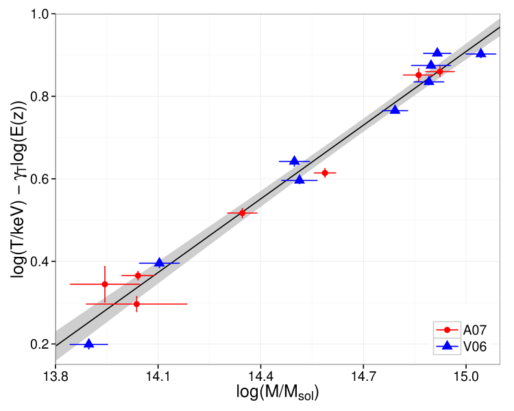
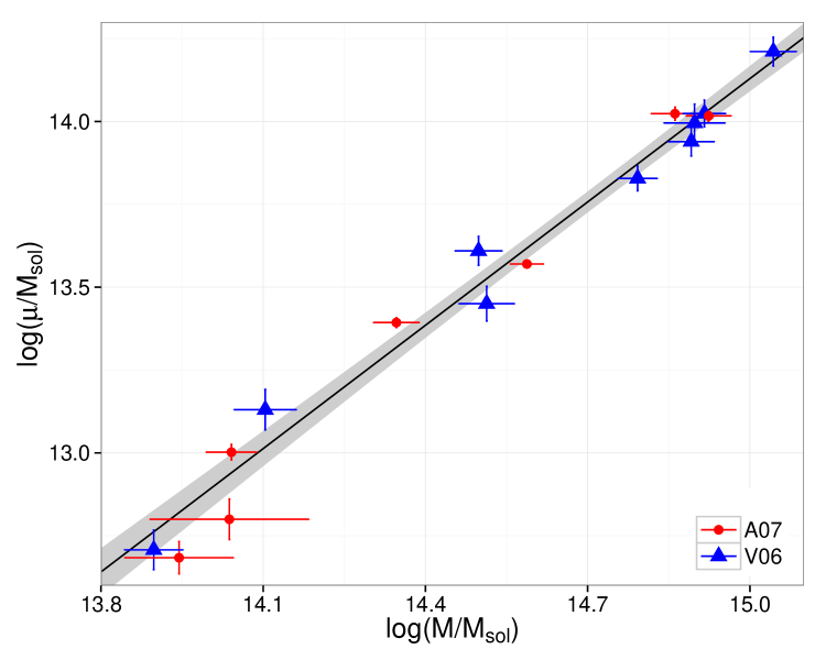
Figure 1: Best fitting PICACS fits to the $TM$ (left) and $\mu M$ (right) scaling relations of the VA sample, with the shaded envelope indicating the $1\sigma$ uncertainty. The A07 clusters have been scaled by the best-fitting $F_{T}$ and $F_{\mu}$ cross-calibration parameters. Note that in these plots, the mass of each cluster is $M_{\mathrm{fit}}$, the mass determined by the combined PICACS fit of the masses and scaling relations.

Method	$A_{TM}$	$B_{TM}$	$\delta_{TM}$	$F_{T}$	$A_{\mu M}$	$B_{\mu M}$	$\delta_{\mu M}$	$F_{\mu}$	$B_{YM}$	$\rho_{T\mu}$
PICACS	$1.07\pm 0.04$	$0.59\pm 0.04$	$0.08\pm 0.03$	$0.97\pm 0.06$	$1.14\pm 0.08$	$1.24\pm 0.07$	$0.14\pm 0.06$	$0.99\pm 0.11$	$1.84\pm 0.10$	$0.3\pm 0.5$
BCES	$1.10\pm 0.02$	$0.60\pm 0.03$	$0.01\pm 0.01$	-	$1.15\pm 0.04$	$1.29\pm 0.05$	$0.02\pm 0.04$	-	-	-

Table 2: Best fitting parameters of the $TM$ and $\mu M$ relations fit to the VA sample using the PICACS and orthogonal BCES methods. For convenience, the intrinsic scatter terms are given in natural log space, so are simply fractional values. For the PICACS fit, the intrinsic scatter values are computed from the diagonal elements of the covariance matrix. $F_{T}$ and $F_{\mu}$ are factors introduced to model relative calibration errors between the instruments used (see text). The final column $\rho_{T\mu}$, gives the Pearson’s correlation for the parameters, derived from the covariance matrix.

The two samples were combined, and duplicate clusters were removed from the A07 sample, and three clusters without measurements at $R_{\mathrm{500}}$ were excluded from the V06 sample. In addition, Abell 907 was removed from the combined list, as it appears in the REXCESS sample (Böhringer et al., 2007), for which we will be using the constraints from this study as independent priors in our subsequent analysis. This gave a combined list of 16 clusters at $0.02<z<0.23$ with a median $z=0.09$, which we refer to as the “VA sample”. The properties of the sample used for this study are summarised in Table 1.

The temperatures from A07 were measured in the $[0.15-0.75]R_{\mathrm{500}}$ aperture so were scaled to the $[0.15-1]R_{\mathrm{500}}$ aperture by multiplying them by $0.955$, the midpoint of the range suggested by A07. Similarly the V06 temperatures were rescaled from the $70\mbox{$\mathrm{~{}kpc}$}-R_{\mathrm{500}}$ aperture in which they were measured, to the $[0.15-1]R_{\mathrm{500}}$ aperture by multiplying them by $0.97$ as recommended in V06. The gas and total masses were all measured within $R_{\mathrm{500}}$.

As the two parent samples were observed with different satellites, Chandra (V06) and XMM-Newton (A07), we introduce additional cross-calibration factors, $F_{T}$ and $F_{\mu}$, such that the A07 $T_{\mathrm{obs}}$ and $\mu_{\mathrm{obs}}$ were multiplied by these factors respectively. We note that the choice to rescale the A07 rather than V06 properties was arbitrary, but as we shall see, these factors turn out to be negligible. The ability to include additional model components such as these scale factors is an advantage of the PICACS approach over BCES regression.

The PICACS models were fit to the VA sample, and the resulting $TM$ and $\mu M$ scaling relations are plotted in Figure 1. The fits were also performed with the standard orthogonal BCES method, and with PICACS assuming independent scatter in the observables. The model parameters obtained with these techniques are summarised in Table 2. In these fits, the evolution parameters $\gamma_{TM}$ and $\gamma_{L}$ were fixed at their self-similar values due to the small redshift range of the sample.

The PICACS fits agree extremely well with the results from the conventional BCES fits (with the exception of the scatter measurements, discussed in the following section), demonstrating that the new technique performs well.

Figure 2: Correlation matrix of the PICACS model parameters for the fit to the VA sample. The posterior densities are shown along the diagonal, with $1\sigma$, $2\sigma$, and $3\sigma$ confidence contours for the pairs of parameters shown on the upper triangle panels. The lower triangle panels show the Pearson’s correlation coefficient for the corresponding pair of parameters (with a text size proportional to the correlation strength). The $\delta$ terms are in natural log space, and were computed from the square root of the diagonal elements of the covariance matrix $C_{T_{\mu}}$ and so do not represent the full information in the covariance matrix.

4.1 Covariance and Degeneracies

Table 2 shows that the measurements of the intrinsic scatter in the $TM$ and $\mu M$ relations differ significantly between the PICACS and BCES methods. However, the definitions of intrinsic scatter also differ, in that the BCES method does not measure scatter itself. Instead, we follow Maughan (2007) in defining the intrinsic scatter as the constant term that must to be added to the combined $T$ (or $\mu$) and $M_{\mathrm{obs}}$ error bars in quadrature in log₁₀ space to produce a reduced $\chi^{2}$ of unity in the $T$ or $\mu$ direction with respect to the BCES regression line. This is not self-consistent, as the best fitting BCES model is not the model which minimises the $\chi^{2}$ in any direction. Furthermore, this approach treats the intrinsic scatter in each relation independently.

In the case of PICACS, if a single scaling relation were fit, then the model masses would move to minimise the scatter in the relation, subject to $M_{\mathrm{obs}}$ and its error. In this case, the scatter measured was found to be consistent with the BCES value. However, when PICACS is jointly fitting $TM$ and $\mu M$ relations, the model masses must satisfy both relations, and could only reduce the scatter significantly below the raw scatter in the data if there were strong positive covariance in the scatter in $T$ and $\mu$. In other words, the model masses from PICACS are not the masses which minimise the scatter in either the $TM$ or $\mu M$ relation alone; they are the masses which jointly satisfy both relations in a consistent way. Using either relation alone would give a lower scatter mass proxy (e.g. for cosmological studies), but would give a different mass for the same cluster. With PICACS we require both relations to give the same mass, which results in larger scatter.

The covariance matrix $C_{T\mu}$ was used to calculate the Pearson’s correlation between $T_{\mathrm{int}}$ and $\mu_{\mathrm{int}}$, giving $\rho_{T\mu}=0.3\pm 0.5$. Thus these data do not provide useful constraints on the correlation of the scatter in these relations. The constraints on the covariance matrix for the intrinsic scatter in the VA sample are summarised in Table 3.

It should be noted that the clusters in the VA sample were selected to be highly relaxed systems to permit reliable hydrostatic masses, so the scatter values measured here and their covariance may not represent the cluster population at large.

	$T_{\mathrm{int}}$	$\mu_{\mathrm{int}}$
$T_{\mathrm{int}}$	$(1.5\pm 1.2)\times 10^{-3}$	$(0.8\pm 1.5)\times 10^{-3}$
$\mu_{\mathrm{int}}$	$(0.8\pm 1.5)\times 10^{-3}$	$(4.5\pm 3.5)\times 10^{-3}$

Table 3: Covariance matrix $C_{T\mu}$ for the PICACS fit to the VA data. The covariance was measured in $\log_{10}$ space.

In addition to the covariance in the intrinsic scatter, we can also investigate the degeneracies in the PICACS model parameters. The correlations between parameters are shown in the scatterplot matrix in Figure 2. This indicates that there is a mild degeneracy between the two normalisation terms and the two slope terms in the model, which is not surprising given the dependency of both scaling relations on the cluster mass. Otherwise, no strong degeneracies exist in the model in this case.

4.2 Mass constraints

The best-fitting masses from the PICACS analysis are given in Table 1, and are compared with $M_{\mathrm{obs}}$ in Figure 3. The agreement is excellent, which should not be surprising, given that $M_{\mathrm{fit}}$ is well-constrained by $M_{\mathrm{obs}}$. It is interesting to note that the uncertainties on $M_{\mathrm{fit}}$ are smaller than those on $M_{\mathrm{obs}}$; the median uncertainty on $M_{\mathrm{obs}}$ is $10\%$, while it is $8\%$ on $M_{\mathrm{fit}}$. This modest increase in precision comes from the additional constraining power given by requiring the best-fit masses to comply with the best-fit scaling relations in addition to being constrained by the error bars on the observed hydrostatic masses.

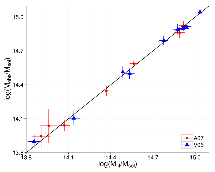
Figure 3: X-ray hydrostatic $M_{\mathrm{obs}}$ is plotted against $M_{\mathrm{fit}}$ from the combined PICACS model for the VA sample. The line shows equality between the two mass estimates.

5 Application to Clusters Without Observed Masses

We now apply the PICACS technique to the REXCESS sample, which is a representative set of low-redshift clusters with high-quality XMM-Newton data (Böhringer et al., 2007). The global X-ray properties ($T$, $L$, and $\mu$) of the clusters were presented in Pratt et al. (2009, hereafter P09) along with a study of the luminosity scaling relations of the sample. X-ray hydrostatic masses are not currently available for the sample. The representative nature of the REXCESS sample, along with the limited redshift range and precisely measured X-ray properties make it a good choice for a second case study of the PICACS methodology. In the following, we use the $T$, $L$, and $\mu$ values of P09, measured out to $R_{\mathrm{500}}$, with the central $15\%$ of $R_{\mathrm{500}}$ excluded for $T$ and $L$. As before, the evolution parameters $\gamma_{TM}$ and $\gamma_{L}$ are fixed at their self-similar values. The properties of the clusters used in this study are summarised in Table 4.

Name	$z$	$T$	$\mu$	$L$	$M_{\mathrm{fit}}$
		keV	$10^{13}\mathrm{M_{\odot}}$	$10^{44}\mathrm{\mbox{$\mathrm{~{}erg}$}\mathrm{\mbox{$\mathrm{~{}s}$}^{-1}}}$	$10^{14}\mathrm{M_{\odot}}$
RXCJ0003$+$0203	0.092	$3.83\pm 0.10$	$1.99\pm 0.04$	$1.15\pm 0.01$	$2.17\pm 0.31$
RXCJ0006$-$3443	0.115	$5.24\pm 0.20$	$4.48\pm 0.11$	$3.17\pm 0.05$	$3.83\pm 0.54$
RXCJ0020$-$2542	0.141	$5.54\pm 0.13$	$4.06\pm 0.06$	$4.05\pm 0.03$	$4.01\pm 0.60$
RXCJ0049$-$2931	0.108	$2.87\pm 0.10$	$1.66\pm 0.03$	$0.99\pm 0.02$	$1.62\pm 0.23$
RXCJ0145$-$5300	0.117	$5.81\pm 0.15$	$4.85\pm 0.06$	$3.87\pm 0.03$	$4.56\pm 0.66$
RXCJ0211$-$4017	0.101	$2.08\pm 0.05$	$0.98\pm 0.01$	$0.48\pm 0.01$	$0.98\pm 0.17$
RXCJ0225$-$2928	0.060	$2.53\pm 0.14$	$0.73\pm 0.02$	$0.31\pm 0.01$	$0.99\pm 0.20$
RXCJ0345$-$4112	0.060	$2.28\pm 0.07$	$0.82\pm 0.02$	$0.37\pm 0.01$	$0.95\pm 0.15$
RXCJ0547$-$3152	0.148	$6.04\pm 0.14$	$5.94\pm 0.04$	$5.73\pm 0.04$	$5.12\pm 0.57$
RXCJ0605$-$3518	0.139	$4.93\pm 0.12$	$4.63\pm 0.05$	$4.23\pm 0.03$	$4.01\pm 0.46$
RXCJ0616$-$4748	0.116	$4.17\pm 0.11$	$2.86\pm 0.04$	$1.88\pm 0.02$	$2.85\pm 0.37$
RXCJ0645$-$5413	0.164	$7.23\pm 0.18$	$10.08\pm 0.11$	$11.33\pm 0.08$	$7.73\pm 0.98$
RXCJ0821$+$0112	0.082	$2.81\pm 0.10$	$1.16\pm 0.03$	$0.54\pm 0.01$	$1.23\pm 0.17$
RXCJ0958$-$1103	0.167	$5.95\pm 0.41$	$4.43\pm 0.20$	$5.21\pm 0.14$	$4.48\pm 0.78$
RXCJ1044$-$0704	0.134	$3.58\pm 0.05$	$3.32\pm 0.04$	$2.99\pm 0.02$	$2.68\pm 0.56$
RXCJ1141$-$1216	0.119	$3.58\pm 0.06$	$2.45\pm 0.02$	$1.69\pm 0.01$	$2.26\pm 0.29$
RXCJ1236$-$3354	0.080	$2.77\pm 0.06$	$1.21\pm 0.02$	$0.61\pm 0.01$	$1.31\pm 0.18$
RXCJ1302$-$0230	0.085	$3.48\pm 0.08$	$1.80\pm 0.02$	$0.83\pm 0.01$	$1.75\pm 0.27$
RXCJ1311$-$0120	0.183	$8.67\pm 0.12$	$10.69\pm 0.06$	$14.93\pm 0.07$	$9.00\pm 1.16$
RXCJ1516$+$0005	0.118	$4.68\pm 0.10$	$3.61\pm 0.04$	$2.76\pm 0.02$	$3.20\pm 0.37$
RXCJ1516$-$0056	0.120	$3.70\pm 0.09$	$2.99\pm 0.04$	$1.77\pm 0.02$	$2.50\pm 0.39$
RXCJ2014$-$2430	0.154	$5.75\pm 0.10$	$7.19\pm 0.07$	$7.47\pm 0.06$	$5.59\pm 0.70$
RXCJ2023$-$2056	0.056	$2.72\pm 0.09$	$1.03\pm 0.02$	$0.40\pm 0.01$	$1.16\pm 0.18$
RXCJ2048$-$1750	0.147	$5.06\pm 0.11$	$5.50\pm 0.05$	$4.40\pm 0.03$	$4.21\pm 0.64$
RXCJ2129$-$5048	0.080	$3.84\pm 0.14$	$2.23\pm 0.04$	$1.19\pm 0.02$	$2.29\pm 0.34$
RXCJ2149$-$3041	0.118	$3.48\pm 0.07$	$2.48\pm 0.03$	$1.58\pm 0.01$	$2.28\pm 0.28$
RXCJ2157$-$0747	0.058	$2.79\pm 0.07$	$1.12\pm 0.02$	$0.37\pm 0.01$	$1.16\pm 0.22$
RXCJ2217$-$3543	0.149	$4.63\pm 0.09$	$4.37\pm 0.04$	$3.69\pm 0.03$	$3.66\pm 0.45$
RXCJ2218$-$3853	0.141	$6.18\pm 0.20$	$5.67\pm 0.07$	$5.55\pm 0.06$	$5.15\pm 0.63$
RXCJ2234$-$3744	0.151	$7.32\pm 0.12$	$9.87\pm 0.10$	$12.28\pm 0.10$	$7.66\pm 0.90$
RXCJ2319$-$7313	0.098	$2.56\pm 0.07$	$1.74\pm 0.03$	$0.97\pm 0.01$	$1.52\pm 0.27$

Table 4: X-ray properties of the REXCESS clusters taken from Pratt et al. (2009) with the addition of the cluster masses determined from the PICACS fits with VA priors. Where the uncertainties on the measured REXCESS properties were asymmetric, the mean value is used. Properties are determined within $R_{\mathrm{500}}$, with the central $0.15R_{\mathrm{500}}$ excluded for $L$ and $T$.

In the absence of $M_{\mathrm{obs}}$ for the REXCESS sample, priors are needed on a subset of the PICACS scaling relation parameters to break the degeneracy between $M_{\mathrm{fit}}$ and the scaling relation shape parameters. Initially, we will maximise the use of the information from the VA sample, and use the constraints on $A_{TM}$, $B_{TM}$, $A_{\mu M}$ and $B_{\mu M}$ from the PICACS analysis summarised in Table 2 (encoded as Gaussian priors in linear space for the $B$ terms and $\log_{10}$ space for the $A$ terms). We also use the posterior probability distribution on the covariance of $T$ and $\mu$ from the VA sample (Table 3) as Gaussian priors on the first $2\times 2$ elements of the full $3\times 3$ $C_{T\mu L}$ covariance matrix. We refer to this set of priors as the “VA priors”. Later (§5.1) we will review the success of the PICACS method with weaker priors. As discussed in §9, the VA priors are not optimal for the REXCESS sample, as the VA sample selected relaxed clusters (necessitated by our use of hydrostatic masses), while the REXCESS clusters encompass the full range of dynamical states.

The best-fitting PICACS relations to the REXCESS sample are plotted in Figure 4, and the parameters are summarised in Table 5. These plots differ from those of conventional scaling relations, as the masses plotted are the best-fitting masses from the combination of scaling relations, and not observed masses. The constraints on the scaling relation parameters are consistent with the VA priors, but with slightly improved precision, and the new constraints on the luminosity scaling parameters are quite precise.

The best-fitting PICACS relations can be compared with the REXCESS $LM$ relation measured in P09. Rescaling to $M_{0}=2\times 10^{14}\mathrm{M_{\odot}}$ and $L_{0}$ of unity as in P09, we find $A_{LM}=(1.08\pm 0.11)\times 10^{44}\mathrm{\mbox{$\mathrm{~{}erg}$}\mathrm{\mbox{$\mathrm{~{}s}$}^{-1}}}$ and $B_{LM}=1.64\pm 0.09$. While the normalisation agrees well with P09, there is mild tension between the values of the slopes ($A_{LM}=(1.08\pm 0.04)\times 10^{44}\mathrm{\mbox{$\mathrm{~{}erg}$}\mathrm{\mbox{$\mathrm{~{}s}$}^{-1}}}$ and $B_{LM}=1.80\pm 0.05$), though we note that the comparison is not exact, as P09 derive their $LM$ relation by using the $Y_{X}M$ relation of A07 to convert their measured $Y_{X}$ values to masses.

Note that $B_{QM}$ is consistent with the self-similar value of 1, which implies no mass scaling of the ICM structural parameter. This is discussed in more detail later in the context of the $LT$ relation. We will now investigate the degeneracies in the model and the sensitivity of the results to the choice of priors.

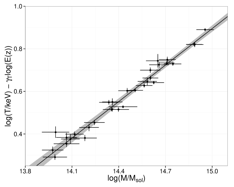
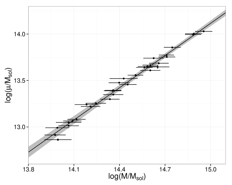
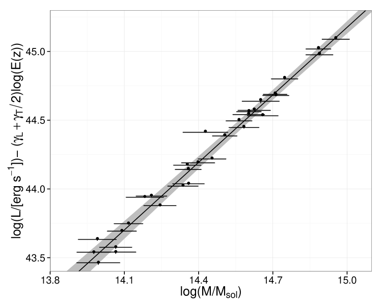
Figure 4: Best fitting $TM$ (left), $\mu M$ (centre), and $LM$ (right) scaling relations for the REXCESS sample, with the shaded envelope indicating the $1\sigma$ uncertainty. The evolution parameters were fixed at their self-similar values, $\gamma_{TM}=2/3,\gamma_{L}=2$. Note that in these plots, the mass of each cluster is $M_{\mathrm{fit}}$, the mass determined by the combined PICACS fit of the masses and scaling relations.

Method	$A_{TM}$	$B_{TM}$	$\delta_{TM}$	$A_{\mu M}$	$B_{\mu M}$	$\delta_{\mu M}$	$A_{LM}$	$B_{LM}$	$\delta_{LM}$	$B_{QM}$
priors	$1.07\pm 0.04$	$0.59\pm 0.04$	$C_{T\mu}$	$1.14\pm 0.08$	$1.24\pm 0.07$	$C_{T\mu}$	-	-	-	-
fit	$1.06\pm 0.03$	$0.57\pm 0.03$	$0.09\pm 0.03$	$1.17\pm 0.06$	$1.16\pm 0.06$	$0.18\pm 0.05$	$0.97\pm 0.08$	$1.64\pm 0.09$	$0.27\pm 0.08$	$1.04\pm 0.06$

Table 5: Best fitting parameters of the PICACS scaling relations fit to the REXCESS sample. All priors were encoded as Gaussian distributions with the specified mean and standard deviation, though the priors on the $A$ terms, while reported in linear space, were implemented as Gaussians in $\log_{10}$ space. For convenience, the intrinsic scatter terms are computed from the diagonal elements of of the covariance matrix in natural log space, so represent fractional scatter.

	$T_{\mathrm{int}}$	$\mu_{\mathrm{int}}$	$L_{\mathrm{int}}$
$T_{\mathrm{int}}$	$(1.8\pm 1.1)\times 10^{-3}$	$(1.1\pm 1.1)\times 10^{-3}$	$(2.1\pm 2.0)\times 10^{-3}$
$\mu_{\mathrm{int}}$	$(1.1\pm 1.1)\times 10^{-3}$	$(6.6\pm 3.6)\times 10^{-3}$	$(8.7\pm 5.3)\times 10^{-3}$
$L_{\mathrm{int}}$	$(2.1\pm 2.0)\times 10^{-3}$	$(8.7\pm 5.3)\times 10^{-3}$	$(1.5\pm 0.9)\times 10^{-2}$
	$\rho_{T\mu}$	$\rho_{TL}$	$\rho_{\mu L}$
	$0.31\pm 0.30$	$0.37\pm 0.31$	$0.85\pm 0.14$

Table 6: Covariance matrix $C_{T\mu L}$ (upper section), and corresponding correlation coefficients (lower section) for the PICACS fit to the REXCESS data. The off-diagonal $Q$ terms were fixed at zero. The covariance was measured in $\log_{10}$ space.

5.1 Covariance and Degeneracies

The intrinsic scatter covariance matrix $C_{T\mu L}$ from our reference fit to the REXCESS data is summarised in Table 6, along with the corresponding correlation coefficients. The data show weak evidence for moderate positive correlation between the scatter in $T$ and $\mu$, and between the scatter in $T$ and $L$. There is strong evidence for a strong positive correlation in the scatter in $\mu$ and $L$. This is not surprising given the strong dependency of $L$ on $\mu$, as illustrated in equation (12). This is comparable to the correlation between $f_{\mathrm{gas}}$ and $L$ of $0.76$ found in the simulations of Stanek et al. (2010). This strong correlation demonstrates that the scatter in the $LM$ relation has a significant contribution from the scatter in the $\mu M$ relation. A measurement of the covariance between observables is important, as it provides a means to model the propagation of biases due to X-ray flux based selection to other observables. For example, our results suggest that without taking this covariance into account, cluster masses estimated from $\mu$ (or indeed $Y_{X}$) in an X-ray flux-limited sample would be biased high, with implications for cosmological studies using such techniques (Nord et al., 2008; Stanek et al., 2010; Angulo et al., 2012).

Figure 5: Correlation matrix of the PICACS model parameters for the fit to the REXCESS sample VA priors. The posterior densities are shown along the diagonal, with $1\sigma$, $2\sigma$, and $3\sigma$ confidence contours for the pairs of parameters shown on the upper triangle panels. The lower triangle panels show the magnitude of the Pearson’s correlation coefficient for the corresponding pair of parameters (with a text size proportional to the correlation strength). The $\delta$ terms are in natural log space, and were computed from the square root of the diagonal elements of the covariance matrix $C_{T\mu L}$ and so do not represent the full information in the covariance matrix.

In Figure 5 the correlations of the model parameters for the reference fit to the REXCESS data are plotted. Unsurprisingly, strong degeneracies exist between the normalisations and between the slopes of the scaling relations. This is due to the mass of each cluster being a free parameter in each scaling relation. We also see that a degeneracy is present between the magnitudes of the scatter, $\delta_{\mu M}$ and $\delta_{LM}$. As above, this is due to the strong dependency of the observed luminosity on the baryon fraction, which is only partially broken by the VA prior on the $T$ and $\mu$ terms of the $C_{T\mu L}$ covariance matrix. Without additional information (e.g. from $M_{\mathrm{obs}}$) it is not possible to constrain $\delta_{\mu M}$ and $\delta_{LM}$ independently.

We investigated the sensitivity of the PICACS approach to the number of priors by removing the VA priors on the $TM$ relation, but keeping those on the $\mu M$ relation, and on the $T,\mu$ components of $C_{T\mu L}$. In this case, the degeneracies between the slope parameters seen in Figure 5 were stronger, and the fit did not become formally stationary, with the slope parameters moving coherently around on these lines of degeneracy. However, various samples taken from the chain showed that all parameters remained within $\approx 1\sigma$ of their values when the full VA priors were used. We thus recommend that priors on two of the three relations are used for analyses where $M_{\mathrm{obs}}$ are not available for at least some of the clusters.

6 PICACS Mass Estimates

A useful application of PICACS is the estimation of masses for clusters without $M_{\mathrm{obs}}$. The best fitting masses are automatically estimated as part of the Bayesian inference process, and provide masses that are fully consistent with the observed properties and derived scaling relations. In §4, we saw that PICACS made a modest improvement to the precision of the hydrostatic mass estimates for the VA sample. In this section we evaluate the performance of PICACS at constraining the unknown masses of the REXCESS sample. The best-fitting PICACS masses from our fits with VA priors are given in Table 4, and the median precision is $14\%$.

The conventional way to estimate X-ray masses for a sample of clusters such as this, in the absence of hydrostatic masses, is to use a single scaling relation to estimate the mass from a single observable (e.g. $T$, $\mu$), simple combinations of observables such as $Y_{X}$ or more generalised combinations of observables (Ettori et al., 2012). Typically, when doing this, only the statistical errors on the observable are propagated to the mass estimate ($M_{\mathrm{fit}}$), or at best, the uncertainties on the shape parameters of the scaling relation are also propagated. Generally, the contribution from the intrinsic scatter in the relation is ignored, but this may be a significant contributor when the statistical errors on the observable are small (e.g. for the REXCESS sample, the median statistical error on $\mu$ is $1\%$). It is straightforward, using a Bayesian approach to include the intrinsic scatter and all of the uncertainties on the final mass estimate.

Let us define a generic scaling relation between mass and some observable (or combination of observables) $X$. Using our previous notation, we have

$$\frac{X}{X_{0}} =A_{X}E(z)^{\gamma_{X}}\left(\frac{M}{M_{0}}\right)^{B_{X}}$$ (35)

and our likelihood function is

$${\cal L}_{X} =P(X_{\mathrm{obs}}|X_{\mathrm{int}},\sigma_{X})P(X_{\mathrm{int}}|X_{\mathrm{mod}},\delta_{X})$$ (36)

$$=P(X_{\mathrm{obs}}|X_{\mathrm{int}},\sigma_{X})P(X_{\mathrm{int}}|M,\theta_{X},\delta_{X})$$ (37)

The posterior probability distribution of the model parameters is then

$$P(\theta_{X},M,X_{\mathrm{int}}|X_{\mathrm{obs}}) \propto{\cal L}_{X}P(\theta_{X})P(M)P(X_{\mathrm{int}})$$ (38)

The priors on $\theta_{X}$ (denoting $A_{X},B_{X},\gamma_{X}$) and $\delta_{X}$ are taken from the scaling relation to be applied. In most cases, $\gamma_{X}$ will be fixed (i.e. at a self-similar value) and $\delta_{X}$ may not have measurement errors, though neither of these factors are limitations of the Bayesian approach. In equation (38), we do not expect significant additional constraints to be placed on $P(\theta_{X}|X_{\mathrm{obs}})$ or $P(X_{\mathrm{int}}|X_{\mathrm{obs}})$, but $P(M)$ will be jointly constrained by the priors on those terms and by $X_{\mathrm{obs}}$, and fully marginalised over all of the uncertainties.

We apply this method to compare the precision of the PICACS mass estimates for the REXCESS sample with those obtained from a single scaling relation. We use the $Y_{X}M$ relation of A07, for which the intrinsic scatter was given as $0.039$ in log₁₀ space, with no uncertainties provided. We convert this to the intrinsic scatter in $Y_{X}$ by dividing by the slope of the A07 $Y_{X}M$ relation, and transform to natural log space to give $\delta_{Y_{X}}=0.16$. Including this intrinsic scatter, and the errors on $A_{Y_{X}}$, $B_{Y_{X}}$ and $Y_{X}$, we find a median uncertainty on the REXCESS masses of $10\%$. Neglecting the intrinsic scatter results in a median mass precision of $4\%$, while including an uncertainty on $\delta_{Y_{X}}$ of the form $\delta_{Y_{X}}=0.16\pm 0.05$ (a reasonable estimate based on our fits to the VA data) slightly increases the median uncertainty to $11\%$. Recall that the median PICACS mass uncertainty for the same clusters was $14\%$. We thus find that in the absence of $M_{\mathrm{obs}}$, PICACS provides mass estimates of slightly poorer precision compared to a single scaling relation, but has the advantage of providing masses that are simultaneously consistent with all of the observables.

As discussed in §4.1, the intrinsic scatter measured with PICACS is typically larger than that measured for single scaling relations with traditional fitting techniques. Thus single or composite scaling relations that are optimised to reduce the intrinsic scatter (such as $Y_{X}$, or the generalised scaling relations of Ettori et al., 2012; Ettori, 2013) may provide higher precision mass estimates. However, such techniques are less useful than PICACS for studying the astrophysics that shape the scaling relations.

7 The PICACS $Y_{X}M$ Relation

The constraints provided by the PICACS model on the $Y_{X}M$ relation are illustrated in Figure 6 shows the posterior probability contours from the VA and REXCESS fits in the $B_{\mu M}-B_{TM}$ plane, along with the line corresponding to the self-similar $Y_{X}M$ relation ($B_{TM}+B_{\mu M}=5/3$). Both fits to the fundamental $TM$ and $\mu M$ relations are inconsistent with self-similarity, but are close to the locus of the self-similar $Y_{X}M$ relation (though recall that the fits are not independent - the VA fit provided the priors for the REXCESS fit).

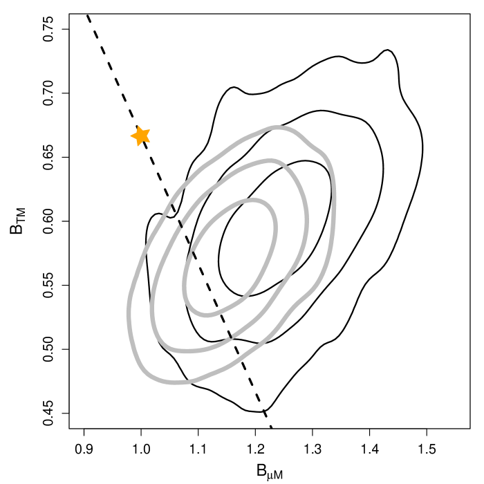
Figure 6: Posterior probability contours for $B_{\mu M}$ and $B_{TM}$ for the fit to the VA data (narrow black contours) and the fit to the REXCESS data with VA priors (thick grey contours). Contours are set at the $1\sigma$, $2\sigma$ and $3\sigma$ levels. The dashed line shows the locus of the self-similar $Y_{X}M$ relation ($B_{\mu M}+B_{TM}=5/3$), and the star marks the self-similar values of $B_{\mu M}=1$, $B_{TM}=2/3$.

This is consistent with the suggestion of A07 that the thermal energy content of the ICM, as represented by $Y_{X}$, is the quantity most closely related to the cluster mass. The low scatter observed in the $Y_{X}M$ relation (Kravtsov, Vikhlinin & Nagai, 2006; Maughan, 2007, A07) implies that the ICM in clusters of a given mass has very similar total thermal energy. Meanwhile, the coordination of the slopes of the $\mu M$ and $TM$ relations to maintain a close to self-similar slope of the $Y_{X}M$ relation while being far from self-similar themselves, implies that the mechanism responsible for depletion (or preventing accretion) of the ICM in lower mass clusters also results in an increased temperature of the remaining gas.

This is compatible with models in which feedback preferentially removes low-entropy gas from the ICM (by removal, we mean that the gas is moved out beyond, or prevented from accreting within, $R_{\mathrm{500}}$), and does so more effectively in low mass systems (e.g. Voit & Donahue, 2005; McNamara & Nulsen, 2007; Pratt et al., 2010; McCarthy et al., 2011). The generic result of this feedback is increasing depletion of the ICM within $R_{\mathrm{500}}$ in lower mas halos, with the remaining higher entropy gas having a temperature consistent with the virial temperature, due to its longer cooling time. However, this does not complete the picture, as a steeper than self-similar $TM$ relation combined with a self-similar $Y_{X}M$ relation would require that the remaining gas is heated by an amount equivalent to the thermal energy lost by the low entropy gas as it cooled and was removed. Furthermore, this heating must affect the mean temperature of the gas outside the central regions ($0.15R_{\mathrm{500}}$), which were excluded in the temperatures used for this study.

These results should be treated with some caution, though, as the VA data alone are agnostic as to whether it is the $TM$ or $Y_{X}M$ relation that is self-similar. It is only when the REXCESS data are analysed with VA priors that the self-similar $Y_{X}M$ relation is strongly preferred, but as discussed in §9, the VA priors are not optimal for the REXCESS sample. In particular, the representative nature of the REXCESS sample means that it will encompass a broader range of feedback states than the relaxed clusters in the VA sample. The most robust results will come from the analysis of representative samples with direct observational constraints on the total masses.

There is some variation in the literature in recent studies of the slopes of these relations. For example, A07 find a shallower $TM$ and steeper $Y_{X}M$ relative to the self-similar values (their best fitting values are very close to our fit to the combined VA data), while Vikhlinin et al. (2009) find slopes of both relations that are consistent with being self-similar. However, the results agree at the $1\sigma$ level, and we argue that a combined analysis of the $TM$ and $\mu M$ relations as presented here is the most useful way to investigate the physical processes shaping these relations.

8 The PICACS $LT$ Relation

We will now examine the $LT$ relation predicted by the PICACS fit to the REXCESS data. Recall that we do not fit the data directly in the $LT$ plane, but the form of the $LT$ relation is given by the self-consistent PICACS models (see equations (22), (23), (24)). In Figure 7 we plot the REXCESS data in the $LT$ plane, along with the PICACS $LT$ relation. Also plotted is the BCES orthogonal regression fit to the data in the $LT$ plane. The REXCESS luminosities were scaled by PICACS evolution parameter $\gamma_{LT}$ for the plot, and this is included in the BCES fit (it is automatically part of the PICACS fit). Note that in the current study, $\gamma_{LT}$ is not fit to any redshift-dependence of the observed cluster properties, but gives the expected self-similar evolution of the $LT$ relation when the dependency on the slopes of the mass observable scaling relations in equation (24) is included. The agreement between the PICACS $LT$ relation and the BCES fit is excellent; the parameters of the $LT$ models are summarised in Table 7.

Figure 7: The $LT$ relation predicted by the PICACS fit to the REXCESS mass scaling relations is plotted with the observed REXCESS properties. The solid line shows the PICACS model, which is not fit directly to the data in this $LT$ plane, with the grey envelope giving the $1\sigma$ uncertainty. The dashed line shows the BCES orthogonal regression as fit to the data in this plot. Luminosities are scaled by the best fitting PICACS $\gamma_{LT}$ evolution parameter (see text for details), and $L$ and $T$ were measured in the $[0.15-1]R_{\mathrm{500}}$ aperture.

Method	$A_{LT}$	$B_{LT}$	$\gamma_{LT}$
PICACS	$0.82\pm 0.05$	$2.87\pm 0.13$	$0.42\pm 0.09$
BCES	$0.84\pm 0.05$	$2.97\pm 0.16$	$0.42^{\dagger}$

Table 7: Best fitting parameters of the $LT$ relation of the REXCESS sample predicted by the PICACS fit and determined from a BCES orthogonal regression to the $LT$ data. The evolution parameter $\gamma_{LT}$ does not include any redshift-dependence of the cluster properties, but gives the self-similar evolution including the dependency on the slopes of the mass observable scaling relations in equation (24). ^†The luminosities were scaled by this fixed value for the BCES fit. See the text for a full discussion of the evolution parameter.

As implied by the agreement with the BCES fit, the PICACS LT relation is also consistent with the P09 fit to the same REXCESS data. The P09 slope of $2.94\pm 0.15$ agrees very well with the PICACS slope in table 7. Rescaling to $L_{0}$ of unity, as in P09, the PICACS normalisation at $5\mbox{$\mathrm{~{}keV}$}$ is $A_{LT}=(4.11\pm 0.26)\times 10^{44}\mathrm{\mbox{$\mathrm{~{}erg}$}\mathrm{\mbox{$\mathrm{~{}s}$}^{-1}}}$, compared with $A_{LT}=(4.06\pm 0.22)\times 10^{44}\mathrm{\mbox{$\mathrm{~{}erg}$}\mathrm{\mbox{$\mathrm{~{}s}$}^{-1}}}$ in P09, also in excellent agreement. Note that the comparison is not exact, as the PICACS fit incorporates correctly the self-similar evolution implied by the slopes of the scaling relations, while in P09 the luminosities are scaled by the traditional self-similar $E(z)^{-1}$. In practice, for this low redshift sample, the differing evolution corrections are negligible.

In fact, while it is reassuring that the PICACS method is able to reproduce the observed $LT$ relation, this should not surprise us; it simply demonstrates that the three PICACS scaling relations form an internally consistent description of the observed properties. Note that the good agreement with the observed $LT$ relation does not necessarily indicate that the individual scaling relations are a good description of the clusters. For instance, if no prior is included on the slope of any of the scaling relations, the degeneracy of the slopes leads to unphysical values for $M_{\mathrm{fit}}$ and the slope parameters. However the internally-consistent scaling relations means that the combination of $A$ and $B$ parameters remains such that the observed $LT$ relations is still reproduced reasonably well. In other words, in the PICACS framework, the observed form of the $LT$ relation is a necessary consequence of requiring the observables to be related to the same masses through power law relations, but is not sensitive to the form of those relations.

8.1 The slope of the $LT$ relation

The advantage of the PICACS method is that while the BCES fit simply tells us that the slope of the $LT$ relation is steeper than the self-similar expectation of $B_{LT}=2$, PICACS enables us to decompose this into the separate mass scaling relations. Table 5 shows that $B_{QM}$ is consistent with unity. Recall that this parameter describes the additional steepening of the luminosity mass relation, beyond that due to the mass dependency of $T$ and $\mu$, which we ascribe predominantly to trends in the ICM structure with mass. The PICACS results thus show that (given the VA priors) the steep slope of the REXCESS $LT$ relation is consistent with the departures from self similarity in $T$ and $\mu$ alone, with no additional contribution from $Q$. This indicates that the ICM structure parameter $Q$ has no mass dependency. While previous work has shown a significant mass dependence of the shape of ICM surface brightness or density profiles (e.g. Sanderson et al., 2003; Croston et al., 2008; Maughan et al., 2012), the dominant effect of those structural trends, when considering a relatively large region such as $R_{\mathrm{500}}$, is reflected by the mass-dependence of $f_{\mathrm{gas}}$. Our results imply that any additional contribution from a mass dependence of $Q$ is not significant. A similar conclusion on the lack of mass dependency of $Q$ was reached by P09, who estimated $Q$ directly from the REXCESS gas density profiles.

Figure 8: Posterior probability contours for $B_{\mu M}$ and $B_{QM}$ for the REXCESS fit with VA priors. Contours are set at the $1\sigma$, $2\sigma$ and $3\sigma$ levels and the dotted lines shows the self-similar values of $B_{\mu M}=1$, $B_{QM}=1$.

This suggests that the $LT$ (and $LM$) relation is predominantly shaped by the same process of gas removal and heating that shaped the $TM$ and $\mu M$ relations. The changes to the $TM$ and $\mu M$ relations act in the sense of steepening the $LT$ relation such that there is no need for additional influence from the $Q$ parameter. This conclusion should, however, be treated with a little caution due to the model degeneracies. Figure 8 shows the confidence contours from the PICACS fit in the $B_{\mu M},B_{QM}$ plane; taking the parameter degeneracy into account, the data can only exclude $B_{\mu M}=1$ at the $\sim 2\sigma$ level. Furthermore, as we have seen, the breaking of the degeneracy between $B_{\mu M}$ and $B_{QM}$ is sensitive to the choice of prior.

8.2 The Evolution of the $LT$ relation

The standard approach to testing evolution of the $LT$ relation is to use equation (21) and define $\gamma_{LT}=1$ as the reference point for self-similar evolution (e.g. Maughan et al., 2006). However, this only holds true if the slopes of all of the mass scaling relations of $T$, $\mu$ and $L$ are self-similar. In the event that they are not, which has been suggested by many observational studies, then the expected self-similar evolution of the $LT$ relation is not $\gamma_{LT}=1$ but is given by equation (24). Of course, this does not imply that the slopes of the scaling relations influence the evolution of clusters, it is simply a consequence of algebraic manipulations used to derive the $LT$ relation.

If applied to a sample covering a significant redshift baseline, PICACS can be used to fit the evolution of all scaling relations self-consistently with their slopes, providing a true measurement of their evolution. We reserve this investigation for a future paper, as measuring the evolution of the scaling relations also requires modelling of sample selection functions to avoid biases masking or mimicking real evolution. This is quite possible within the PICACS framework, along the lines laid out by Mantz et al. (2010b).

For the current study, we simply note that the PICACS fit to the REXCESS data gives the self-similar evolution of the $LT$ relation as $\gamma_{LT}=0.42\pm 0.09$, significantly weaker than the naive expectation of $\gamma_{LT}=1$. Note again that the evolution parameters of the scaling relations were fixed at their self-similar values ($\gamma_{TM}=2/3,\gamma_{L}=2$ and no $f_{\mathrm{gas}}$ evolution); our measurement of $\gamma_{LT}=0.42\pm 0.09$ is not a measurement of the evolution in the REXCESS data, it is a revised prediction of the self-similar evolution due to the non-self-similar slopes of the REXCESS scaling relations. This should be taken into account when establishing a reference self-similar evolution against which to measure deviations. For example, using this PICACS reference for the self-similar $LT$ evolution reduces the significance of the weaker than self-similar (or negative) evolution measured by recent studies (Reichert et al., 2011; Hilton et al., 2012). Those results remain statistically significant compared to our weaker self-similar reference, but the most robust measurements of the evolution will come from a full PICACS analysis of the cluster population to high redshift.

9 Cautions and Caveats

As is clear from Figure 5, strong degeneracies exist in the PICACS model when there are not direct observational constraints on the cluster masses. Not shown in the correlation matrix are the degeneracies between the scaling relation parameters and the fitted cluster masses. These are mitigated with the use of priors on the scaling relations, but without any informative priors, the degeneracy is total; it would be quite possible for masses to fit to unphysical values, and for the normalisations and slopes and scatters of the relations to adjust to compensate. Without $M_{\mathrm{obs}}$ for at least a subset of clusters, the PICACS fits are highly dependent on the choice of priors for a subset of the scaling relation shape parameters.

In the case of our analysis of the REXCESS sample, the VA priors were derived from a sample of relaxed clusters, while the REXCESS clusters encompass a representative range of dynamical states. This difference is unavoidable if X-ray hydrostatic masses are to be used as $M_{\mathrm{obs}}$, but could give rise to systematic effects in the derived REXCESS scaling relations and e.g. our conclusions on the relative contributions of the mass scaling relations to the steepening of the $LT$ relation. The most robust PICACS analysis of representative samples like REXCESS would require mass constraints from a techniques such as gravitational lensing or caustic analyses which are insensitive to cluster dynamical state.

A related complication is the dependence of the observed hydrostatic mass on $T$ and $\rho_{\mathrm{gas}}$. This introduces covariance between $M_{\mathrm{obs}}$ with respect to the true mass and the other X-ray observables. This is not addressed in our model, and so will influence our estimate of the covariance in the VA sample, where we are effectively assuming no intrinsic scatter between the hydrostatic $M_{\mathrm{obs}}$ and the true mass. Furthermore, our analysis also assumed that the log-normal intrinsic scatter covariance matrix was constant as a function of cluster mass. This may well not be the case, as it is clear that non-gravitational processes have an increasing effect on the gas properties of lower mass systems. These issues are also best addressed by using mass estimates that are independent of the X-ray data.

The determination of the covariance in the intrinsic scatter in the cluster population depends crucially on the size of the uncertainties on $L$, $T$, $\mu$ and $M_{\mathrm{obs}}$. The errors on these quantities are generally quoted as statistical errors only, but in fact there may be significant systematic uncertainties on those quantities too. For example, there remain calibration uncertainties for both Chandra and XMM-Newton affecting all measured X-ray properties, and choices made during the reduction and analysis of the data (e.g. data cleaning, background treatment) also contribute. Hydrostatic masses can be influenced by the method used for modelling the density and temperature profiles, and whether a parametric form is assumed for the mass profile (see e.g. the appendix of V06). In the analysis of the VA sample, we allowed for systematic calibration offsets between $T$ and $\mu$ measured with Chandra and XMM-Newton with a simple multiplicative factor, which turned out to be negligible. However, if there are any other contributions from systematics to the uncertainties on the observed quantities, that are not included in the errors quoted in V06, A07 and P09, then the our determination of the intrinsic covariance will be overestimated.

In its current form, PICACS does not include several factors which could affect the measured scaling relations and masses. The most significant of these is the modelling of Malmquist and Eddington biases (see e.g. Allen, Evrard & Mantz, 2011, for a discussion in the context of scaling relations). These biases can affect both the shape and evolution of the mass scaling relations in X-ray selected samples. The principal effect is a bias towards clusters with higher than average luminosity for a given mass. Full treatment of these effects require knowledge of the survey selection function and the mass function describing the population from which the clusters were sampled. Mantz et al. (2010b, a) have demonstrated how to include this in a self-consistent analysis of cosmological parameters and scaling relations. Extending PICACS along those lines will enable us to remove any effects of bias in luminosity in the current analysis, while the modelling of covariance between the scatter terms provides a natural way to propagate the effects of the bias through to the other scaling relations. For the current study, the REXCESS selection function is known, but the VA sample has no selection function (due to the cherry-picking of relaxed clusters for hydrostatic masses). This means that a bias correction could only be approximate as the PICACS analysis of the REXCESS clusters depends strongly on the VA priors.

We also currently do not model the uncertainty on the measurement errors (as in Andreon & Hurn, 2010). This is not expected to have a large effect on the current results due to the relatively high precision on the observables, but could be important when modelling data with larger measurement errors, and could plausibly affect the determination of the magnitude and covariance of the intrinsic scatter.

10 Summary and Conclusions

We have introduced PICACS, an internally consistent physical model for the analysis of galaxy cluster mass scaling relations, and a Bayesian framework with which to implement it. PICACS provides a self-consistent set of constraints on the parameters describing the shape, scatter and evolution of the scaling relations and on the masses of individual clusters. It may be used to study the scaling properties of clusters with observed masses, estimate the masses of clusters without observed masses, or a combination of the two. The new method was demonstrated on several observational datasets, and the key results were as follows:

• A PICACS analysis of the VA sample of relaxed clusters with precise X-ray hydrostatic masses was used to measure the shape and scatter of the $TM$ and $\mu M$ scaling relations, producing result in excellent agreement with traditional regression methods.

• Our analysis of the REXCESS sample of clusters, which lacks hydrostatic mass estimates, utilised priors from the VA analysis and was able to jointly constrain the scaling relations of $T$, $\mu$ and $L$ with mass, and provide mass estimates for the clusters.

• For the REXCESS sample with VA priors, the slopes of the $\mu M$ and $TM$ relations were found to be significantly steeper and shallower, respectively, than the self-similar predictions, while their combination remains close to the self-similar slope of the $Y_{X}M$ relation. We interpret this as due to AGN feedback removing low-entropy gas from lower mass clusters, while heating the remaining gas, keeping the total thermal energy content of the ICM roughly constant.

• The PICACS analysis of the REXCESS sample showed that the steep observed slope of the $LT$ relation is due solely to those changes in the $\mu M$ and $TM$ relations, with no significant contribution due to structural variations of the ICM inside $R_{\mathrm{500}}$ (i.e. no mass dependence of $Q$).

• The PICACS framework fully accounts for the effect of the scaling relation slopes on the expected self-similar evolution of the $LT$ relation, and we show that the expected evolution is significantly weaker than is usually assumed when this effect is ignored.

• The analysis included modelling of the covariance between intrinsic scatter and statistical scatter of the observables, and the data suggested a positive correlation in the intrinsic scatter of $T$ and $\mu$, and $T$ and $L$, but the evidence was weak. There was a strong and significant correlation between the scatter in $\mu$ and $L$, consistent with that found in hydrodynamical simulations. This covariance is important as it describes the propagation of $L$-based selection biases to biases on other observable quantities.

• The PICACS framework does not provide something for nothing – strong degeneracies exist within PICACS which must be broken with informative priors on the forms of two of the three mass scaling relations, or with mass estimates for some of the individual clusters.

In common with the self-consistent modelling of the scaling relations and cluster mass function of Mantz et al. (2010b, a), PICACS represents a new way of thinking about the galaxy cluster scaling relations. The PICACS technique has many potential applications:

• It can be used to give robust measurement of the evolution of cluster scaling relations. This requires the extension of PICACS to incorporate selection functions, which will be the subject of a forthcoming paper.

• The PICACS scaling relations for the REXCESS data provide a self-consistent description of that representative cluster population. This will allow for useful comparisons with simulated cluster populations – in order to provide a good description of real clusters, the simulated populations should match all three of the PICACS scaling relations, and their covariance.

• The PICACS framework is trivially extendable to incorporate additional observational data for clusters. Essentially any cluster observable that is expected to correlate with cluster mass (e.g. gravitational lensing mass estimates, Sunyaev-Zel’dovich effect signals, galaxy richness and dynamics) can be added to the framework. This will provide a natural way to test the self-consistency of the different cluster mass estimators, as well as maximise the precision of the mass constraints by combining all of the available information.

11 Acknowledgements

We thank Stefano Andreon for useful discussions of Bayesian analysis of cluster scaling relations in general, and for providing useful comments on a draft of this paper. We also thank Adam Mantz and Stefano Ettori their useful comments on this work, Gabriel Pratt for providing the REXCESS data in electronic form, and the referee for careful reading of the manuscript and many useful comments.

References

- Akritas & Bershady (1996) Akritas M. G., Bershady M. A., 1996, ApJ, 470, 706
- Allen, Evrard & Mantz (2011) Allen S. W., Evrard A. E., Mantz A. B., 2011, ARA&A, 49, 409
- Andreon & Hurn (2010) Andreon S., Hurn M. A., 2010, MNRAS, 404, 1922
- Angulo et al. (2012) Angulo R. E., Springel V., White S. D. M., Jenkins A., Baugh C. M., Frenk C. S., 2012, MNRAS, 426, 2046
- Arnaud & Evrard (1999) Arnaud M., Evrard A. E., 1999, MNRAS, 305, 631
- Arnaud, Pointecouteau & Pratt (2007) Arnaud M., Pointecouteau E., Pratt G. W., 2007, A&A, 474, L37
- Benson et al. (2011) Benson B. A. et al., 2011, astro-ph/1112.5435
- Böhringer et al. (2007) Böhringer H. et al., 2007, A&A, 469, 363
- Bryan & Norman (1998) Bryan G. L., Norman M. L., 1998, ApJ, 495, 80
- Croston et al. (2008) Croston J. H. et al., 2008, A&A, 487, 431
- Edge & Stewart (1991) Edge A. C., Stewart G. C., 1991, MNRAS, 252, 414
- Ettori (2013) Ettori S., 2013, astro-ph/1307.7157
- Ettori et al. (2012) Ettori S., Rasia E., Fabjan D., Borgani S., Dolag K., 2012, MNRAS, 420, 2058
- Finoguenov, Reiprich & Böhringer (2001) Finoguenov A., Reiprich T. H., Böhringer H., 2001, A&A, 368, 749
- Hartley et al. (2008) Hartley W. G., Gazzola L., Pearce F. R., Kay S. T., Thomas P. A., 2008, MNRAS, 386, 2015
- Hilton et al. (2012) Hilton M. et al., 2012, MNRAS, 424, 2086
- Kaiser (1986) Kaiser N., 1986, MNRAS, 222, 323
- Kelly (2007) Kelly B. C., 2007, ApJ, 665, 1489
- Kravtsov, Vikhlinin & Nagai (2006) Kravtsov A. V., Vikhlinin A., Nagai D., 2006, ApJ, 650, 128
- Mantz et al. (2010a) Mantz A., Allen S. W., Ebeling H., Rapetti D., Drlica-Wagner A., 2010a, MNRAS, 406, 1773
- Mantz et al. (2010b) Mantz A., Allen S. W., Rapetti D., Ebeling H., 2010b, MNRAS, 406, 1759
- Markevitch (1998) Markevitch M., 1998, ApJ, 504, 27
- Maughan (2007) Maughan B. J., 2007, ApJ, 668, 772
- Maughan et al. (2012) Maughan B. J., Giles P. A., Randall S. W., Jones C., Forman W. R., 2012, MNRAS, 421, 1583
- Maughan et al. (2006) Maughan B. J., Jones L. R., Ebeling H., Scharf C., 2006, MNRAS, 365, 509
- McCarthy et al. (2011) McCarthy I. G., Schaye J., Bower R. G., Ponman T. J., Booth C. M., Dalla Vecchia C., Springel V., 2011, MNRAS, 412, 1965
- McNamara & Nulsen (2007) McNamara B. R., Nulsen P. E. J., 2007, ARA&A, 45, 117
- Mitchell et al. (1979) Mitchell R. J., Dickens R. J., Burnell S. J. B., Culhane J. L., 1979, MNRAS, 189, 329
- Nord et al. (2008) Nord B., Stanek R., Rasia E., Evrard A. E., 2008, MNRAS, 383, L10
- Pratt et al. (2010) Pratt G. W. et al., 2010, A&A, 511, A85+
- Pratt et al. (2009) Pratt G. W., Croston J. H., Arnaud M., Böhringer H., 2009, A&A, 498, 361
- R Development Core Team (2012) R Development Core Team, 2012, R: A Language and Environment for Statistical Computing
- Reichert et al. (2011) Reichert A., Böhringer H., Fassbender R., Mühlegger M., 2011, A&A, 535, A4
- Reiprich & Böhringer (2002) Reiprich T. H., Böhringer H., 2002, ApJ, 567, 716
- Rowley, Thomas & Kay (2004) Rowley D. R., Thomas P. A., Kay S. T., 2004, MNRAS, 352, 508
- Rozo et al. (2009) Rozo E. et al., 2009, ApJ, 699, 768
- Sanderson, O’Sullivan & Ponman (2009) Sanderson A. J. R., O’Sullivan E., Ponman T. J., 2009, MNRAS, 395, 764
- Sanderson et al. (2003) Sanderson A. J. R., Ponman T. J., Finoguenov A., Lloyd-Davies E. J., Markevitch M., 2003, MNRAS, 340, 989
- Stanek et al. (2010) Stanek R., Rasia E., Evrard A. E., Pearce F., Gazzola L., 2010, ApJ, 715, 1508
- Vikhlinin et al. (2009) Vikhlinin A. et al., 2009, ApJ, 692, 1033
- Vikhlinin et al. (2006) Vikhlinin A., Kravtsov A., Forman W., Jones C., Markevitch M., Murray S. S., Van Speybroeck L., 2006, ApJ, 640, 691
- Vikhlinin et al. (2003) Vikhlinin A. et al., 2003, ApJ, 590, 15
- Voit & Donahue (2005) Voit G. M., Donahue M., 2005, ApJ, 634, 955