BKT phase transitions in strongly coupled $3D$ $Z(N)$ LGT at finite temperature

Abstract:

We investigate, both analytically and numerically, the phase diagram of three-dimensional $Z(N)$ lattice gauge theories at finite temperature for $N>4$. These models, in the strong coupling limit, are equivalent to a generalized version of vector Potts models in two dimension, with Polyakov loops playing the role of $Z(N)$ spins. It is argued that the effective spin models have two phase transitions of infinite order (i.e. BKT). Using a cluster algorithm we confirm this conjecture, locate the position of the critical points and extract various critical indices.

1 Introduction and motivations

After the discovery of the Berezinskii-Kosterlitz-Thouless (BKT) phase transition [1, 2, 3], almost 40 years ago, this phenomenon still remains an interesting subject.

It is widely known that this kind of transition occurs in a variety of two-dimensional ($2D$) systems like, for instance, the most elaborated one represented by the $2D$ $XY$ model. However, there are several indications that the BKT phase transitions are also presents in some $3D$ lattice gauge models at finite temperature. Here we study $3D$ $Z(N)$ lattice gauge theories (LGT) at finite temperature in the strong coupling regime.

While the phase structure of $3D$ pure $Z(N)$ LGT for $N=2,3$ has been the subject of an intensive study, much less is known about the finite-temperature deconfinement transition when $N>4$. On the basis of the Svetitsky-Yaffe conjecture [4] that connect critical properties of $3D$ $Z(N)$ LGT with the corresponding properties of $2D$ spin models, we perform this study in order:

• to clarify the order of the phase transitions that occur (if they are of BKT-type) and then to check the prediction for the magnetic critical index $\eta$ and the compatibility with the $XY$ value for the index $\nu$;

• to confirm the universality with $2D$ $Z(N)$ vector models and to provide checking-points of universality with $3D$ $SU(N)$ LGT in the strong coupling region.

1.1 The Model

We consider a $3D$ lattice $\Lambda=L^{2}\times N_{t}$ with spatial (temporal) extension $L$ ($N_{t}$); $\vec{x}=(x_{0},x_{1},x_{2})$ where $x_{0}\in[0,N_{t}-1]$ and $x_{1},x_{2}\in[0,L-1]$ represent the sites of the lattice and $e_{n}$ the unit vector in the $n$-th direction. We denote $p_{t}$ ($p_{s}$) temporal (spatial) plaquettes, $l_{t}$ ($l_{s}$) temporal (spatial) links and periodic boundary conditions on gauge fields are imposed in all directions. The conventional plaquette angles $s(p)$ is

$$s(p)\ =\ s_{n}(x)+s_{m}(x+e_{n})-s_{n}(x+e_{m})-s_{m}(x)\ .$$ (1)

The partition function can be expressed as

$$Z(\Lambda;\beta_{t},\beta_{s};N)\ =\ \prod_{l\in\Lambda}\left(\frac{1}{N}\sum_{s(l)=0}^{N-1}\right)\ \prod_{p_{s}}Q(s(p_{s}))\ \prod_{p_{t}}Q(s(p_{t}))\,,$$ (2)

where the most general $Z(N)$-invariant Boltzmann weight with $N-1$ different couplings is

$$Q(s)\ =\ \exp\left[\sum_{k=1}^{N-1}\beta_{p}(k)\cos\frac{2\pi k}{N}s\right]\ .$$ (3)

The Wilson action corresponds to the choice $\beta_{p}(1)=\beta_{p}$, $\beta_{p}(k)=0,k=2,...,N-1$.

To study the $3D$ $Z(N)$ LGT in the strong coupling limit ($\beta_{s}=0$) one can map the gauge model to a generalized $2D$ spin $Z(N)$ model with the action

$$S\ =\ \sum_{x}\ \sum_{n=1}^{2}\sum_{k=1}^{N-1}\ \beta_{k}\ \cos\left(\frac{2\pi k}{N}\left(s(x)-s(x+e_{n})\right)\right)\ .$$ (4)

The effective coupling constants $\beta_{k}$ are derived from the coupling constant $\beta_{t}\equiv\beta$ of the $Z(N)$ LGT, using the following equation (the Wilson action is used for the gauge model):

$$\beta_{k}\ =\ \frac{1}{N}\sum_{p=0}^{N-1}\ln(Q_{p})\cos\left(\frac{2\pi pk}{N}\right)\ ,$$ (5)

where

$$Q_{k} \ =\ \sum_{p=0}^{N-1}\ \left(\frac{B_{p}}{B_{0}}\right)^{N_{t}}\ \cos\left(\frac{2\pi pk}{N}\right)\ ,$$ (6)

$$B_{k} \ =\ \sum_{p=0}^{N-1}\exp\left[\beta\cos\left(\frac{2\pi p}{N}\right)\right]\cos\left(\frac{2\pi pk}{N}\right)\ .$$ (7)

In the strongly coupled $3D$ $Z(N)$ LGT one expects a scenario with three phases. Therefore two phase transitions must separate these three phases when $N>4$ (BKT for $N\geqslant 5$):

• transition from high-temperature to massless phase with $\eta=1/4$;

• transition from massless phase to low-temperature phase with the prediction $\eta=4/N^{2}$.

1.2 Observables

Below are listed all the observables used in this work:

• the absolute value of the complex magnetization:

  $$M_{L}\ =\ \sum_{x\in\Lambda}\exp\left(\frac{2\pi i}{N}s(x)\right)=|M_{L}|e^{i\psi}\,;$$

• the real part of the ”rotated” magnetization $M_{R}=|M_{L}|\cos(N\psi)$ and the normalized rotated magnetization $m_{\psi}=\cos(N\psi)$ ;

• the quantity called “population”:

  $$S_{L}=\frac{N}{N-1}\left(\frac{\max_{i=0,N-1}(n_{i})}{L^{2}}-\frac{1}{N}\right)\,,$$

  where $n_{i}$ is number of $s(x)$ equal to $i$;

• the related susceptibilities $\chi_{L}^{(M)}$, $\chi_{L}^{(M_{R})}$, $\chi_{L}^{(S)}$ of the real part of the complex magnetization, of the rotated magnetization and of the population $S_{L}$, respectively;

• the reduced fourth-order Binder cumulant $U_{L}^{(M)}$ defined as

  $$U_{L}^{(M)}=1-\frac{\langle|M_{L}|^{4}\rangle}{3\langle|M_{L}|^{2}\rangle^{2}}\,;$$ (8)

• the cumulant $B_{4}^{(M_{R})}$ defined as

  $$B_{4}^{(M_{R})}=\frac{\langle|M_{R}-\langle M_{R}\rangle|^{4}\rangle}{\langle|M_{R}-\langle M_{R}\rangle|^{2}\rangle^{2}}\,;$$

• the helicity modulus [5]

  $$\Upsilon=\left<e\right>-L^{2}\beta\left<s^{2}\right>\,,$$

  where $e\equiv\frac{1}{L^{2}}\sum_{<ij>_{x}}\cos\left(\theta_{i}-\theta_{j}\right)$  and $s\equiv\frac{1}{L^{2}}\sum_{<ij>_{x}}\sin(\theta_{i}-\theta_{j})$ with   $\theta_{i}\equiv\frac{2\pi}{N}s(i)$.

We have simulated models with $N$=5,7,9,13 on lattices ranging from $L=128$ to $L=2048$.

2 Results

2.1 Determination of the critical temperatures

In order to extract the critical indices we need to locate the critical temperatures. Below we list the methods used to do that for the first critical coupling $\beta_{\rm c}^{(1)}$:

(a) we locate the positions of the $\beta_{\rm pc}^{(1)}(L)$ from the peak of the susceptibility $\chi_{L}^{(M)}$ of $|M_{L}|$ on various lattice sizes and we find $\beta_{\rm c}^{(1)}$ by a fit with the following scaling function (with $\nu$ equal to 1/2):

$$\beta^{(1)}_{\rm pc}=\beta^{(1)}_{\rm c}+\frac{A}{(\ln L+B)^{\frac{1}{\nu}}}\quad;$$

(b) we estimate the crossing point of the Binder cumulant $U_{L}^{(M)}$ versus $\beta$ on different lattices or, alternatively, we search for the value of $\beta_{\rm c}^{(1)}$ which optimizes the overlap of these curves when they are plotted against $(\beta-\beta_{\rm c}^{(1)})(\ln L)^{1/\nu}$ ($\nu$=1/2);

(c) we consider the helicity modulus $\Upsilon$ near the phase transition and define $\beta_{\rm pc}^{(1)}(L)$ as the value of $\beta$ such that $\eta(\beta)\equiv 1/(2\pi\beta\Upsilon)=1/4$ on the various lattices; we then find $\beta_{\rm c}^{(1)}$ through the function

$$\beta^{(1)}_{\rm pc}=\beta^{(1)}_{\rm c}+\frac{A}{\ln L+B}\;,$$ (9)

valid under the assumption that the phase transition belongs to the $XY$ universality class.

To determine $\beta_{\rm c}^{(2)}$ we use:

(d) the same as the method (a) using instead the susceptibility $\chi_{L}^{(S)}$ of the population $S_{L}$;

(e) the same as the method (b) using instead simultaneously the Binder cumulant $B_{4}^{(M_{R})}$ and the order parameter $m_{\psi}$.

We show in Figs. 1, 2 and 3 the behavior of some of these observables and the method adopted to locate the critical couplings. All Tables with the estimations are collected in [6].

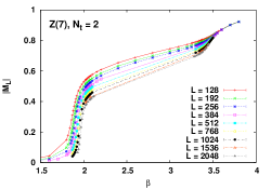
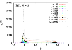
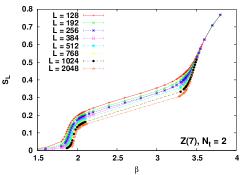
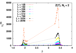
Figure 1: The two plots in the first line illustrate the method (a), while those on the second line illustrate the method (d).

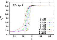
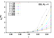
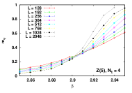
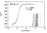
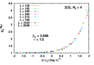
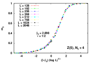
Figure 2: The two plots in the first column illustrate the method (b), while the remaining are illustrations of the method (e).

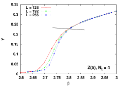
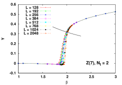
Figure 3: Behavior of the helicity modulus $\Upsilon$ for two models considered, as an illustration of the method (c); the solid line represents the curve $\Upsilon=1/(2\pi\beta\eta),\ \eta=1/4$.

2.2 Determination of the critical indices

After the determination of the $\beta_{c}$ couplings we can extract some critical indices and check the hyperscaling relation $d=2\beta/\nu+\gamma/\nu$, where $d$ is the dimension of the system. For the first transition, according to the standard FSS theory the magnetization $|M_{L}|$ at criticality should obey the relation $|M_{L}|\sim L^{-\beta/\nu}$ for $L$ large enough. Taking into account the possibility of logarithmic corrections we use

$$|M_{L}|=AL^{-\beta/\nu}\ln^{r}L\ \ \mbox{and}\ \ \chi^{(M)}_{L}=AL^{\gamma/\nu}\ln^{r}L\;,$$ (10)

where the second formula is for the susceptibility $\chi^{(M)}_{L}$, with $\gamma/\nu=2-\eta$ ($\eta$ magnetic critical index).

We apply the same procedure to the second transition with the difference that the fit with the scaling laws Eqs. (10) is to be applied to data for $M_{R}$ and $\chi_{L}^{(M_{R})}$, respectively. We found, in general, a reasonable agreement with the expectations (all the details and tables can be found in [6]).

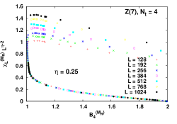
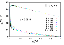
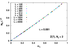
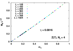
Figure 4: Correlation between $\chi_{L}^{(M_{R})}L^{\eta-2}$ and the Binder cumulant $B_{4}^{(M_{R})}$ in $Z(7)$ with $N_{t}=4$ for $\eta=0.25$ (up and left) and for $\eta=0.0816$ (up and right) for different lattice sizes. $M_{R}L^{\eta/2}$ versus $m_{\psi}$ in $Z(7)$ with $N_{t}=2$ (down and left) and in $Z(7)$ with $N_{t}=4$ (down and right) for $\eta=0.0816$ for different values of lattice size $L$.

The critical exponent $\eta$, for both transitions in these models can be calculated without knowledge of the critical temperature, building a suitable universal quantity [7]. We show in Fig. 4 some results of the behavior of these RG invariant quantities for the $Z(7)$ model with $N_{t}=2,4$. The results for the $\eta$ index is consistent with the FSS method.

3 Summary and Outlook

We have determined the two critical couplings of $Z(N=5,7,9,13)$ LGT and given estimates of the critical indices $\eta$ at both transitions. Our findings support for all $N\geqslant 5$ the scenario of three phases: a disordered phase at high temperatures, a massless or BKT one at intermediate temperatures and an ordered phase, occurring at lower and lower temperatures as $N$ increases. This matches perfectly with the $N\to\infty$ limit, i.e. the $3D$ $U(1)$ LGT (at $\beta_{s}=0$), where the ordered phase is absent. We have found that the values of the critical index $\eta$ at the two transitions are compatible with the theoretical expectations. The index $\nu$ also appears to be compatible with the value $1/2$, in agreement with RG predictions (see [6] and [8]).

Considering the determinations of the critical couplings as a function of $N$, we have also conjectured the approximate scaling for $\beta_{c}^{(1,2)}(N)$. We found that $\beta_{\rm c}^{(1)}$ converges to the $XY$ value very fast, like $\exp(-aN^{2})$ and $\beta_{\rm c}^{(2)}$ diverges like $N^{2}$ (see [6]).

On the basis of these results we are prompted to conclude that finite-temperature $3D$ $Z(N)$ LGT for $N>4$ undergoes two phase transitions of the BKT type and this model also belongs to the universality class of the $2D$ $Z(N)$ spin models, at least in the strong coupling limit $\beta_{s}=0$.

The new numerical techniques tested in these models can be useful to study other models of interest like the $3D$ $SU(N)$ LGT at finite temperature and in the strong coupling region.

- [1] V. L. Berezinsky, Sov. Phys. JETP. 32 (1971) 493.
- [2] J. M. Kosterlitz and D. J. Thouless, J. Phys. C. 6 (1973) 1181.
- [3] J. M. Kosterlitz, J. Phys. C. 7 (1974) 1046.
- [4] B. Svetitsky, L. Yaffe, Nucl. Phys. B210 (1982) 423.
- [5] R. Nelson and J.M. Kosterlitz, Phys. Rev. Lett. 39 (1977) 1201.
- [6] O. Borisenko, V. Chelnokov, G. Cortese, R. Fiore, M. Gravina, A. Papa, I. Surzhikov, Phys. Rev. E 86 (2012) 051131.
- [7] D. Loison, J. Phys.: Condens. Matter 11 (1999) L401.
- [8] O. Borisenko, V. Chelnokov, G. Cortese, R. Fiore, M. Gravina, A. Papa, Phys. Rev. E 85 (2012) 021114.