Hidden Markov Estimation of Bistatic Range From Cluttered Ultra-wideband Impulse Responses
Abstract
Ultra-wideband (UWB) multistatic radar can be used for target detection and tracking in buildings and rooms. Target detection and tracking relies on accurate knowledge of the bistatic delay. Noise, measurement error, and the problem of dense, overlapping multipath signals in the measured UWB channel impulse response (CIR) all contribute to make bistatic delay estimation challenging. It is often assumed that a calibration CIR, that is, a measurement from when no person is present, is easily subtracted from a newly captured CIR. We show this is often not the case. We propose modeling the difference between a current set of CIRs and a set of calibration CIRs as a hidden Markov model (HMM). Multiple experimental deployments are performed to collect CIR data and test the performance of this model and compare its performance to existing methods. Our experimental results show an RMSE of 2.85 ns and 2.76 ns for our HMM-based approach, compared to a thresholding method which, if the ideal threshold is known a priori, achieves 3.28 ns and 4.58 ns. By using the Baum-Welch algorithm, the HMM-based estimator is shown to be very robust to initial parameter settings. Localization performance is also improved using the HMM-based bistatic delay estimates.
Index Terms:
Ultra-wideband, hidden Markov model, localization, bistatic radar1 Introduction
A useful application of ultra-wideband (UWB) impulse radio is detection and tracking of people111In this paper, we use “people” or “person” to indicate the object being tracked. in buildings. In particular, bistatic and multistatic radar systems are used for this application [Taylor]. This is done by capturing the channel impulse response (CIR), , between transmitter/receiver pairs and detecting changes to the CIR.
This paper describes a contribution to bistatic delay (or equivalently, bistatic range) estimation. A person induces changes in the CIR starting at the bistatic delay, that is, the earliest time delay at which changes occur in the CIR due to the person being tracked. If the bistatic delay is denoted , then the bistatic range is simply the distance this multipath component has traveled, i.e., where is the speed of light. If RF energy traveled from the transmitter to the person and then to the receiver, with no additional scattering, then the bistatic range defines an ellipse on which the person is located. Thus bistatic range estimation is a key primitive of UWB tracking systems.
The primary contribution of this work is to develop a method which considers the changes which occur in a CIR at all time delays in order to estimate bistatic delay. Current published research, as described in Section 1.1, generally are first threshold-crossing methods, that is, they estimate the bistatic delay as the first delay in which a metric exceeds a threshold. As a result, they are (a) sensitive to noise in the CIR prior to the true bistatic delay, and (b) sensitive to the correct setting of the threshold parameter.
Our proposed method uses a hidden Markov model (HMM) to model the changes to the CIR as a function of time delay. The Markov chain is a progression between two states: , meaning that a person in the environment is not causing changes at the current time delay, or , meaning that a person is causing changes at the current time delay. The state of the system is observable only indirectly via the CIR, because of noise and the variability in the multipath channel. The distribution of the observations is dependent on the current state of the system, thus the system is a HMM. Using the observations and the system model, the forward-backward algorithm solves for the most likely state at any given time. The bistatic delay estimate is the time delay at which the system transitions from state 0 to state 1.
When solving for the bistatic delay, our proposed method considers all of the available data and, as we show, the error in bistatic delay estimation is reduced compared to the best thresholding scheme. Further, using a Baum-Welch algorithm, we avoid the requirement of knowing a priori the correct parameters.
1.1 Related Work
Generally, methods to estimate the bistatic delay or range first perform “background subtraction”. This means that a prior measurement, or an average of many prior measurements, of the CIR is subtracted from any current CIR measurement. These prior measurements are presumed to be made when the area is empty, i.e., with a static background.
Some work in UWB-based impulse response radar assumes that background subtraction is completely effective in removing the response due to the static environment [Thoma, Chang, Guohua, Zetik]. Some work additionally assumes that, after background subtraction, that each single multipath component caused by a person’s presence can be distinguished perfectly from the impulses caused by other people and the environment [Chang, Guohua]. In this paper, we show that ranging can still be performed when these assumptions are not true, as is often the case in a cluttered multipath environment.
One way to estimate the bistatic delay is first to perform “background subtraction”, and then to threshold on the amplitude of the difference. Zetik et al. [Zetik] describe a thresholding method which uses a simple formula for choosing an appropriate threshold value for accurate range estimation after background subtraction has been performed. Each UWB module has one transmitting and two receiving directional antennas, all relatively close to one another. This makes each UWB module approach a monostatic radar configuration. All of the sensor nodes were pointed inward toward an empty room using directional horn antennas for their experiments. In contrast, our measurements are performed in furnished office environments, and the additional clutter can make background subtraction less effective. The estimation methods described in [Zetik] will be used in this work for comparison.
Another way to estimate the delay is to perform a cross correlation of the received signal with a known target scattering profile and then to threshold the correlation values. SangHyun Chang et al. approach detection by modeling a human body’s scattering as a spectral multipath model and cross correlating this model with the received CIRs [SangHyun1, SangHyun2]. Detection is then performed using an adaptive threshold on the cross correlation. In their work they used a UWB radio similar to those used in this work but in a monostatic radar configuration. The human body spectral multipath model was obtained using empirically collected data from their UWB radio. They collected data of a moving human subject in an open field where there was little or no multipath propagation to validate their detection method [SangHyun1]. They expanded the method to tracking a human target and tested it using additional data collected from the UWB radio [SangHyun2]. The experimental data for tracking was also collected in an open field. In contrast, we use measured data from cluttered environments to show that our method is robust to the indoor multipath channel.
Our work is not the first to propose using HMMs for tracking, however, it is the first, to our knowledge, to propose using a HMM for UWB impulse radar bistatic delay estimation. Nijsure et al. used a HMM to model movement in a UWB radar-based tracking system and simulated its performance [Nijsure]. In their work, the states of the model are non-overlapping geographic regions near the radios rather than changes to the received signal. The measurements in [Nijsure] are unambiguous power delay profiles. In contrast, our HMM is used to estimate the bistatic range, with only two states, whether or not the CIR is impacted by a person at a given time delay or not. Two-state HMMs have been used in other applications, for example in detecting channel use in dynamic spectrum access [Sun]. The work in [Sun] simulated channel access by primary users and the performance of detection by secondary users, who would use the channel opportunistically, using a HMM-based estimator to detect whether a primary user is currently transmitting. Simulations showed improved detection performance for the HMM-based method compared to a threshold-based method.
1.2 Organization
This paper is organized as follows. Section 2 describes the methods proposed in this work to estimate using hidden Markov models. Section 3 describes the data collection campaigns carried out to test the proposed methods empirically. Results for our proposed methods as well as those from performing simple thresholding and the thresholding method described in [Zetik] are reported in Section 4. Finally, conclusions are discussed in Section 5.
2 Methods
2.1 Measurements
Assume that an UWB transmitter sends pulse . Due to multipath propagation, the received signal is described by
| (1) |
where and are the complex amplitude and time delay of the th path, respectively. The line of sight path delay is . The receiver radio approximately measures the channel impulse response convolved with the pulse shape. Fig. 1(a) is an example of how the transmitted pulse may follow many different paths to arrive at the receiver.
The number of multipath components seen by the receiver depends on the environment around the radios. When a person enters the environment, the person’s body will cause a new multipath component at the receiver as well as affect existing multipath components. This is illustrated in Fig. 1(b). The delay associated with this new multipath component is , which we refer to as the bistatic delay. The person also affects many for .

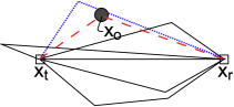
In bistatic or multistatic radar systems, the bistatic delay, described by , is used to locate and track objects near the radio transmitters and receivers. Assuming component is a single-bounce path (i.e., the path is affected by only one scatter as it travels from transmitter, to the target, and then to the receiver), the scatter is located on an ellipse with foci at the transmitter and receiver locations. That is, the locations where the scatter may be located are points where the distances from to the transmitter and receiver, and , sum to:
| (2) |
where is the speed of light.
This work seeks to accurately estimate the bistatic delay , that of the path created by the person, particularly in environments with “cluttered” impulse responses, i.e., those where individual multipath components arrive closely in time and become difficult to separate from the CIR. Estimation of is a key primitive operation for UWB impulse radar systems – estimates from multiple transmitter and receiver pairs can be used to determine possible scatter locations under a single-bounce assumption, as we explore in Section 2.7.
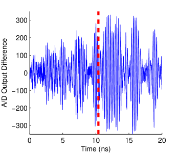
As described in Section 1.1, background subtraction is a standard method for removing the static background CIR from a current CIR measurement. However, we have found that background subtraction is not effective in cluttered environments. An example is shown in Figure 2, which shows a captured CIR subtracted from a calibration CIR over about 20 ns of time, and the true bistatic delay . Individual multipath components are indistinguishable and the signal is very noisy. If background subtraction were effective, the amplitudes prior to would be significantly lower than the amplitudes after , however, this is not the case. Better methods than simple subtraction to quantify the changes in the CIR are needed.
2.2 Quantification of Change
We describe in this section an alternative to background subtraction. We introduce a divergence measure which quantifies the change between the signal energy measured during the period when the environment is static and the current period.
We consider a discrete-sampled version of the signal energy, , given by
| (3) |
where is the sampling period. For example, in our experimental work, we use ns. Essentially, is the energy in multipath components contained within a -duration window near time delay . We call this duration window “range-bin ”. The vector is the sequence of samples. We choose to estimate the energy in each range-bin rather than using deconvolution to find the CIR. This is done to avoid the problem of deconvolution generating multiple paths when multipath experience frequency distortion [Donlan].
In this work we use the Kullback-Leibler divergence to quantify the change in the signal energy at each time . The Kullback-Leibler divergence is a measure of how many additional bits would be required to encode the samples of one distribution relative to another distribution. This is also known as relative entropy [Cover].
For continuous distributions the asymmetric KL divergence is defined as
| (4) |
where and are the probability densities of for the calibration measurements and for those under test, respectively. The symmetric KL divergence is defined as .
The observation signal, , in this model represents the difference between and of the empty room, that is, the calibration samples. In this work, this difference was calculated as the symmetric Kullback-Leibler (KL) divergence.
For the observed signal, , we use the symmetric KL divergence assuming Gaussian distributions for . This measure is given in closed form by,
| (5) |
where and are the mean and variance of during calibration, and and are the mean and variance of from the CIR measurements collected for testing. This closed form solution for is non-negative and the pdf will allow us to estimate by applying our hidden Markov model.
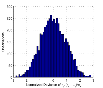
The assumption that is Gaussian is important to the closed form solution of given in equation 5. To show that follows a Gaussian distribution, each set of 10 samples of for the empty room was normalized to have a mean of 0 and a variance of 1. These samples were then aggregated for testing. With 10 sets of 90 samples of for the six radio pairs gives 5400 samples. A histogram of the normalized samples is given in Figure 3. Submitting these samples to a Kolmogorov-Smirnov test fails to reject the null hypothesis that they come from a standard normal distribution with .
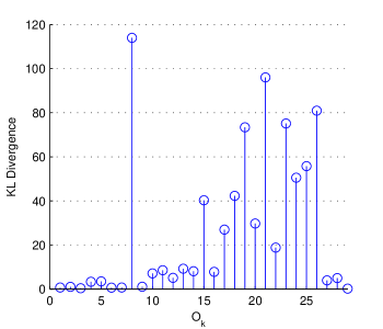
An example of an observation vector of KL divergences is given in Figure 4. This particular example is one where a first threshold-crossing method would be unable to correctly estimate the true bistatic delay, , of 15. This example shows how the assumption of easily being able to discern the background signal from the changes to the CIR can sometimes be wrong. In this case, there is a very large divergence at a time when the signals should have shown little or no difference.
Other distance measures or distributions could be applied. However, the KL-divergence and Gaussian assumption provide a standard approach for this proof-of-concept study.
2.3 CIR Changes as a Hidden Markov Model
A hidden Markov model is a special case of a Markov chain. The states of a HMM are not directly observable but may be inferred. Other signals available for observation help determine the past and current states of the system. Let be the probability of initially starting the HMM in state , is the probability of transitioning from state to state , and is the probability of observing signal given the HMM is in state , that is, . A simple illustration of a hidden Markov model is shown in Figure 5.
In the case when the observations are continuous, we use the probability density function (pdf) conditioned on the state, , for a continuous valued random variable. This is the typical way to describe a HMM for continuous-valued observations [Rabiner].

By knowing , , and , a best estimate of the current state at each time, , can be calculated. This is found by applying the forward-backward algorithm to the sequence of observation signals. When the estimated states transition from to , this gives an estimate for and indicates the presence of a person due to the changes to the observation vector.
Estimation of , where , is equivalent to estimating . Due to multipath scattering and the person’s impact on those later-arriving signals, will experience changes, or , for many . The advantage of applying a HMM is that information over all is considered when solving for rather than considering values at each independently of changes at all other .
A more thorough introduction to hidden Markov models and the algorithms used to infer information about them can be found in [Rabiner].
2.4 Continuous Observation Densities
The observations are continuous valued and their probability distribution is described by , the probability density function of given , . The HMM parameters , , and are estimated using the data collected in one room and are used as initial estimates of the HMM parameters when estimating for the other room.
The data sets , for each state , are made using the knowledge of by
| (6) |
| (7) |
Dividing the observation signals in this way assumes that there will only be one transition from state 0 to state 1 and no transitions back to state 0, that is and .
Under the assumption that given , one may also assume that and , that is, remains constant as increases. This assumption may not be true – a person’s effect will eventually diminish for large . Also, a probability of leaves little opportunity for change during optimization. To improve the model, we allow a small probability of returning from state 1 to state 0, i.e., set where is a small value greater than 0.
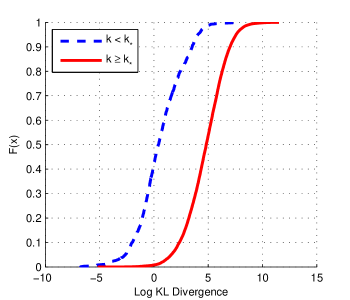
In [McCracken], no assumptions were made regarding the distribution the observations took on. The distribution was estimated by performing an Expectation Maximization algorithm to fit the data to a Gaussian mixture model. This operation was computationally expensive but effective. In this work we utilize our observation that the densities are similar to a log-normal distribution. Under this assumption, well known maximum-likelihood estimates are used for the distribution parameters. Figure 6 shows the empirical CDFs of the aggregate samples before and after for one room. The natural log is applied to in these distributions. This log-normal approximation reduces the computational load without sacrificing solving accuracy.
Initial estimates for and are given by [Rabiner, eq. (40a-b)] using the training data.
2.5 HMM Solving
The HMM parameters are described by as
| (8) |
The data from one room is used as training data to obtain an initial estimate of to begin solving for with the other room’s data, or that of the measurement room. The following describes how is estimated for the measurement room once is estimated from the training data, as described previously.
Finding , the estimate of , for the measurement room is done by solving the forward-backward algorithm. This algorithm finds the most likely state at each range-bin [Rabiner].
| (9) |
The forward-backward algorithm is different than the Viterbi algorithm, which finds the most likely state sequence over all . It may seem more appropriate to use the Viterbi algorithm to estimate when the state change occurs. The Viterbi algorithm, however, only returns a state sequence. By using the forward-backward algorithm, the additional uncertainty information of is available for each when performing localization. It should be noted that estimates for are not constrained by the room boundaries or any prior information about where the person might be located.
After estimates for are obtained, the Baum-Welch algorithm uses these estimates to update the set of HMM parameters such that
| (10) |
This is algorithm an iterative optimization on the space of to maximize .
The HMM parameters are updated over all sets of as described by Rabiner [Rabiner]. Also, is again found by estimating the distribution as log-normal using . However, is now found as
| (11) |
The algorithm continues for a predetermined number of iterations or until no longer increases more than a given tolerance with each iteration, that is, . The final estimate for is
| (12) |
This finds a local maximum in the space of possible but may not find the global maximum. The effectiveness of this algorithm is dependent on the initial values of the HMM parameters and the data itself. Other optimization algorithms exist but were not explored in this research.
2.6 First Threshold Crossing
A standard method to determine the bistatic delay, , is simply to find the first time at which is greater than a threshold. We refer to this method as first threshold crossing (FTC). Specifically the estimate of in first threshold crossing is given by
| (13) |
where is a threshold. We show the performance of this method in Figure 9 as a function of . To show how the method would perform with training, we assume that is set by using the that achieves the lowest room mean squared error (RMSE) in one room, and test performance with that in the other room.
The work presented by Zetik et al. in [Zetik] gives another method for thresholding the received CIR to estimate . This method is also used for comparison in Section 4.1.
2.7 Localization
Multiple range estimates allow localization to be performed. In this section, we describe methods for merging bistatic range estimates to obtain a position estimate. Clearly, range estimates contain errors, and any location estimator must deal with these noisy inputs.
One advantage of the HMM-based approach we propose in this paper is that it provides a ”soft” decision on the bistatic range estimate. The forward-backward algorithm quantifies the probability of each state at each time index , . If the conditional probability of state 1 increases from zero to one very quickly at time , the data is very clear that the delay bin is very likely to have been the bistatic delay. If the conditional probability increases slowly from zero to one over several delay bins, then the data is less clear. Essentially, a quantification of the probability of each delay bin being the bistatic delay is given by the rate at which the conditional probability changes.
The forward-backward algorithm finds the conditional probability of being in a given state at time . To simplify notation going forward, we will let . Since there are only two states, fully describes the probability of being in a given state at time . Also, let be defined by
| (14) |
Assuming a single-bounce model, each time delay measurement corresponds to a region on the plane given an ellipsoid with the transmitting and receiving radios at the foci. For a location estimate on a 2D plane, at least three radio pairs must give range estimates for the overlapping elliptical regions to produce a unique solution, assuming noise-free range estimates. Due to the cluttered environment, whose background UWB reflections are often much stronger than the ones caused by a person, the range estimates cannot be assumed to be noise-free. For this work, to mitigate the effect of having range estimate inaccuracy, we obtained data from six radio pairs.
Localization can be solved as an inverse problem, described by Cheng Chang et al. as a semi-linear algorithm (SLA) [Chang] which models the radio locations and range estimates as a linear function [Chang, eq. (4)]. SLA is solved using a linear least squares method. Where range estimates alone are available, solving the problem as an inverse problem makes the most sense since these estimates will often not converge perfectly due to errors and noise.
The output of the HMM, however, is more than a simple range estimate. Additional information about the probability of being in one of the two HMM states is available. This additional uncertainty at each time can be used to improve localization accuracy.
In this work, localization is solved as a forward problem as follows. We discretize space into pixels containing the area being monitored. We denote to be a quantification of the “presence” of a person in pixel . The image vector is then
| (15) |
where pixel is centered at coordinate . A person in pixel would, assuming the single-bounce model, be measured to be in range-bin for transmitter/receiver pair , where ,
| (16) |
where and are the transmitter and receiver coordinates for link and is the distance light travels during one time bin. The value is given by
| (17) |
where is the non-negative difference function of at ,
| (18) |
with . Equation (17) is the -norm of for all radio pairs at pixel . A -norm of 0, i.e. , gives a count of non-zero values and a -norm of 1 is a sum of the elements. In this work, was found to give the best performance and was the value used for the results given in Section 4.2. This -value weights the elements of such that, qualitatively, lower values are weighted more and higher values are weighted less.
Rather than using , localization can also be done using estimates . This would change the way is calculated from what is given in Equation (18) to:
| (19) |
Results for both of these methods for solving localization as a forward problem as well as solving using SLA are given in Section 4.5.
To understand pixel value more intuitively, we recall that is a soft metric for the probability that pixel is at the same bistatic range as the person, as indicated by the measurement on link . Due to the -norm in (17), is a type of average of these probabilities over all links. This method is especially useful when the measurements from a link are ambiguous, and thus for that link doesn’t change from zero to one suddenly. The uncertainty in is reflected in the presence image .
For purposes of noise reduction, we apply a 2-D Gaussian filter to image . For experiments with one person in the area, we take the coordinate of the pixel with highest (after the filtering) as the location of the person.
3 Experiment
We conduct two types of experiments for evaluation of our proposed algorithms. First, we conduct in-room experiments where transmitters and receivers are in the same room as the person being located. Second, we conduct an experiment in which the transmitter and receiver are on the other side of an interior wall of the room in which the person is located. In all experiments, we use two P220 UWB impulse radios from Time Domain, Inc., to capture CIR measurements.
3.1 In-Room Experiments
We first conduct measurements in rooms 3325 and 1280 in the Merrill Engineering Building. Two rooms are measured so that one room can be used as a training room while the other is used as an experiment room. Figures 7(a) and 7(b) describe the positions of the radios and where the person stands in each room. Room 3325 contains typical office furniture; desks, chairs, bookshelves, and computers. Room 1280 is a classroom and all of the desks and furnishings were removed from the room for the experiment. Room 1280 is also larger than room 3325, as shown in Figure 7.
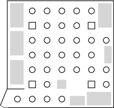
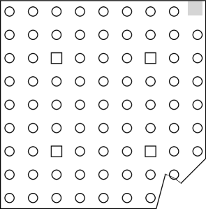
We collect both empty-room (i.e., no person in the room) calibration measurements and measurements which represent all measurements possible in a four UWB transceiver multistatic network when a person is standing at any of the possible grid points in the two rooms. Since we have only two UWB transceivers, we conduct these measurements as follows.
The two radios are placed in any of the four locations designated for the radios in the room. Ten calibration measurements of are taken when the room is empty. Then, at each of the designated points, a person stands and remains as motionless as possible while ten more measurements of are taken. After collecting measurements at all points, the two radios are moved. This process is repeated for the pair-wise radio locations. Then, the full process is repeated in the second room.
Experiment A uses the data collected in room 1208 as the training room data and the data collected in room 3325 as the data for the experiment room. Experiment B swaps the data used for the training and experiment rooms and performs the estimation again.
3.2 Through Wall Experiment
In addition to ranging and localizing a person that is in the same room as the radios, one data set is also collected to test ranging through an interior wall. Two radios are placed 1 m apart from one another and 18 cm from the wall in room 3220 in the Merrill Engineering Building at the University of Utah.
We also report the power loss due to wall penetration, in order to characterize the experiment condition. To estimate the penetration loss of the wall, the CIR is measured with the radios 4.5 m apart with both radios in room 3220. The transmitting radio is then placed on the other side of the wall in room 3230 and the receiving radio is also moved to maintain a 4.5 m separation. The CIR is measured again and the line-of-sight component of two measured CIRs are compared. The measured power loss of the wall is approximately 5 dB over the 3-5 GHz band.
The measurements are made as follows. A person stands at 30 different locations in the adjacent room 3230 while the CIR was captured 20 times per location. Figure 8 shows these two rooms with their corresponding person and radio locations. Both before and after all of these CIRs are sampled with a person present, the CIR for the empty room is captured 100 times. UWB pulse integration is also increased by a factor of 8 from what was used in the other experiments. This increases the SNR of each CIR at the cost of lowering the maximum possible sampling rate.

This through wall experiment is performed for just one radio pair, which is insufficient for localization. Instead, the purpose of this through-wall experiment is to allow us to quantify the performance of UWB impulse radio bistatic delay estimation.
4 Results
In this section, we apply the methods proposed in Section 2 to the data collected as described in Section 3. We measure the performance of our proposed HMM-based bistatic delay estimator in three ways: (1) the RMSE of the bistatic delay estimator, (2) the false negative and false positive rates, and (3) the performance of localization using our bistatic delay estimates. We compare the results of our method of estimating bistatic delay to simple thresholding as well as the thresholding method given in [Zetik].
The bistatic delay error is the difference between the person’s actual bistatic delay and the estimated bistatic delay,
We use root mean-squared error (RMSE) across all experiments to quantify average performance.
We report false negative and false positive rates for the methods studied. For bistatic delay estimation, a false negative is when there was no person’s bistatic delay detected when a person is actually present. For our HMM-based method, this corresponds to the forward-backward algorithm detecting no transition from state 0 to state 1 for the measured CIR. A false positive is when there was a bistatic delay is estimated when no person was present.
In all results, we chose a delay-bin duration of 1 ns. The choice of is a trade-off between computational requirements and quantization noise. We note that 1 ns of time corresponds to about 30 cm of distance traveled at the speed of light, approximately the width of an adult human body. Further, our results show errors significantly higher than 1 ns, and thus it has not been necessary for us to reduce further.
4.1 First Threshold Crossing
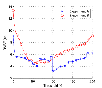
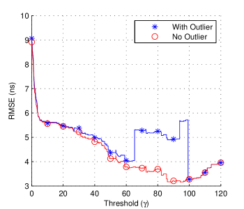
First, we test the performance of the FTC estimator as described in Section 2.6. We find the threshold that is optimal (for minimum RMSE) for the training room and then use that threshold in the testing room. From this method, a minimum RMSE of ns is achieved for Experiment A and ns for Experiment B. Next, we see what minimum could have been obtained for the testing room even if the optimal threshold for that room had been known. These absolute minimums achieved are ns and ns, respectively. Figure 9 shows how the RMSE varies as a function of the threshold. Clearly, the optimal threshold would not be known a priori for each room. Figure 9 shows the sensitivity of the RMSE to chosen threshold. For Experiment A there is a large change in the estimates with a small change to . This large change to the RMSE, occurring near values of 65 and 99, are due primarily to one set of CIRs for one point and radio pair. Without knowledge of the true values for , one would still notice the large change to with small changes to . The effect on RMSE due to this one outlier is shown in Figure 10.
There were no false negatives for the range of tested in Figure 9 for either experiment using the first threshold crossing method.
The work done by Zetik et al. [Zetik] gives a somewhat different method for thresholding the signals. The background is continually updated for each UWB node, which would correspond to a radio pair in our work, as:
| (20) |
where is the background estimate and is the newly measured CIR. The signal then used for thresholding is:
| (21) |
This removes the static background signal from the time-varying signal, which is what we wish to detect and range.
The threshold is calculated as:
| (22) |
where is the peak noise level of .
Using the method of [Zetik], described in Equations (21), (20), and (22), and the data collected, we obtain an RMSE of ns and ns for experiments A and B, respectively.
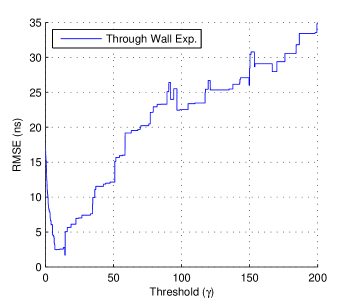
When first threshold crossing is performed on the through-wall experiment data, a plot of RMSE versus threshold is obtained and shown in Figure 11. This is comparable to those shown in Figure 9. Notice that the that achieves the optimal estimation of is different for each experiment and varies significantly. In other words, the optimal cannot be determined from data measured in a different location.
4.2 HMM-based Method
The HMM and process described in Section 2.5 are applied to the two in-room experimental data sets. The changes to RMSE for each iteration of the Baum-Welch algorithm is shown in Figure 12. The RMSE achieved after 15 iterations is ns and ns for Experiments A and B, respectively. There were no false negatives. The bias, , was ns for Experiment A and ns for Experiment B.
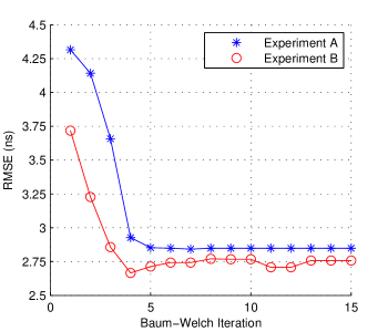
The marked improvement in RMSE from using a HMM over energy detection also comes without foreknowledge of an ideal threshold value. Although an initial estimate for is required, the Baum-Welch algorithm eliminates much of the error due to a poor estimate, as will be shown with the through-wall results 4.3. The HMM, unlike a simple threshold, takes into account the data across all time values to estimate .
The stopping condition used for the given results is to continue the Baum-Welch algorithm until there is little change to from one iteration to the next. That is . Experiment A converges, using this metric, after 9 iterations and Experiment B after 14 iterations.
4.3 Through-wall experiment
Our proposed HMM method is also applied to data captured through a wall dividing two rooms as described in Section 3.2. Observation vectors are calculated using all of the available empty room CIRs and CIRs with a person present. With the observation vectors and an initial estimate for the HMM parameters , estimates for can be found.
Using the that is found to be optimum for any one of the three environments as the initial for any of the other environments results in the same solution for from the Baum-Welch algorithm. This is illustrated using the through wall data. For the through wall data, there are three choices of , two obtained from the data collected from the two in-room experiments described in Section 3.1 and one from the data and known locations of this through wall data. The obtained from the through wall data could not be used in a production system because it is derived using a knowledge of . If is known, there is no reason to use it to find to then estimate . It is used here solely for illustrative purposes.
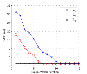
Figure 13 shows the bistatic delay RMSE at each iteration of the Baum-Welch algorithm for the three different choices for at the first iteration. The choice of greatly influences the RMSE at first, but the effect of the choice is ultimately negated by the Baum-Welch algorithm. The final RMSE in all three cases is 1.33 ns.
This final error is better than the results obtained with the subject in the same room as the radios. There are several reasons for this.
-
1.
Number of samples: Many more samples of the empty room were collected and used in determining the KL-divergences in the through-wall experiment (200) compared to the in-room experiments (10). These additional samples help to reduce the noise in the observation vectors. The effect of choosing different empty room samples is explored further below.
-
2.
Additional integration: Additional signal integration was done in sampling to reduce noise in the CIRs because of the additional path loss in the through-wall experiment.
To show the effect of the number of empty room samples on the performance of the ranging estimation (item 1 above), we run an experiment in which we reduce the number of empty-room samples used in the through-wall experiment. Here, we calculate observation vectors of KL-divergences using sets of 20 sequential empty room samples. From the two sets of 100 empty room samples, this leads to 162 sets of sequential samples. The initial choice of was the same used in Experiment A. The overall RMSE was calculated for each of these sets of empty room samples. Two of the 30 person locations had a wide variation in their range estimate depending on which set of empty room samples was chosen. Figure 14 shows the empirical CDF of the final RMSE obtained using each of these sets of empty room samples both with and without these two person locations.
For the trials using all person locations, 12.3% of the trials resulted in an RMSE better than the 1.33 ns achieved using all of the empty room samples together. The overall RMSE for all of the trials using 20 empty room samples is 4.19 ns. This illustrates that, on average, using a fewer number of empty room samples degrades performance.
4.4 False Positives
Testing for false positives, or non-zero estimates of in empty room samples, was also performed. The Baum-Welch algorithm was not performed on these samples, that is, no updating of the HMM parameters was done for re-estimation of .
False positives were tested by randomly dividing the set of empty-room samples into the known empty-room and possible point sample sets. Due to the limited sample sizes for empty-room samples, this random set division allows us to simulate how false positive tests might perform using different sample sets that aren’t available. For each radio pair, the available samples were divided evenly between the known empty-room sample set and the possible point sample set. These two sets were used to find the observation vector of KL divergences, which the HMM uses to estimate .
For each of the six transmitter/receiver pairs for each of the two rooms, 1000 trials were performed using the random subset division described for a total of 12,000 trials. Of these a total of 50 trials resulted in false positives, that is, a false positive rate. We note that over half of the false positives come from a single transmitter/receiver pair in one of the rooms. Notably, this pair had just 10 empty-room samples available for testing. This is the fewest number of empty-room samples for any transmitter receiver pair.
4.5 Localization
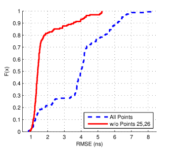
Results for localization are given for both the forward method described in Section 2.7 and the SLA described described by Cheng Chang et al. [Chang]. The forward solving method is done in two ways, first using where and second using only the range estimates, , without the additional information of the probability of being in a given state.
The SLA described by Cheng Chang et al. only uses range estimates for localization. A summary of the results of each localization method with its available information is given in Tables I and II. All values are given in cm.
| Forward | SLA | ||
|---|---|---|---|
| All Info | Range Only | Range Only | |
| Rm 3325 | 36 | 155 | 165 |
| Rm 1208 | 24 | 75 | 194 |
| Forward | SLA | ||
|---|---|---|---|
| All Info | Range Only | Range Only | |
| Rm 3325 | 16 | 67 | 159 |
| Rm 1208 | 16 | 29 | 172 |
The forward solving method described here gives location estimates that are significantly better than those from the SLA described by Cheng Chang et al. Taking into account rather than using alone also improves the location estimates for the forward solving method.
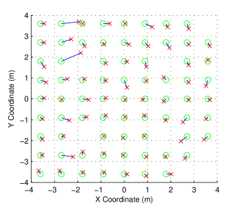
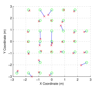
Figures 15 and 16 describe the true person locations, as shown previously in Figure 7, and the estimates for those locations using the forward solving method with all available information.
5 Conclusions
In this paper, we introduce and experimentally-verify a hidden Markov model-based algorithm for estimating the bistatic delay in an UWB impulse radar system. We show the proposed algorithm achieves a lower RMSE than first threshold crossing methods for highly cluttered multipath environments. Applying the Baum-Welch algorithm allows the proposed estimator to adapt its parameters to be best for the particular environment. We show the algorithm is robust to initialization parameters derived from a different environment.
Compared to using the first threshold crossing estimate of , our method reduces error by almost half. Since these estimates of the person’s bistatic delay are used directly in tracking algorithms, we expect to similarly improve UWB-based localization performance.
The forward solving method described here for localization using the probabilities was very effective, achieving a median error of 18 cm.
One primary limitation of the algorithm as proposed is that it assumes only one person is causing changes to the CIR. To account for more people, future work must expand the HMM-based estimator to estimate a bistatic delay for each person in the environment. Research must determine what methods to use in the multiple person case, for example, if more states are needed in the Markov model, or if joint estimation the number of people and their bistatic delays improves performance.
![[Uncaptioned image]](/html/1212.1080/assets/x19.png) |
Merrick McCracken received the B.S. in Computer Engineering (2009) from Brigham Young University - Idaho and the M.S. in Electrical and Computer Engineering (2011) from the University of Utah. He is a recipient of of the Science, Mathematics & Research for Transformation Scholarship (2010) through the US Department of Defense. He is currently working as a Ph.D. student in the Sensing and Processing Across Networks (SPAN) Lab at the University of Utah. |
![[Uncaptioned image]](/html/1212.1080/assets/x20.png) |
Neal Patwari received the B.S. (1997) and M.S. (1999) degrees from Virginia Tech, and the Ph.D. from the University of Michigan, Ann Arbor (2005), all in Electrical Engineering. He was a research engineer in Motorola Labs, Florida, between 1999 and 2001. Since 2006, he has been at the University of Utah, where he is an Associate Professor in the Department of Electrical and Computer Engineering, with an adjunct appointment in the School of Computing. He directs the Sensing and Processing Across Networks (SPAN) Lab, which performs research at the intersection of statistical signal processing and wireless networking. Neal is the Director of Research at Xandem, a Salt Lake City-based technology company. His research interests are in radio channel signal processing, in which radio channel measurements are used to benefit security, networking, and localization applications. He received the NSF CAREER Award in 2008, the 2009 IEEE Signal Processing Society Best Magazine Paper Award, and the 2011 University of Utah Early Career Teaching Award. He is an associate editor of the IEEE Transactions on Mobile Computing. |