Anomalous currents in driven XXZ chain with boundary twisting at weak coupling or weak driving

Abstract

The spin $1/2$ $XXZ$ chain driven out of equilibrium by coupling with boundary reservoirs targeting perpendicular spin orientations in $XY$ plane, is investigated. The existence of an anomaly in the nonequilibrium steady state (NESS) at the isotropic point $\Delta=1$ is demonstrated both in the weak coupling and weak driving limits. The nature of the anomaly is studied analytically by calculating exact NESS for small system sizes, and investigating steady currents. The spin current at the points $\Delta=\pm 1$ has a singularity which leads to a current discontinuity when either driving or coupling vanish, and the current of energy develops a twin peak anomaly. The character of singularity is shown to depend qualitatively on whether the system size is even or odd.

I Introduction

The coupling of a quantum system with an environment or under a continuous measurement is often modelled via a quantum Master equation in the Lindblad form Petruccione ; PlenioJumps . Unlike a quantum system evolving coherently, the time evolution of which depends on the initial state, a quantum system with pumping tends to a nonequilibrium steady state, independent of the initial conditions. Recently there has been a large interest in investigating chains of quantum spins driven towards nonequilibrium steady states by applying gradients (pumping) at the edges. An important role in these studies is played by the one dimensional driven XXZ chain. The equilibrium XXZ model remains a subject of intensive investigations via various methods reviewBrenig07 ; zotos ; KlumperLectNotes2004 ; Bosonisation ; SchollwoeckRev05 . In experiments, many transport characteristics in quasi one-dimensional spin chain materials can be measured HessBallistic2010 . In the context of dissipative dynamics, recent numerical and analytic studies of a driven XXZ chain show a number of remarkable features like long range order and quantum phase transitions far from equilibrium TP_Pizorn08 , negative differential conductivity of spin and energy BenentiPRB2009 ; ZunkovichJStat2010ExactXY , solvability Pros08 ; ProsenExact2011 ; MPA etc..

Recently it was shown that an isotropic point $\Delta=1$, a weakly driven $XXZ$ spin chain has an anomalous spin transport znidaricprl2011 . The current-carrying nonequilibrium steady state was obtained by bringing an $XXZ$ spin chain in contact with reservoirs aligning the boundary spins along the $Z$-axis. The boundary gradient was small, which allows to think in terms of linear response of a system to the weak perturbation along the anisotropy axis.

From a standard theory of linear response KuboBook one expects that the result of linear response will not depend on a form of boundary perturbation as long as it remains sufficiently weak. Respectively, an anomaly seen with one type of perturbation, should be visible with another type of perturbation as well. On the other hand, the linear response theory is valid for system in thermodynamic equilibrium at a certain temperature, while the driven chains with dissipative boundary driving are intrinsically nonequilibrium systems. At ”zero gradient” the NESS describes a system without currents, in a maximally mixed quantum state, which corresponds to a Gibbs ensemble with an infinite temperature. To test further the linear response regime in a situation of a nonequilibrium, we investigate a weakly driven $XXZ$ chain, where the weak boundary gradient at the boundaries is applied in the $XY$ direction, transverse to the anisotropy axis Lindblad2011 ; PopkovXYtwist . Note that there are two complementary ways of realizing a weak drive in a Master equation formalism: (i) to set a weak boundary gradient, but finite or strong coupling to boundary reservoirs (ii) to set a weak coupling to reservoir, but finite or strong boundary gradient.

Interestingly, in both contexts (either weak gradient $\kappa\ll 1$ or weak coupling $\Gamma\ll 1$) we see a distinct anomaly in the NESS. The anomaly becomes a singularity as $\Gamma\rightarrow 0$ or $\kappa\rightarrow 0$. of the magnetization current in the isotropic point $\Delta=1$. For weak coupling the anomaly sets in for $N\geq 2$ and for weak driving for $N\geq 4$. The presence of an anomaly is seen in practically all observables. In present communication we focus on singular behaviour of the steady currents of spin $j$ and energy $J^{E}$, and one-point correlations at the boundaries. The full analytic treatment is reported for spin current. In the limit $\kappa\rightarrow 0$ or $\Gamma\rightarrow 0$ we observe a non-analyticity in the dependence $j(\Delta)$: the spin current is an analytic smooth function of $\Delta$ everywhere except at isotropic point $\Delta=1$ where its value is different. The nature of singularity, in addition, depends on the parity of system size, namely on whether the system size is an even or an odd number.

Other observables e.g. current of energy, density profiles etc. also have a singular behaviour at $\Delta=\pm 1$. Thus, we can complement the result of Znidaric znidaricprl2011 with prediction of further anomalies at the isotropic point. In particular, we demonstrate that the energy current also develops an anomaly at the isotropic point, but with a different scaling and of a qualitatively different form.

The plan of the paper is the following. We introduce the model in the Sec.II. The cases of weak coupling and weak driving are treated separately in Sec.III and Sec.IV. In the conclusion we summarize our findings.

II The model

We study an open chain of $N$ quantum spins in contact with boundary reservoirs. The time evolution of the reduced density matrix $\rho$ is described by a quantum Master equation in the Lindblad form Petruccione , PlenioJumps (here and below we set $\hbar=1$)

$$\frac{\partial\rho}{\partial t}=-i\left[H,\rho\right]+\Gamma_{L}\mathcal{L}_{L}[\rho]+\Gamma_{R}\mathcal{L}_{R}[\rho],$$ (1)

where $H$ is the Hamiltonian of an open $XXZ$ spin chain with an anisotropy $\Delta$

$$H=\sum_{k=1}^{N-1}\left(\sigma_{k}^{x}\sigma_{k+1}^{x}+\sigma_{k}^{y}\sigma_{k+1}^{y}+\Delta\sigma_{k}^{z}\sigma_{k+1}^{z}\right),$$ (2)

while $\mathcal{L}_{L}$ and $\mathcal{L}_{R}$ are Lindblad dissipators favoring a relaxation of boundary spins $k=1$ and $k=N$ towards states described by density matrices acting on a single site $\rho_{L}$ and $\rho_{R}$, i.e. $\mathcal{L}_{L}[\rho_{L}]=0$ and $\mathcal{L}_{R}[\rho_{R}]=0$. The Lindblad actions $\mathcal{L}_{L}$ and $\mathcal{L}_{R}$ are chosen in the form

$$\mathcal{L}_{L}[\rho] =-\frac{1}{2}\sum_{m=1}^{2}\left\{\rho,W_{m}^{{\dagger}}W_{m}\right\}+\sum_{m=1}^{2}W_{m}\rho W_{m}^{{\dagger}},$$

$$\mathcal{L}_{R}[\rho] =-\frac{1}{2}\sum_{m=1}^{2}\left\{\rho,V_{m}^{{\dagger}}V_{m}\right\}+\sum_{m=1}^{2}V_{m}\rho V_{m}^{{\dagger}},$$

where $W_{m}$ and $V_{m}$ are polarization targeting Lindblad operators, which act on the first and on the last spin respectively, $W_{1}=\sqrt{\frac{1-\kappa}{2}}(\sigma_{1}^{z}+i\sigma_{1}^{x})$, $W_{2}=\sqrt{\frac{1+\kappa}{2}}(\sigma_{1}^{z}-i\sigma_{1}^{x})$, $V_{1}=\sqrt{\frac{1+\kappa}{2}}(\sigma_{N}^{y}+i\sigma_{N}^{z})$, $V_{2}=\sqrt{\frac{1-\kappa}{2}}(\sigma_{N}^{y}-i\sigma_{N}^{z})$. In absence of the unitary term in (1) the boundary spins relax with a characteristic time $\Gamma_{L}^{-1},\Gamma_{R}^{-1}$ BoundaryRelaxationTimes to specific states described via the one-site density matrices $\rho_{L}$ and $\rho_{R}$, satisfying $\mathcal{L}_{L}[\rho_{L}]=0$ and $\mathcal{L}_{R}[\rho_{R}]=0$, where

$$\rho_{L} =\frac{1}{2}\left(I-\kappa\sigma_{1}^{y}\right)$$

$$\rho_{R} =\frac{1}{2}\left(I+\kappa\sigma_{N}^{x}\right).$$

From the definition of a one-site density matrix $\rho_{one-site}=\frac{1}{2}\left(I+{\textstyle\sum}\langle\sigma^{\alpha}\rangle\sigma^{\alpha}\right)$, we see that the Lindblad superoperators $\mathcal{L}_{L}$ and $\mathcal{L}_{R}$ indeed try to impose a twisting angle of $\pi/2$ in $XY$ plane between the first and the last spin TwistingRemark . The twisting gradient drives the system in a steady-state with currents. In the following we restrict to a symmetric choice

$$\Gamma_{L}=\Gamma_{R}=\Gamma$$ (3)

for spin current while $\Gamma_{L}\neq\Gamma_{R}$ is chosen for studying the energy currentenergyRemark . The parameter $\kappa$ determines the amplitude of the gradient between the left and right boundary, and therefore plays a fundamentally different role from the coupling strength $\Gamma$. The limits $\kappa=1$ and $\kappa\ll 1$ will be referred to as the strong driving and weak driving case respectively. The two limits describe different physical situations as exemplified in other NESS studies. For symmetric choice (3) the steady state has a global symmetry PopkovXYtwist ,SP2012

$$\rho(N,\Delta)=\Sigma_{x}U_{rot}R\rho(N,\Delta)RU_{rot}^{+}\Sigma_{x},$$ (4)

where $R(A\otimes B\otimes...\otimes C)=(C\otimes....\otimes B\otimes A)R$ is a left-right reflection, and the diagonal matrix $U_{rot}=diag(1,i)^{\otimes_{N}}$ is a rotation in $XY$ plane, $U_{rot}\sigma_{n}^{x}U_{rot}^{+}=\sigma_{n}^{y}$, $U_{rot}\sigma_{n}^{y}U_{rot}^{+}=-\sigma_{n}^{x}$, and $\Sigma_{x}=(\sigma^{x})^{\otimes_{N}}$. In addition, there are further transformations, see PopkovXYtwist for details, relating the NESS for positive and negative $\Delta$,

$$\rho(2N,-\Delta)=U\rho^{\ast}(2N,\Delta)U$$ (5)

$$\rho(2N+1,-\Delta)=\Sigma_{y}U\rho^{\ast}(2N+1,\Delta)U\Sigma_{y},$$ (6)

where $\Sigma_{y}=(\sigma^{y})^{\otimes_{N}},$ and $U={\textstyle\prod\limits_{n\,odd}}\otimes\sigma_{n}^{z}$, and conjugate is taken in the basis where $\sigma^{z}$ is diagonal. In view of the above symmetries, below we restrict to the case of positive $\Delta\geq 0$.

We shall consider two particular limits:

A) weak coupling, $\Gamma\ll 1$, strong driving (large gradient) $\kappa=1$).

B) weak gradient $\kappa\ll 1$, strong coupling $\Gamma^{-1}\ll 1$

Both limits show qualitatively similar singular behaviour as $\kappa\rightarrow 0$ or $\Gamma\rightarrow 0$, at the isotropic point $\Delta=1$ as demonstrated below.

III Case of strong driving $\kappa=1$ and weak coupling $\Gamma\ll 1$

To investigate the system in the case of large boundary gradients $\kappa=1$ and weak coupling $\Gamma\ll 1$, we solve the linear system of equations which determine the full steady state, analytically, making use of the global symmetry (4) SP2012 which decreases the number of unknown variables by roughly a factor of $2$. For $N=2,3,4$ we have indeed $9$, $31$ and $135$ real unknowns, respectively, instead of $2^{2N}-1$ real unknowns for the full Hilbert space. For $N=2$ the current $j(\Gamma,\Delta)$ is readily obtained as

$$j(\Gamma,\Delta)=\frac{8\Gamma^{4}(3+6\Gamma^{2}+2\Delta^{4})}{24\Gamma^{6}+3(\Delta^{2}-1)^{2}+2\Gamma^{4}(7\Delta^{4}+30)+\Gamma^{2}(2\Delta^{4}+13\Delta^{2}+30)},$$ (7)

from which we see that at the points $\Delta=\pm 1$ and in the small coupling limit, it scales quadratically with $\Gamma$,

$$\lim_{\Gamma\rightarrow 0}\lim_{\Delta\rightarrow 1}\left.\frac{j(\Gamma)}{\Gamma^{2}}\right|_{N=2}=\frac{8}{9}.$$ (8)

Note, however, that for $\Delta\neq\pm 1$ the current scales as $\Gamma^{4}$, i.e

$$\lim_{\Gamma\rightarrow 0}\left.\frac{j(\Gamma)}{\Gamma^{4}}\right|_{N=2}=\frac{8(2\Delta^{2}+3)}{3(\Delta^{2}-1)^{2}}$$ (9)

For $N=3$ the current $j(\Gamma,\Delta)$ at $\Delta=1$, still scales as $\Gamma^{2}$,

$$\lim_{\Gamma\rightarrow 0}\lim_{\Delta\rightarrow 1}\left.\frac{j(\Gamma)}{\Gamma^{2}}\right|_{N=3}=\frac{16}{9}$$ (10)

but a different scaling behavior, with respect to $N=2$ case, is obtained for other $\Delta$ points, where the $j$ is found to scale also quadratically,

$$\lim_{\Gamma\rightarrow 0}\left.\frac{j(\Gamma)}{\Gamma^{2}}\right|_{N=3}=\frac{6\Delta\left(9\Delta^{2}+59\right)}{9\Delta^{4}+155\Delta^{2}+416},$$ (11)

Taking the limit $\Delta\rightarrow 1$ in the above, we obtain

$$\lim_{\Delta\rightarrow 1}\lim_{\Gamma\rightarrow 0}\left.\frac{j(\Gamma)}{\Gamma^{2}}\right|_{N=3}=\frac{102}{145},$$ (12)

different from (10). Consequently, the limits $\Delta\rightarrow 1$ and $\Gamma\rightarrow 0$ do not commute. In more details, we have

$$\lim_{\Delta\rightarrow 1}\left.\frac{j(\Gamma)}{\Gamma^{2}}\right|_{N=3}=\frac{16(3+\Gamma^{2})}{27+52\Gamma^{2}+12\Gamma^{4}},$$ (13)

from which Eq(10) is straightforwardly obtained. Alternatively, one can see the presence of a singularity at all even orders of expansion of $j(\Gamma)$: starting from the order $4$ of the expansion, all even terms $\left.(\partial^{m}j_{0}(\Gamma,\Delta)/\partial\Gamma^{m})\right|_{\Gamma=0}$ contain poles at $\Delta=\pm 1$ of the type $1/(\Delta^{2}-1)^{m-2}$, e.g.

$$\frac{\partial^{m}j_{0}(\Gamma,\Delta)}{\partial\Gamma^{m}}|_{\Gamma=0}=\frac{(-1)^{\frac{m}{2}+1}}{(\Delta^{2}-1)^{m-2}}Q(\Delta)$$ (14)

with $Q(\Delta)$ a rational function which is regular at points $\Delta=\pm 1$.

For $N=4$ one can see that the current at $\Delta=\pm 1$ scales with $\Gamma$ as:

$$\lim_{\Delta\rightarrow\pm 1}\left.\frac{j(\Gamma)}{\Gamma^{2}}\right|_{N=4}=\frac{8(27+46\Gamma^{2}+10\Gamma^{4})}{3(27+135\Gamma^{2}+144\Gamma^{4}+28\Gamma^{6})}$$ (15)

from which it follows that in the small coupling limit the current reduces to

$$\lim_{\Gamma\rightarrow 0}\lim_{\Delta\rightarrow\pm 1}\left.\frac{j(\Gamma)}{\Gamma^{2}}\right|_{N=4}=\frac{8}{3}.$$ (16)

At all other points $\Delta\neq\pm 1$, however, the current scales as for the $N=2$ case, e.g

$$\lim_{\Gamma\rightarrow 0}\left.\frac{j(\Gamma)}{\Gamma^{4}}\right|_{N=4}=O\left(\frac{1}{(\Delta^{2}-1)^{2}}\right).$$ (17)

Although analytical expressions of the current are very difficult to obtain for larger values of $N$ (e.g. $N>4$), we can infer from numerical calculations that similar behavior exist also in these more complicated cases. Indeed, from the exact expressions reported above and from direct numerical calculations it is possible to extrapolate the values of the current for arbitrary $N$ at the points $\Delta\pm 1$ in the small coupling limit as:

$$\lim_{\Gamma\rightarrow 0}\lim_{\Delta\rightarrow\pm 1}\left.\frac{j(\Gamma)}{\Gamma^{2}}\right|_{N}=\frac{8}{9}(N-1),$$ (18)

hinting at $\Gamma=0$ becoming a singular point in the thermodynamic limit. One can readily see that our conjecture (18) coincides with the exact values reported in Eqs. (8), (10), (16) for cases $N=2,3,4$, respectively. Moreover, numerical results provides us a high confidence about the validity of Eq. (18) for arbitrary $N$. More precisely, we find from direct numerical solutions of the LME that the peaks of the current for $N=7,8,9$ at $\Gamma=10^{-5}$ are: $5.3333,6.2222,7.111$, respectively, in perfect agreement with the prediction of Eq.(18). Also note from Fig. 1 that the numerical values of the current peaks depicted in panels (c),(d) for cases $N=5,6$ ($3.5556$ and $4.4444$, respectively) are in excellent agreement with Eq. (18). Moreover, using the Matrix Product Ansatz MPA , we were able to check the conjecture (18) analytically up to sizes $N=100$ (details to be published elsewhere). From the physical point of view, Eq. (18) is quite interesting because it implies that in the weak coupling limit an addition of an extra spin to a finite chain contributes to the total current by a ”quantum” of $8\Gamma^{2}/9$. Since the spin current is bounded, the Eq.(18) hints at a singularity in $\Gamma=0$ point in the thermodynamic limit $N\rightarrow\infty$. Further details and an analytical proof of (18) will be presented elsewhere.

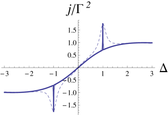
(a)

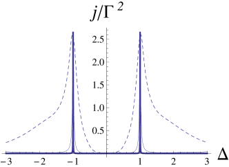
(b)

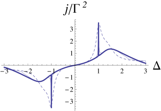
(c)

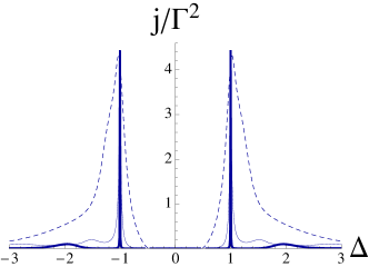
(d)

Figure 1: Typical dependence of renormalized current $j/\Gamma^{2}$ versus anisotropy for small couplings $\Gamma$ and odd system size (Panels (a),(c)) and for even system size (Panels (b),(d)). Dashed, thin, and thick lines correspond to $\Gamma=10^{-1},10^{-2},10^{-3}$ respectively. The system size is $N=3,4,5,6$ for Panels (a),(b),(c) and (d), respectively. The curves are obtained by a numerical solution of the LME.

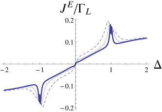
(a)

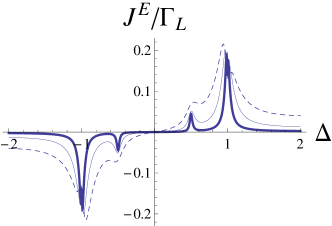
(b)

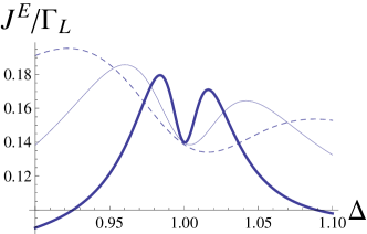
(c)

Figure 2: Dependence of renormalized energy current $j/\Gamma_{L}$ versus anisotropy for small couplings $\Gamma_{L},\Gamma_{R}$ and system size $N=3$ (Panel (a)) and for $N=4$ (Panel (b)). Dashed, thin, and thick lines correspond to $\Gamma_{L}=0.1,0.05,0.02$ respectively, while $\Gamma_{R}=\Gamma_{L}/2$. The curves are obtained by numerical solution of the LME. The peaks for $N=4$ are at the points $\Delta=\pm 0.5,\pm 1$. Panel (c). A closeup view of the Panel(a), demonstrating double peak structure close to $\Delta=1$.

One naturally expects that the noticed singular behaviour of the driven $XXZ$ model at the isotropic point is not restricted to the magnetization current but can be seen for other observables as well. Here we show that the energy current is also anomalous at the isotropic point. Our purpose here, in addition, is to demonstrate, that the global symmetry (4) is not crucial for singularity, because the energy current only flows if the symmetry (4) is broken. Indeed, the energy current operator $\hat{J}_{n}^{E}(\Delta)$, defined through the local Hamiltonian term $h_{n,n+1}$ as $dh_{n,n+1}/dt=\hat{J}_{n-1}^{E}(\Delta)-\hat{J}_{n}^{E}(\Delta),$

$$\hat{J}_{n}^{E}(\Delta)=-\sigma_{n}^{z}\hat{\jmath}_{n-1,n+1}+\Delta(\hat{\jmath}_{n-1,n}\sigma_{n+1}^{z}+\sigma_{n-1}^{z}\hat{\jmath}_{n,n+1})$$

where $\hat{\jmath}_{n,m}=2(\sigma_{n}^{x}\sigma_{m}^{y}-\sigma_{n}^{y}\sigma_{m}^{x})$, changes sign under the action of (4), $(RU_{rot}^{+}\Sigma_{x})\hat{J}_{n}^{E}(RU_{rot}^{+}\Sigma_{x})$ $=-\hat{J}_{n}^{E}$ and therefore in the stationary state it is strictly zero $\langle\hat{J}_{n}^{E}\rangle=J^{E}=0$ (as a local integral of motion, the energy current does not depend on the choice of the bond $n$). Lifting up the symmetric choice for the couplings to the left and right reservoirs in (1), i.e., considering the Lindblad equation (1) with $\Gamma_{L}\neq\Gamma_{R}$ we break the symmetry (4) and the energy current becomes permissible, see also PopkovLivi . The current of energy for small couplings $\Gamma_{L},\Gamma_{R}\ll 1,$ with a fixed ratio $\Gamma_{L}/\Gamma_{R}=const$ shows, again, an approach to a singularity in the isotropic point, but with a different scaling, $J^{E}(\Delta=1)=O(\Gamma_{L})$, and qualitatively different behaviour, see Fig.2. Indeed, the anomaly of energy current at the isotropic point has a shape of a twin peak, which, as $\Gamma_{L}$ decreases, becomes more and more narrow, see Fig.2(c), and for $\Gamma_{L}\rightarrow 0$ develops a twin peak singularity. For $N=4$ we see a twin peak singularity at $\Delta=1$ and a single peak singularity at $\Delta=0.5$, illustrated on Fig.2(b). Unlike the spin current which is the odd (even) function of $\Delta$ for odd (even) number of sites, the energy current is always an odd function of $\Delta$. These parity features are direct consequences of the mappings (5) and (6), see also PopkovXYtwist . Further details will be discussed elsewhere. Here we just mention another observable which has a singularity at the isotropic point, also in the symmetric case $\Gamma_{L}=\Gamma_{R}=\Gamma$: it is the actual value of magnetizations at the boundaries: $\langle\sigma_{1}^{x}\rangle,\langle\sigma_{N}^{x}\rangle$, $\langle\sigma_{1}^{y}\rangle$,$\langle\sigma_{N}^{y}\rangle$, which, as $\Gamma\rightarrow 0$, remain finite at $\Delta=1$, and attain different values at the point $\Delta 1\pm 0$, data not shown. Interestingly, this singularity cancels in the difference $\Delta x=\langle\sigma_{1}^{x}-\sigma_{N}^{x}\rangle$ and $\Delta y=\langle\sigma_{1}^{y}-\sigma_{N}^{y}\rangle$: the actual magnetization differences $\Delta x,\Delta y$ are regular at $\Delta=1$.

At this point one might suspect, that the singularities in the currents of spin and energy are just artefacts (or direct consequences) of the singular behaviour of the boundary gradients. To eliminate the influence of the irregular behaviour of the boundary gradients, in the next section we consider another limit, where we control not only the boundary gradients $\Delta x,\Delta y$, but also the individual magnetizations at the boundaries $\langle\sigma_{1}^{x}\rangle,\langle\sigma_{1}^{y}\rangle$, $\langle\sigma_{1}^{z}\rangle$,$\langle\sigma_{N}^{x}\rangle,\langle\sigma_{N}^{y}\rangle$, $\langle\sigma_{N}^{z}\rangle$, which become exactly equal to $0,-\kappa,0,\kappa,0,0$, respectively.

IV Case of weak boundary gradients and strong coupling

In this section we investigate the weak gradient and strong coupling case ($\kappa\ll 1$,$\Gamma^{-1}\ll 1$) by means of the perturbative approach for the LME in powers of $\Gamma^{-1}$, developed in PopkovXYtwist . Note that while in the standard derivation of the Lindblad Master equation one usually assumes the coupling to the reservoirs to be weakPetruccione ,Wichterich07 , in the ancilla Master equation construction ClarkPriorMPA2010 this restriction is lifted and the effective coupling can become arbitrarily strong. We also remark that the uniqueness of the nonequilibrium steady state for any coupling $\Gamma$ is guaranteed by the completeness of the algebra, generated by the set of operators $\{H,V_{m},W_{m},V_{m}^{+},W_{m}^{+}\}$ under multiplication and addition EvansUniqueness , and is verified straightforwardly along the lines ProsenUniqueness . We search for a stationary solution of the Lindblad equation in the form of a perturbative expansion in $\Gamma^{-1}$,

$$\rho(\Delta,\Gamma)=\sum_{k=0}^{\infty}\left(\frac{1}{2\Gamma}\right)^{k}\rho_{k}(\Delta),$$ (19)

where $\rho_{0}(\Delta)=\lim_{\Gamma\rightarrow\infty}\rho(\Delta,\Gamma)$ satisfies $\mathcal{L}_{LR}[\rho_{0}(\Delta)]=0$. Here and below we denote by $\mathcal{L}_{LR}[.]$ the sum of Lindblad boundary actions $\mathcal{L}_{LR}[.]=\mathcal{L}_{L}[.]+\mathcal{L}_{R}[.]$. This enforces a factorized form

$$\rho_{0}(\Delta,\kappa)=\rho_{L}\otimes\left(\left(\frac{I}{2}\right)^{\otimes_{N-2}}+M_{0}(\Delta,\kappa)\right)\otimes\rho_{R},$$ (20)

where $\rho_{L}$ and $\rho_{R}$ are one-site density matrices given by (II),(II) which satisfy $\mathcal{L}_{L}[\rho_{L}]=0$, $\mathcal{L}_{R}[\rho_{R}]=0$ and $M_{0}(\Delta,\kappa)$ is a matrix to be determined self-consistently later. Below we shall drop $\Delta$- and $N$-dependence in $\rho_{k}$ and $M_{k}$ for brevity of notations. Substituting (19) into (1), and comparing the orders of $\Gamma^{-k}$, we obtain recurrence relations

$$i[H,\rho_{k}]=\frac{1}{2}\mathcal{L}_{LR}\rho_{k+1}\,\,k=0,1,2...$$ (21)

A formal solution of the above is $\rho_{k+1}=-2\mathcal{L}_{LR}^{-1}(Q_{k+1})$ where $Q_{k+1}=-i[H,\rho_{k}]$. Note however that the operator $\mathcal{L}_{LR}$ has a nonempty kernel subspace, and is not invertible on the elements from it. The kernel subspace $\ker(\mathcal{L}_{LR})$ consists of all matrices of type $\rho_{L}\otimes A\otimes\rho_{R}$ where $A$ is an arbitrary $2^{N-2}\times$ $2^{N-2}$ matrix. Therefore $\rho_{k+1}$ exists only if $[H,\rho_{k}]\cap\ker(\mathcal{L}_{LR})=\varnothing$, which in our case reduces to a requirement of a null partial trace, see PopkovXYtwist .

$$Tr_{1,N}([H,\rho_{k}])=0,\,\,k=0,1,2....$$ (22)

which we call secular conditions. Finally, $\rho_{k+1}$ is defined up to an arbitrary element from $\ker(\mathcal{L}_{LR})$, so we have

$$\rho_{k+1}=2\mathcal{L}_{LR}^{-1}(i[H,\rho_{k}])+\rho_{L}\otimes M_{k+1}\otimes\rho_{R},\;\;k=0,1,2...$$ (23)

Eqs. (20), (22) and (23) define a perturbation theory for the Lindblad equation (1) for strong couplings. At each order of the perturbation theory the secular conditions (22) must be satisfied, which impose constraints on $M_{k}$. Our aim here is to determine the exact NESS in the limit $\Gamma\rightarrow\infty$ for which considering the two first orders $k=0,1$ has proved to be enough. The case $N=2$ is trivial since $\rho_{k}=\rho_{L}\otimes\rho_{R}$. For $N=3$, the most general form of the matrices $M_{0}(\Delta)$, $M_{1}(\Delta)$, by virtue of the symmetry (4), is $M_{0}=b_{0}(\sigma^{x}-\sigma^{y})$, $M_{1}=b_{1}(\sigma^{x}-\sigma^{y})$ where $b_{0},b_{1}$ are unknown constants. The secular conditions (22) for $k=0$ do not give any constraints on $b_{0}$, while those for $k=1$ give two nontrivial relations $b_{1}=0$ and $-4\Delta\kappa^{2}+(3+4\Delta^{2}-\kappa^{2})b_{0}=0$ from which both $M_{0}$ and $M_{1}$ are determined. For $N=4$ each of the matrices $M_{0}(\Delta),M_{1}(\Delta)$ compatible with the symmetry (4), contains $9$ unknowns, all fixed by the secular conditions (22) for $k=0,1$, and so on. For $N=3$ we obtain

$$\left.M_{0}(\Delta)\right|_{N=3}=\frac{4\Delta\kappa^{2}}{3+4\Delta^{2}-\kappa^{2}}(\sigma^{x}-\sigma^{y}).$$ (24)

The respectively stationary current $j_{0}(\kappa)=\lim_{\Gamma\rightarrow\infty}j(\kappa,\Gamma)$

$$\left.j_{0}(\kappa)\right|_{N=3}=\frac{8\Delta\kappa^{2}}{3+4\Delta^{2}-\kappa^{2}}$$ (25)

does not have any non-analyticity as $\kappa\rightarrow 0$, unlike in the case of weak coupling. However, for $N\geq 3$ the singularity sets in. For $N=4$ the exact expression for the current is

$$\left.j_{0}(\kappa)\right|_{N=4}=\frac{8\Delta^{2}\kappa^{4}\left(16\Delta^{4}+2\Delta^{2}\left(5\kappa^{4}-11\kappa^{2}+24\right)-8\kappa^{6}+25\kappa^{4}-36\kappa^{2}+27\right)}{D(\Delta,\kappa)},$$ (26)

where

$$D(\Delta,\kappa)=16\Delta^{8}\left(\kappa^{2}+3\right)+4\Delta^{6}\left(\kappa^{6}+\kappa^{4}+48\kappa^{2}-6\right)+\Delta^{4}\left(-6\kappa^{8}+21\kappa^{6}-\right.$$

$$\left.133\kappa^{4}+339\kappa^{2}-69\right)\Delta^{2}\left(9\kappa^{8}-25\kappa^{6}-7\kappa^{4}+117\kappa^{2}+18\right)$$

$$-2\kappa^{8}-\kappa^{6}+3\kappa^{4}-27\kappa^{2}+27,$$

and it does contain a singularity at $\Delta=1$. Indeed, for $N=4$ we observe a non-commutativity of the limits $\Delta\rightarrow 1$ and $\kappa\rightarrow 0$, signalizing the presence of a singularity,

$$\lim_{\Delta\rightarrow 1}\lim_{\kappa\rightarrow 0}\left.\frac{j_{0}(\kappa)}{\kappa^{2}}\right|_{N=4}=0$$ (27)

$$\lim_{\kappa\rightarrow 0}\lim_{\Delta\rightarrow 1}\left.\frac{j_{0}(\kappa)}{\kappa^{2}}\right|_{N=4}=\frac{8}{7},$$ (28)

easily verifiable from (26). Indeed, taking the $\lim_{\kappa\rightarrow 0}$ first, we expand $j(\kappa)$ in orders of $\kappa$ and find the first nonzero contribution at the fourth order,

$$\lim_{\kappa\rightarrow 0}\left.\frac{j_{0}(\kappa)}{\kappa^{4}}\right|_{N=4}=\frac{8\Delta^{2}\left(4\Delta^{2}+9\right)}{3\left(\Delta^{2}-1\right)^{2}\left(4\Delta^{2}+3\right)},$$ (29)

which is singular at $\Delta=1$. As a consequence, the current at the point $\Delta=1$ (and, in virtue of the symmetry (5), also $\Delta=-1$) has a different scaling ($j_{0}(\kappa,\Delta=\pm 1)\sim\kappa^{2}$) then all other points $\Delta\neq\pm 1$, where the current scales as $\kappa^{4}$, see Fig.3. Note that the singularity type for weak driving $\kappa$ is exactly the same as the one described in Sec.III for even number of sites and weak coupling $\Gamma$.

For odd-sized system $N=5$ the exact expression for the current is very complicated and some limiting cases are reported in the A. Analyzing the analytic expression in the limit $\kappa\ll 1$ we find the scaling of the type $j^{(0)}_{N=5}(\kappa)=\alpha(\Delta)\kappa^{2}$ where the prefactor is $\alpha(\Delta)$ is singular at $\Delta=1$, namely $\alpha(1)\rightarrow 8/7$ and $\alpha(1\pm 0)\rightarrow 64/181$ as $\kappa\rightarrow 0$, see also Fig.3. This type of singularity is exactly the same as the one seen in Sec.III for vanishing $\Gamma$ and odd system sizes.

As the system size increases, the order of polynomials grow with system size and becomes complicated. However, at the qualitative level we see the same behaviour as discussed above for $N=4$ ( $N=5$ ) for system of even (odd) sizes.

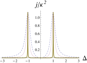
(a)

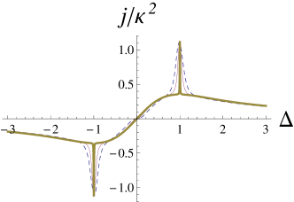
(b)

Figure 3: Typical dependence of renormalized current $j/\kappa^{2}$ versus anisotropy for small driving $\kappa$ and even system size (Panels (a)) and for odd system size, Panel (b). Dashed, thin, and thick lines correspond to $\kappa=0.2,0.1,10^{-2}$ respectively. The system size $N=4$ for Panels (a) and $N=5$ for Panels (b). The curves are given by exact analytic expressions (26) for $N=4$ and analogous analytic expression (not reported) for $N=5$.

The qualitative similarity in the magnetization current behaviour in the cases (i) of weak coupling and large driving, and (ii) weak driving and large coupling is not a trivial one. In the case (ii), the amplitude of the effective $x$- and $y$- boundary gradients is exactly equal to $\kappa$, independently on the anisotropy $\Delta$, so in the limit $\kappa\ll 1$ it becomes infinitesimally small. Also the individual boundary magnetizations $\langle\sigma_{1}^{\alpha}\rangle$,$\langle\sigma_{N}^{\alpha}\rangle$,$\alpha=x,y,z$ are bounded by $\kappa$.

In the case of weak coupling $\Gamma\ll 1$, the amplitude of the boundary gradient at the isotropic point also vanishes in the limit $\Gamma\rightarrow 0$, but the individual boundary magnetizations $\langle\sigma_{1}^{\alpha}\rangle$,$\langle\sigma_{N}^{\alpha}\rangle$ for $\alpha=x,y$ remain finite and are discontinuous at $\Delta=1$.

The presence of the singularity and non-commutativity of the limits $\lim_{\Delta\rightarrow 1}$ and $\lim_{\Gamma\rightarrow 0}$(or $\lim_{\kappa\rightarrow 0}$) must be related to the existence of an additional symmetry which the $XXZ$ model acquires at the isotropic point $\Delta=1$. This symmetry however is not the full rotational symmetry of a unitary quantum $XXX$ Hamiltonian, since the dissipative Lindblad terms in LME do not have the full rotational symmetry. On the other hand, qualitative differences between singularities for odd and even system sizes $N$, seen for spin current, energy current, and other observables, is a consequence of intrinsic properties of the XY-twisted model, which is manifested by (5),(6).

V Conclusions

We have investigated an $XXZ$ spin chain coupled at the ends to a dissipative boundary reservoirs, which impose a twisting angle between the first and the last spin in the $XY$ plane, described by a Lindblad Master equation. We pointed out the non-analytic character of the non-equilibrium steady state in the two limits: of vanishing coupling $\Gamma$ and of vanishing driving $\kappa$. Unlike in the approaches proposed before, where a small but fixed boundary driving (of the order of $10^{-2}$) is being typically used, here we access arbitrary small coupling or driving analytically. Our approach allows to establish a presence of a singularity in the NESS for $\Gamma\rightarrow 0$ and $\kappa\rightarrow 0$, which is expected to be present in the system for all system sizes. The singularity is evidenced on an example of several observables: the magnetization current, the energy current, and the boundary magnetizations. For magnetization current, the analytic treatment is presented.

The character of the singularity qualitatively depends on a parity of system size $N$. For odd $N$ we find that the spin current scales for small $\Gamma$ or small $\kappa$ as $j=f(\Delta)\Gamma^{2},j=g(\Delta)\kappa^{2}$, where for vanishing $\Gamma$ or $\kappa$ the functions $f$ and $g$ have different finite values at $\Delta=1$, and $\Delta=1\pm 0$. For even sizes $N$, the spin current still scales quadratically with $\Gamma$ or $\kappa$ at the point $\Delta=1$, while it scales as $j=f_{1}(\Delta)\Gamma^{4},j=g_{1}(\Delta)\kappa^{4}$ at all other points. The energy current $J^{E}$ scales in the isotropic point linearly with couplings $\Gamma_{L},\Gamma_{R}$ (which must be different, $\Gamma_{L}\neq\Gamma_{R}$), and develops a twin peak singularity. Here we are not already in a position to discuss the conductivity of spin or energy due to the small system sizes; however the DMRG studies ZnidaricJStat2010_2siteLindblad and recently proposed exact approaches might give access to large system sizes and even to the thermodynamic limit.

Acknowledgements VP acknowledges the Dipartimento di Fisica e Astronomia, Università di Firenze, for support through a FIRB initiative. M.S. acknowledges support from the Ministero dell’ Istruzione, dell’ Universitá e della Ricerca (MIUR) through a Programma di Ricerca Scientifica di Rilevante Interesse Nazionale (PRIN)-2010 initiative.

Appendix A Current for $N=5$ (weak driving limit)

For $N=5$ and in the limit $\Gamma\rightarrow\infty$ the exact expression for the current is given by a complicated expression. We report different limits here below. Taking the limit $\lim_{\kappa\rightarrow 0}$ first, we find

$$\lim_{\kappa\rightarrow 0}\frac{j_{0}(\kappa,\Delta)}{\kappa^{2}}=\frac{16\Delta\left(\Delta^{2}+3\right)}{28\Delta^{4}+81\Delta^{2}+72},$$ (30)

and consequently $\lim_{\Delta\rightarrow 1}\lim_{\kappa\rightarrow 0}\frac{j_{0}(\kappa,\Delta)}{\kappa^{2}}=\frac{64}{181}$. On the other hand, taking the limit $\lim_{\Delta\rightarrow 1}$ first, we find $\lim_{\Delta\rightarrow 1}\frac{j_{0}(\kappa,\Delta)}{\kappa^{2}}=-\frac{F}{G}$, where

$$F=8(128\kappa^{22}-2128\kappa^{20}+5792\kappa^{18}+44096\kappa^{16}-245827\kappa^{14}+182930\kappa^{12}+$$

$$980805\kappa^{10}-1523750\kappa^{8}-1515697\kappa^{6}+3477286\kappa^{4}-1171473\kappa^{2}+2235870),$$

$$G=576\kappa^{22}+856\kappa^{20}-34736\kappa^{18}-102787\kappa^{16}+1669223\kappa^{14}-4033065\kappa^{12}-$$

$$2004745\kappa^{10}+13257113\kappa^{8}+3528813\kappa^{6}-16075891\kappa^{4}-7450779\kappa^{2}-15651090$$

and consequently $\lim_{\kappa\rightarrow 0}\lim_{\Delta\rightarrow 1}\frac{j_{0}(\kappa,\Delta)}{\kappa^{2}}=\frac{8}{7}$. Another way to see the discontinuity is to estimate the derivatives $\left.(\partial^{m}j_{0}(\kappa,\Delta)/\partial\kappa^{m})\right|_{\kappa=0}$, all even orders of which, starting from $m=4$, have singularities at $\Delta=1$ as

$$\left.\frac{\partial^{2n}}{\partial\kappa^{2n}}j_{0}(\kappa,\Delta)\right|_{\kappa=0}=O\left(\frac{1}{(\Delta-1)^{2n-2}}\right).$$

For odd $m=2n+1$, we find $\left.(\partial^{2n+1}j_{0}(\kappa,\Delta)/\partial\kappa^{2n+1})\right|_{\kappa=0}=0$.

References

References

- (1) H.-P. Breuer and F. Petruccione, The Theory of Open Quantum Systems, Oxford University Press, (2002).
- (2) M.B. Plenio and P.L Knight, Rev. Mod. Phys. 70, 101 (1998).
- (3) H. Wichterich, M. J. Henrich, H.P. Breuer, J. Gemmer and M. Michel, Phys.Rev. E 76 , 031115 (2007)
- (4) F. Heidrich-Meisner, A. Honecker, and W. Brenig, Eur. Phys. J. Special Topics 151, 135 (2007), and references therein.
- (5) X. Zotos, J. Phys. Soc. Jpn. Supp. 74, 173 (2005) and references therein.
- (6) A. Klumper, Lect. Notes Phys. 645, 349 (2004).
- (7) F. M. D. Haldane, J. Phys. C 14, 2585(1981); A. O. Gogolin and N. V. Prokof’ev, Phys. Rev. B 50, 4921 (1994); Schulz H, 1996, in: “Correlated Fermions and Transport in Mesoscopic Systems”, Les Arcs, Savoie, (Editions Frontieres, 1996)
- (8) U Schollwöck, Rev. Mod. Phys. 77, 259 (2005).
- (9) N. Hlubek, P. Ribeiro, R. Saint-Martin, A. Revcolevschi, G. Roth, G. Behr, B. Büchner, and C. Hess, Phys. Rev. B 81, 020405 (2010).
- (10) T. Prosen and I. Pizorn, Phys. Rev. Lett. 101, 105701 (2008).
- (11) G. Benenti, G. Casati, T. Prosen, D. Rossini and M. Žnidarič, Phys. Rev. B 80, 035110 (2009).
- (12) B. Žunkovič and T. Prosen, J. of Stat. Mech. P08016 (2010).
- (13) T. Prosen, New. J. Phys. 10, 043026 (2008).
- (14) T. Prosen, Phys. Rev. Lett. 107, 137201 (2011).
- (15) D. Karevski, V. Popkov and G. Schütz, Phys. Rev. Lett. 110, 047201 (2013)
- (16) M. Žnidarič, Phys. Rev.Lett. 106, 220601 (2011).
- (17) R. Kubo , M. Toda, N. Hashitsume, Statistical Physics II: Nonequilibrium Statistical Mechanics (Springer Series in Solid-State Sciences)
- (18) V. Popkov, Mario Salerno and G. M. Schütz, Phys. Rev. E 85, 031137 (2012).
- (19) V. Popkov, J. Stat. Mech. (2012) P12015
- (20) V. Popkov and R. Livi, New J. Phys. 15 (2013) 023030
- (21) S. R. Clark, J. Prior, M. J. Hartmann, D. Jaksch and M. B. Plenio, New J. of Phys. 12, 025005(2010).
- (22) M. Salerno and V. Popkov, Phys. Rev. E 87, 022108 (2013)
- (23) The relaxation times depend on spin component. At the left boundary, - and -spin components of relax as while the -spin component relax as , see Lindblad2011
- (24) If , the situation is more subtle since then the target states and are mixed
- (25) For symmetric choice of the couplings (3)the energy current disappears as a consequence of the symmetry (4), see PopkovXYtwist .
- (26) D.E. Evans, Comm. Math. Phys, 54, 293 (1977)
- (27) T. Prosen, Phys. Scr. 86, 058511 (2012).
- (28) T. Prosen and M. Žnidarič, J. Stat. Mech. (2009) P02035; M. Žnidarič, J. of Stat. Mech. P12008 (2011).