Analysis of a combined influence of substrate wetting and surface electromigration on a thin film stability and dynamical morphologies

Abstract

A PDE-based model combining surface electromigration and wetting is developed for the analysis of morphological stability of ultrathin solid films. Adatom mobility is assumed anisotropic, and two directions of the electric field (parallel and perpendicular to the surface) are discussed and contrasted. Linear stability analyses of small-slope evolution equations are performed, followed by computations of fully nonlinear parametric evolution equations that permit surface overhangs. The results reveal parameter domains of instability for wetting and non-wetting films and variable electric field strength, nonlinear steady-state solutions in certain cases, and interesting coarsening behavior for strongly wetting films.

Submitted to the special issue ”Nanoscale wetting of solids on solids” of the journal Comptes Rendus Physique (Olivier Pierre-Louis, Univ. Lyon, Editor)

Keywords: Electromigration ; Wetting ; Dynamics of thin solid films

I Introduction

Since the early 1990’s there has been an interest in understanding and accessing the effects of electromigration on kinetic instabilities of crystal steps St -UCS and epitaxial islands KD -KKHV , and on morphological stability of epitaxial films BMOPL -TGM1 . Among other applications (which were developed primarily at the microscale), electromigration has been also used for fabrication of nanometer-sized gaps in metallic films. Such gaps are suitable for testing of the conductive properties of single molecules and control of their functionalities VFDMSKBM -GSPBT . For instance, Ref. GSPBT describes fabrication of nanoscale contacts by using electromigration to thin down and finally break the epitaxially grown ultrathin (10 ML) Ag films wetting the Si(001) substrate. The gap between contacts can be cyclically opened and closed by applying electromigration current at 80 K to open the gap, and enabling surface diffusion by annealing to the room temperature, to close it.

Thus for this and other emerging applications at the nanoscale WH ; SV it seems important to understand and characterize the effects of substate wetting and electromigration that are simulaneously active in the physical system. This paper combines these effects in a model that is based on an evolution equation(s) for the continuous profile of the film surface. The focus is on wetting films with isotropic surface energy, but with anisotropic adatom mobility KD ; SK , although the model allows any combination of wetting properties and anisotropies. We factor in and discuss the effects on film stability and morphological evolution of the electric field that is either parallel, or perpendicular to the initial planar surface of the film, and do not limit considerations to small deviations from planarity, i.e. the arbitrary surface slopes and even surface overhangs are permitted by the model. Models of wetting appropriate for continuum-level modeling of the surface diffusion-based dynamics of solid films have been developed and discussed extensively primarily in the context of thin film heteroepitaxy CG -K2 . Our analysis is based on one such model, called the two-layer exponential model for the surface energy ORS ; GolovinPRB2004 ; LevinePRB2007 , GillWang -BWA (which is particularly useful when the surface energy is anisotropic), but other models of wetting discussed in Refs. CG -K2 can be used instead, and the results are expected to be qualitatively similar. The goal of modeling in this paper is not to match the theoretical results to the experiment GSPBT and thus help in understanding the experiment, but rather to provide the broad analysis of the interplay of two effects (wetting and electromigration) that, at least to our knowledge, has not been addressed in prior publications.

II Problem Statement

We consider a 2D single-crystal film of unperturbed height $H_{0}$ with the 1D parametric surface
$\Gamma(x(u,t),z(u,t))$, where $x$ and $z$ are the Cartesian coordinates of a point on a surface, $t$ is the time and $u$ is the parameter along the surface. The origin of the Cartesian reference frame is on the substrate, and along the substrate (the $x$-direction) the film is assumed infinite. The $z$-axis is in the direction normal to the substrate and to the initial planar film surface. Surface marker particles will be used for computations of surface dynamics Trygg . Thus $x$ and $z$ ($z>0$) in fact represent the coordinates of a marker particle, which are governed by the two coupled parabolic PDEs Sethian1 ; BKL :

$$x_{t} = Vz_{s}=V\frac{1}{g}z_{u},$$ (1)

$$z_{t} = -Vx_{s}=-V\frac{1}{g}x_{u}.$$ (2)

Here (and below) the subscripts $t,s,u,z$ and $x$ denote partial differentiation with respect to these variables, $V$ is the normal velocity of the surface which incorporates the physics of the problem, and $g(u,t)=s_{u}=z_{u}/\cos{\theta}=\sqrt{x_{u}^{2}+z_{u}^{2}}$. Here $s$ is the surface arclength and $\theta$ the surface orientation angle, i.e. the one that the unit surface normal makes with the reference crystalline direction (chosen along the $z$-axis). If the surface slopes are bounded at all times (surface does not overhang), then it is more convenient to describe surface dynamics by a single evolution PDE for the height function $h(x,t)$ of the film. Eqs. (1), (2) can be easily reduced to such “h-equation”, which we will use for analysis; however, Eqs. (1), (2) will be used for most computations in this paper. Similar parametric approach was used recently in Ref. OL for the computation of a hill-and-valley structure coarsening in the presence of material deposition (growth) and strongly anisotropic surface energy.

Assuming that temperature is sufficiently high and surface diffusion is operative, the normal velocity is given by

$$V=\frac{D\Omega\nu}{kT}\left[\left\{M(\theta)\mu_{s}\right\}_{s}+\alpha E_{0}q\left\{M(\theta)f(\theta)\right\}_{s}\right],$$ (3)

where $D$ is the adatoms diffusivity, $\Omega$ the atomic volume, $\nu$ the adatoms surface density, $kT$ the Boltzmann’s factor, $\mu$ the surface chemical potential, $M(\theta)$ the anisotropic adatom mobility, $E_{0}$ the applied electric field, $q>0$ the effective charge of adatoms, $f(\theta)=\sin{\theta}$, if the electric field is vertical, or $f(\theta)=\cos{\theta}$, if the electric field is horizontal, and $\alpha=\pm 1$ is used to select either stabilizing, or destabilizing action of the field for the chosen combination of the vertical or horizontal orientation of the field and the mobility $M(\theta)$. The two values of $\alpha$ correspond to two possible field orientations once either the horizontal, or the vertical field direction has been chosen (that is, field directed up-down, or left-right). The first term in $V$ describes the high-T surface diffusion, the second term describes surface diffusion enabled by electromigration M .

The surface chemical potential $\mu$ is assumed to have the contributions from the surface energy and the surface wetting interaction with the substrate/film interface:

$$\mu=\Omega\left[\gamma\kappa+\gamma_{z}\cos{\theta}\right],$$ (4)

where $\kappa=\theta_{s}=g^{-3}\left(z_{uu}x_{u}-x_{uu}z_{u}\right)$ is the surface mean curvature and, in the general case, $\gamma(z,\theta)$ is the height- and orientation-dependent, i.e. anisotropic, surface energy. (Note again that $z$ here stands for the shortest distance between the substrate and a chosen point $(x,z)$ on a film surface; this distance is the height $h(x,t)$ of the surface if there is no overhangs.) In this paper we focus on the effects due to anisotropic adatom mobility, thus we will use the simpler isotropic model for the surface energy CG -K2 :

$$\gamma=\gamma(z)=\gamma_{f}+\left(\gamma_{S}-\gamma_{f}\right)\exp{\left(-z/\ell\right)},$$ (5)

where $\gamma_{S}$ is the (constant) energy of a substrate/gas (or vacuum) interface, $\ell$ the characteristic wetting length, and $\gamma_{f}$ the constant energy of a crystal/gas interface (that is, of the film surface). Eq. (5) is the interpolation between the two energies. In the limit of a thick film, $z\rightarrow\infty$, only the latter energy is retained in this expression (because the inter-molecular forces between the substrate and the surface molecules are relatively short-ranged), and in the limit of a film of zero thickness only the former energy is retained. Despite that Eq. (5) is phenomenological, it matches surprisingly well the experiments and the ab-initio calculations (at least for lattice-mismatched systems) GillWang ; WKSM ; BWA .

Finally, we assume the (dimensionless) anisotropic adatom mobility in the form SK

$$M(\theta)=\frac{1+\beta\cos^{2}{[N(\theta+\phi)]}}{1+\beta\cos^{2}{[N\phi]}},$$ (6)

where $N$ is the number of symmetry axes and $\phi$ is the angle between a symmetry direction and the average surface orientation. $\beta$ is a parameter determining the strength of the anisotropy. Throughout the paper we present results either for $\beta=0$ (isotropic case), or for $\beta=1$ and $N=4,\;\phi=\pi/16$. For the latter set of parameters values the graphs of the functions $M(\theta)$ and $M^{\prime}(\theta)$ are shown in Fig. 1.

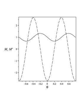
Figure 1: Anisotropic mobility $M(\theta)$ (solid line) and its derivative (dashed line) for $\beta=1,\ N=4$ and $\phi=\pi/16$.

Remark 1. In the limit $z\rightarrow\infty$ (where wetting effect is not operative), the present problem is most closely related to the one analyzed by Schimschak and Krug in Ref. SK . The essential difference is that these authors determine the electric field from the solution of the potential equation with the appropriate boundary conditions on the material boundaries, including the moving surface KAIN ; B . Thus their solution for the electric field is nonlocal, unlike the local approximation used in this paper. The local nature of the electric field explains why we did not detect traveling wave solutions, which are the hallmark of Refs. SK ; B .

Next, we choose $\ell$ as the length scale and $\ell^{2}/D$ as the time scale and write the dimensionless counterparts of Eqs. (1), (2), where we use same notations for dimensionless variables:

$$x_{t} = \left[B\left\{M(\theta)\mu_{s}\right\}_{s}+A\left\{M(\theta)f(\theta)\right\}_{s}\right]z_{s}\equiv Vz_{s},$$ (7)

$$z_{t} = -Vx_{s},$$ (8)

$$\mu = \left[1+(G-1)\exp{(-z)}\right]\kappa+(1-G)\exp{(-z)}\cos{\theta},\;\mbox{where}\;\cos{\theta}=z_{s}.$$ (9)

Notice that the dimensionless forms of $f(\theta)$ and the parametric expression for $\kappa$ coincide with their dimensional forms, and that Eq. (5) has been substituted in Eq. (4). For conciseness, we keep differentiation with respect to the arclength, $s$, in the dimensionless equations, but their most transparent forms for the computations result when the differentiation with respect to $s$ is replaced with the differentiation with respect to the parameter $u$, using $\partial/\partial s=(1/g)\partial/\partial u$. In Eqs. (7) - (9) $B=\Omega^{2}\nu\gamma_{f}/\left(kT\ell^{2}\right)$ is the surface diffusion parameter, $A=\alpha\nu\Omega E_{0}q/(kT)$ is the strength of the electric field, and $G=\gamma_{S}/\gamma_{f}$ is the ratio of substrate to film surface energies. For wetting films $G>1$, for non-wetting films $0<G<1$. Notice that $A$ may take on positive or negative values through the parameter $\alpha$.

As was mentioned above, if there is no overhangs then Eqs. (7)-(9) can be reduced to the single dimensionless evolution equation for the surface height $h$:

$$h_{t}=B\left[M\left(h_{x}\right)\left(1+h_{x}^{2}\right)^{-1/2}\mu_{x}\right]_{x}+A\left[M\left(h_{x}\right)\left(1+h_{x}^{2}\right)^{-1/2}f\left(h_{x}\right)\right]_{x},$$ (10)

where

$$\mu=\left[1+(G-1)\exp{(-h)}\right]\kappa+(1-G)\exp{(-h)}\left(1+h_{x}^{2}\right)^{-1/2},\quad\kappa=-h_{xx}\left(1+h_{x}^{2}\right)^{-3/2},$$ (11)

$f\left(h_{x}\right)=h_{x}$, if the electric field is vertical, or $f\left(h_{x}\right)=1$, if the electric field is horizontal. Also $M\left(h_{x}\right)$ is given by Eq. (6), where $\theta$ is replaced by $arctan\left(h_{x}\right)$.

Using values: $D=1.5\times 10^{-6}$ cm²/s, $\Omega=2\times 10^{-23}$ cm³, $\gamma_{f}=2\times 10^{3}$ erg/cm², $\nu=10^{15}$ cm^-2, $kT=1.12\times 10^{-13}$ erg, $\ell=3\times 10^{-8}$ cm (0.3 nm, or 1ML), gives $B=8$. Using $q=5e$ (where $e=5\times 10^{-10}$ statcoulombs is the absolute value of the electron charge) and the minimum applied voltage difference $\Delta V=5\times 10^{-3}$ Volts acting across the typical distance of the order of the film height, $\Delta L=10$ nm, gives $|qE_{0}|=4\times 10^{-4}$ erg/cm, which translates to $|A|=71$. Applied voltage in surface electromigration experiments at the nanoscale can be as high as 1 V GSPBT , thus in this study we explored the range of field strengths $71\leq|A|\leq 7100$.

In the following sections we analyze several representative situations.

III Vertical electric field

III.1 Linear stability analysis

The small slope approximation $\left(|h_{x}|\ll 1\right)$ of Eq. (10) reads:

$$h_{t}=BM(0)\left[\left\{(1-G)\exp(-h)-1\right\}h_{xxx}+h_{x}(G-1)\exp(-h)\left(h_{xx}+1\right)\right]_{x}+$$

$$\hskip 19.91684ptBM^{\prime}(0)(G-1)\left[\exp(-h)h_{x}^{2}\right]_{x}+AM(0)h_{xx}-\frac{3}{2}AM(0)h_{x}^{2}h_{xx}+2AM^{\prime}(0)h_{x}h_{xx},$$ (12)

where the mobility has been linearized about the flat surface $h_{x}=0$, that is, $M\left(h_{x}\right)=M(0)+M^{\prime}(0)h_{x},\;M(0)>0$. The last two terms are the simplest nonlinearities from the expansion of the electromigration flux that involve $M(0)$ and $M^{\prime}(0)$. Without loss of generality we will take $M(0)=1$ here and elsewhere in this paper. (See Fig. 1. When mobility is isotropic, i.e. $\beta=0$, then $M=M(0)=1$, as is seen from Eq. (6).) Notice that the anisotropy of the mobility, $M^{\prime}(0)$, does not have an effect on linear stability, as it enters in the coefficients of the nonlinear terms. Also note that the last three terms can be written in a conservative form similar to the terms in the first line of the equation and to the first term in the second line (and this is how they are implemented in the code).

Introducing small perturbation $\xi(x,t)$ in Eq. (12) by replacing $h$ with $h_{0}+\xi(x,t)$ (where $h_{0}=H_{0}/\ell$ is the dimensionless unperturbed film height), linearizing in $\xi$ and assuming normal modes for $\xi$, gives the perturbation growth rate $\omega(k)$, where $k$ is the perturbation wavenumber:

$$\omega(k)=-B\left[1+(G-1)\exp(-h_{0})\right]k^{4}-\left[B(G-1)\exp(-h_{0})+A\right]k^{2}.$$ (13)

Remark 2. When wetting interaction is absent (thick film: $h_{0}\rightarrow\infty$), Eq. (13) reduces to the standard one, $\omega(k)=-Bk^{4}-Ak^{2}$, which reflects the stabilizing action of the surface diffusion and either stabilizing ($A>0$, electric field is in the positive $z$ direction), or destabilizing ($A<0$, electric field is in the negative $z$ direction) action of the electric field. Such film is absolutely stable when $A>0$, but when $A<0$ it is long wave-unstable.

III.1.1 Analysis of Eq. (13)

• Wetting films $(G>1)$. From Eq. (13) one notices that wetting films are absolutely linearly stable when $A>0$, but they are long wave-unstable when $A<-B(G-1)\exp(-h_{0})<0$ (see Fig. 2). The short-wavelength cut-off wavenumber, the maximum growth rate, and the wavenumber at which the latter occurs are:

  $$k_{c}=\sqrt{\frac{-A-B(G-1)\exp(-h_{0})}{B[1+(G-1)\exp(-h_{0})]}},\quad\omega_{max}=\frac{1}{4}\frac{\left[A+B(G-1)\exp(-h_{0})\right]^{2}}{B[1+(G-1)\exp(-h_{0})]},\quad k_{max}=\frac{k_{c}}{\sqrt{2}}.$$ (14)

  $k_{c}$ and $\omega_{max}$ are plotted in Figs. 3 and 4. The film stability decreases with increasing $h_{0}$, and this trend saturates around $h_{0}=10$ (3 nm). That is, for the stated field strength $A=-71$ films of thickness $h_{0}>10$ do not ”feel” the stabilizing presence of the substrate, and they are as stable as the films that do not interact with the substrate at all. Of course, increasing field strength $|A|$ makes the film less stable, but increasing $G$ makes it more stable, since the substrate energy provides stabilizing effect. In Figs. 3(c) and 4(c) the rate of decrease of $k_{c}$ and $\omega_{max}$ with $G$ (i.e., the rate of stabilization) increases fast with decreasing $h_{0}$. For $A=-71$ at $h_{0}\sim 3.5$ and $G\sim 300$ the entire dispersion curve $\omega(k)$ is below the $k$-axis, see the dashed curves in Figs. 3(c) and 4(c), and thus the film is absolutely linearly stable for $h_{0}<\sim 3.5$ and $G>\sim 300$. By analysing the condition for longwave instability, $A<-B(G-1)\exp(-h_{0})<0$, one can get an understanding of why this happens.

  

  Figure 2: Sketch of perturbation’s linear growth rate $\omega(k)$ corresponding to longwave instability of the film surface.

  

  

  

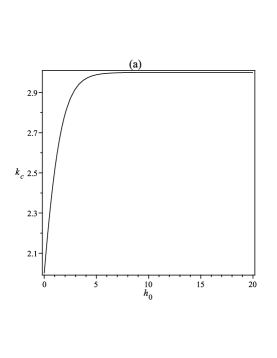
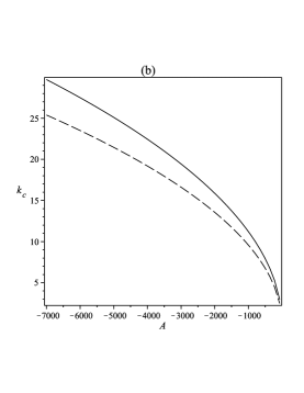
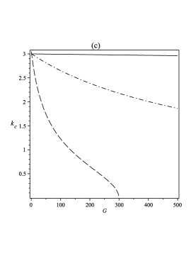
  Figure 3: Wetting films and vertical electric field: Instability cut-off wavenumber $k_{c}$. (a) vs. $h_{0}$, $A=-71,\ G=2$; (b) vs. $A$, $h_{0}=10$ (solid line), $h_{0}=1$ (dashed line). $G=2$; (c) vs. $G$, $h_{0}=10$ (solid line), $h_{0}=6$ (dash-dotted line), $h_{0}=3.5$ (dashed line). $A=-71$.

  

  

  

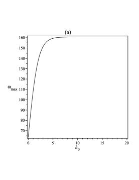
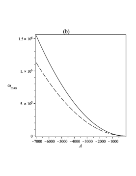
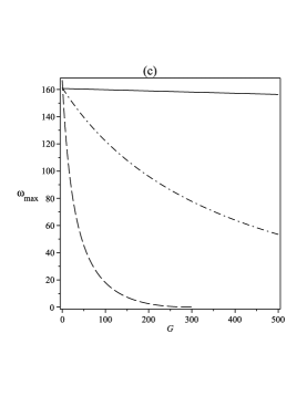
  Figure 4: Wetting films and vertical electric field: Maximum growth rate $\omega$. Cases (a)-(c) are as in Fig. 3.

  Indeed, this condition is equivalent to $h_{0}>\ln{\left(BA^{-1}(1-G)\right)}$, and for the typical values of $A$ and $B$ stated above and for moderately large $G$ the right-hand side of the latter inequality is negative, thus the longwave instability occurs for any film height $h_{0}$. This is similar to the situation when wetting effects are absent, see Remark 2 (but of course the spectrum of unstable wavenumbers and the magnitude of the maximum growth rate are different). There is a critical thickness $h_{0c}$ below which the film is absolutely linearly stable only if $G-1\sim|A|$, i.e. when $G$ is of the order of at least one hundred.

• Non-wetting films $(0<G<1)$. In this case, for $A<0$ the long-wave instability occurs for any film thickness and any electric field strength - which is again similar to the situation when wetting effects are absent, see Remark 2. When $A>0$ the long-wave instability (with $k_{c},\;\omega_{max}$ and $k_{max}$ numerically similar to those shown in Eq. (14)) occurs when the film height is less than critical, $h_{0}<h_{0c}=\ln{\left(AB^{-1}(1-G)^{-1}\right)}$. When $h_{0}>h_{0c}$ the film is absolutely linearly stable. $h_{0c}$ is plotted in Fig. 5. It is clear that $h_{0c}$ increases with increasing either $A$, or $G$, or both parameters.

  

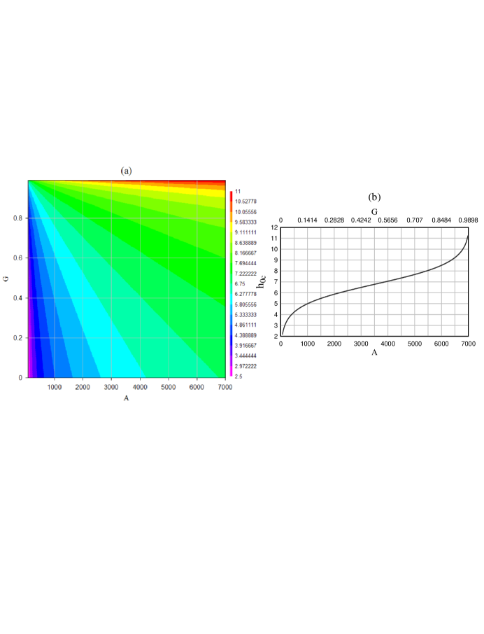
  Figure 5: (Color online). Non-wetting films and vertical electric field: (a) Contour plot of the critical thickness $h_{0c}$. (b) Diagonal cross-section (from the lower left corner to the upper right corner) of the contour plot in (a).

III.2 Nonlinear surface dynamics of wetting films

Computations with the small-slope Eq. (12) (where $M(0)=1,\;M^{\prime}(0)=0$) were performed for $G=2$ and varying field strengths $A$ that satisfy the condition for long-wave instability, $A<-B(G-1)\exp(-h_{0})<0$. Computational domain was $0\leq x\leq\lambda_{max},\;\lambda_{max}=2\pi/k_{max}$ with periodic boundary conditions, and the initial condition was the small-amplitude cosine-shaped perturbation of the flat surface $h_{0}=const.$ All computations produced steady-state solutions that have the shape of a vertically stretched cosine curve with a fairly large amplitude. However, neither of these steady-states were confirmed when instead fully nonlinear parametric equations (7) - (9) were computed. Fig. 6 shows the computed morphology. Overhangs are clearly visible, and the bottom of the ”pit” flattens out as it approaches the substrate due to increase of the repulsive force, promoting overhangs in the vicinity.

Similarly, when Eq. (12) was computed with the random small-amplitude initial condition on the domain $0\leq x\leq 20\lambda_{max}$ (the mobility was again isotropic), the result was a perpetually coarsening hill-and-valley structure. This was again not confirmed in the computations of parametric equations. The late time morphology computed using the parametric equations is shown in Fig. 7(a). The surface develops deep “pockets” whose walls overhang and eventually merge, resulting in tear drop-shaped voids trapped in the solid; this can be seen, for instance, on the interval $40<x<50$. Fig. 7(b) shows the typical random initial condition.

Anisotropic mobility resulted in morphologies that are similar to ones shown in Figs. 6 and 7(a), but skewed left or right, depending on the sign of $\phi$. As we pointed in Sec. III.1, anisotropy matters in the nonlinear stage of the dynamics.

Figure 6: Wetting films, vertical electric field, isotropic mobility: One wavelength of the surface morphology on the periodic domain $0\leq x\leq\lambda_{max}$, computed using Eq. (12) ($M^{\prime}(0)=0$) starting from the small-amplitude cosine-shaped initial condition. $A=-71,\ h_{0}=10,\ G=2$.

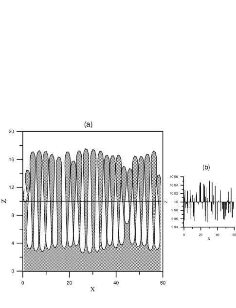
Figure 7: Wetting films, vertical electric field, isotropic mobility: (a) Surface morphology computed using Eqs. (7) - (9) ($\beta=0$ in Eq. (6)) on the domain $0\leq x\leq 20\lambda_{max}$, starting from the small-amplitude random initial condition shown in (b). $A=-71,\ h_{0}=10,\ G=2$.

IV Horizontal electric field

IV.1 Linear stability analysis

In the case of the horizontal electric field the small slope approximation of Eq. (10) reads:

$$h_{t}=B\left[\left\{(1-G)\exp(-h)-1\right\}h_{xxx}+h_{x}(G-1)\exp(-h)\left(h_{xx}+1\right)\right]_{x}+$$

$$\hskip 19.91684ptBM^{\prime}(0)(G-1)\left[\exp(-h)h_{x}^{2}\right]_{x}-Ah_{x}h_{xx}+AM^{\prime}(0)h_{xx}-\frac{3}{2}AM^{\prime}(0)h_{x}^{2}h_{xx}.$$ (15)

Again here we retained two simplest nonlinearities from the expansion of the electromigration flux term. The coefficient $M(0)$ in the third-to-last term has been set equal to one. This nonlinear term and the last (nonlinear) term in Eq. (15) do not have an effect on linear stability. Unless mobility is isotropic, the second-to-last term of Eq. (15) has an effect on linear stability. Assuming anisotropy, the growth rate is

$$\omega(k)=-B\left[1+(G-1)\exp(-h_{0})\right]k^{4}-\left[B(G-1)\exp(-h_{0})+AM^{\prime}(0)\right]k^{2}.$$ (16)

Comparing Eqs. (13) and (16), it is clear that one can obtain stability properties in the horizontal field case by replacing $A$ in Eq. (13) with $AM^{\prime}(0)$. Since $M^{\prime}(0)\approx-2.7$ (see Fig. 1) for the chosen parameter values in Eq. (6), then for instability one must have $A>0$ (the electric field is in the positive $x$ direction). Thus, for instance, the stability analysis of wetting films in the paragraph 1. of Sec. III.1.1 translates directly into the case of the horizontal field simply by replacing $A$ in the formulas by $-2.7A$, where $A>0$. Figs. 3(b) and 4(b) are also valid in the case of the horizontal field if the $A$ values along the horizontal axes are understood as values of the product $-2.7A$ (thus the absolute characteristic $A$ values are roughly three times smaller than in the case of the vertical field).

IV.2 Nonlinear surface dynamics of wetting films

IV.2.1 Periodic steady-states from sinusoidal perturbations

Computations with either the small-slope Eq. (15), or the parametric equations (7)-(9), of the evolution of a one wavelength ($\lambda$), small-amplitude cosine curve-shaped perturbation on a periodic domain resulted in steady-state profiles which have a shape of a vertically stretched cosine curve with a fairly large amplitude. The steady-state profiles often displayed a more sharply peaked bottom and less curved walls than the cosine curve, and the amplitude is significantly smaller in the (fully nonlinear) parametric case. In fact, it can be noticed from Fig. 8 that the film is nowhere close to dewetting the substrate for all tested field strengths, notwithstanding that the stabilizing influence of the substrate is minimal for the chosen parameters values (see the discussion in Sections III.1.1, paragraph 1, and IV.1).

Remark 3. When Eq. (15) is used in a computation, the last term there is at large responsible for the saturation of the surface slope and the existence of the steady state. When this nonlinear term is omitted from the equation, the slope increases until the computation breaks down.

In the computations of the parametric equations, unless $\lambda$ is larger than approximately $4\lambda_{max}$, the surface evolves towards the steady-state mostly by vertical stretching of the initial shape. Perturbations of larger wavelength develop a large-amplitude, hill-and-valley type distortions which slowly coarsen into a steady-state, cosine curve-type shape. Fig. 8 shows the amplitude of the steady-state profile, $h_{max}-h_{min}$, and the height of the profile at it’s lowest point, $h_{min}$, vs. $\lambda$.

Figure 8: Wetting films, horizontal electric field, anisotropic mobility: Amplitude of the steady state vs. the perturbation wavelength $\lambda$ for different strengths of the electric field. Upper inset - zoom into the area of the graph around $\lambda=0.5$. Lower inset - minimum height of the steady state profile vs. $\lambda$, also for different strengths of the electric field. Arrows labeled “$\lambda_{max}$” point out the $\lambda_{max}$ value for each of the three electric field strengths. Parameters values are $h_{0}=10,\ G=2$.

It can be seen that, at least for moderate strengths of the electric field, growth of the amplitude is logarithmic in the vicinity of $\lambda_{c}$, and for $\lambda\gg\lambda_{c}$ growth is linear. The numerically determined slope of the linear section of $A=71$ curve is 0.208, the one of the $A=710$ curve is 0.217, and the one of the $A=7100$ curve is 0.209, which suggests that the slope is insensitive (or very weakly sensitive) to the field strength. The decay of $h_{min}$ with increasing wavelength mirrors the growth of the amplitude, thus the steady-state surface shape is symmetrically vertically stretched about the equilibrium surface position $h_{0}=10$. All computed steady-states are stable with respect to imposition of random small- and large-amplitude point perturbations, which we confirmed by computing the dynamics of such perturbed shapes.

IV.2.2 Coarsening of random initial roughness

We employed fully nonlinear simulations based on parametric equations for determination of the coarsening laws at increasing electric field strength and at variable wetting strength (characterized by values of the parameters $h_{0}$ and $G$). Computations were performed on the domain $0\leq x\leq 20\lambda_{max}$ with periodic boundary conditions; all runs were terminated after the surface evolved into a large-amplitude hill-and-valley structure with 3-5 hills. Unless wetting is strong, i.e. $h_{0}$ is small and $G$ is large - the case that is discussed in more detail below - the slopes of the hills are constant 24^∘ during coarsening, except for the short initial period. Figs. 9 - 11 are the log-log plots of the averaged, over ten realizations, maximum surface amplitude $h_{max}-h_{min}$ and the averaged mean horizontal distance $X$ between valleys (kinks) vs. time.

Remark 4. We also attempted to compute coarsening dynamics resulting from the small-slope Eq. (15). While the hill-and-valley structure does emerge and coarsens with time, the characteristic constant hill slope is nearly 90^∘. This suggests that additional nonlinear terms must be retained in Eq. (15) for predictive computations and raises the question what terms must be retained. We had not tried to obtain an adequate nonlinear small-slope model, leaving this agenda to future research.

Of course, increasing the field strength results in faster coarsening, as the times needed for coarsening into a “final” structure are $10^{3}$, $10$, and $1$ for field strengths $A=71,\ 710$ and $7100$, respectively. These values also point out the decrease of the rate of change of a coarsening rate with the increasing field strength. Other than that, the coarsening laws are similar for the three tested field strengths. Fits to the data in the case $A=71$ are shown in Figs. 9(a,b). At small times coarsening is fast (exponential, see Fig. 9(b)), then it changes to a slower power law with the exponent in the range $\sim 0.1\div 0.2$. (Since the values of the amplitude’s logarithm are negative, we were unable to fit the exponential law to the data in Fig. 9(a), thus we fitted the quadratic, which results in the $t^{\epsilon_{1}+\epsilon_{2}\log_{10}t}$-type law.)

Remarkably, when $h_{0}$ is decreased from 10 to 6 a very different coarsening behaviors emerge, see Figs. 10(a,b) and 11(a,b). At $G=2$, after the period of slow power-law coarsening at intermediate times, the coarsening accelerates to exponential coarsening or $t^{\epsilon_{1}+\epsilon_{2}\log_{10}t}$ type coarsening at late times (Figs. 10(a,b)). (For reference, the linear stability in the case $h_{0}=6$ is shown in Figs. 3(c) and 4(c) by the dash-dotted line.) At $G=500$ we did not output a sufficient number of data points in the beginning of the computation, but it is expected that initial coarsening is still faster than the power law. The amplitude starts to decrease towards the end of the simulation, and the kink-kink distance coarsens fast on the entire time interval.

It seems certain that such unusual dynamics in the strongly wetting states emerges due to nonlinear ”overdamping” of electromigration-induced faceting instability by the surface-substrate interaction force. Toward this end, in Figs. 12(a,b) the surface shapes and surface slopes for $h_{0}=10,\ G=2$ and $h_{0}=6,\ G=500$ cases are compared at the time when seven hills formed on the surface. In the former case the hills are steep, have rather uniform height and their slopes are almost straight lines. In the latter case they are more irregular, ”rounded”, and the average height is smaller. It is reasonable to expect that in the opposite case of non-wetting films, the surface-substrate interaction will instead “sharpen up” the hills, i.e. increase their slopes and make the surface structures appear more spatially and temporally uniform.

Finally, we remark that the discussed coarsening laws for strong wetting cases also are qualitatively different from the laws governing coarsening in the absence of wetting, but in the presence of deposition, attachment-detachment, strong surface energy anisotropy, and interface kinetics OL ; SGDNV . Indeed, only the coarsening exponents shown in Fig. 9 (week wetting) are within the same range (0.1-0.5) for nearly the whole computational time interval, as are the exponents computed in the cited papers.

Figure 9: Wetting films, horizontal electric field, anisotropic mobility: (a) Log-log plot of the averaged (over ten realizations) maximum hill height; (b) Log-log plot of averaged kink-kink (valley-valley) distance. Dots: computed data, lines: fitting curves. $A=71,\ h_{0}=10,\ G=2$.

Figure 10: Same as Fig. 9, for $A=71,\ h_{0}=6,\ G=2$.

Figure 11: Same as Figs. 9 and 10, for $A=71,\ h_{0}=6,\ G=500$.

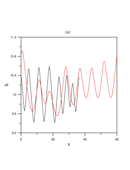
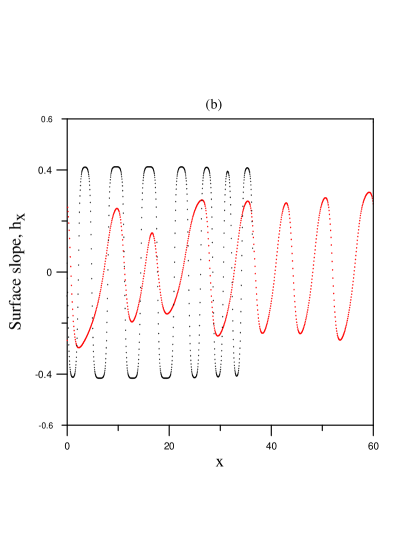
Figure 12: (Color online.) Wetting films, horizontal electric field, anisotropic mobility: (a) Surface height. Black line: $A=71,\ h_{0}=10,\ G=2$, red line: $A=71,\ h_{0}=6,\ G=500$; (b) Surface slope. Black crosses: $A=71,\ h_{0}=10,\ G=2$, red triangles: $A=71,\ h_{0}=6,\ G=500$. Note that the computational domains are of different length for the two presented cases, since the $\lambda_{max}$ values differ.

V Conclusions

In this paper the effects of electromigration and wetting on thin film morphologies are discussed, based on the continuum model of film surface dynamics. It has been shown that wetting effect modifies significantly the stability properties of the film and the coarsening of electromigration-induced surface roughness. Also it has been shown that the small-slope evolution equations that were employed in many studies of electromigration effects on surfaces, are often inadequate for the description of strongly-nonlinear phases of the dynamics. It is expected that the account of the surface energy anisotropy and the electric field non-locality (through the solution of the moving boundary value problem for the electric potential) will lead to uncovering of even more complicated behaviours.

References

- (1) S. Stoyanov, “Current-induced step bunching at vicinal surfaces during crystal sublimation”, Surf. Sci. 370, 345 (1997).
- (2) D.J. Liu, J.D. Weeks, and D. Kandel, “Current-induced step bending instability on vicinal surfaces”, Phys. Rev. Lett. 81, 2743 (1998).
- (3) M. Dufay, J.-M. Debierre, and T. Frisch, “Electromigration-induced step meandering on vicinal surfaces: Nonlinear evolution equation”, Phys. Rev. B 75, 045413 (2007).
- (4) J. Chang, O. Pierre-Louis, and C. Misbah, “Birth and morphological evolution of step bunches under electromigration”, Phys. Rev. Lett. 96, 195901 (2006).
- (5) O. Pierre-Louis, “Local electromigration model for crystal surfaces”, Phys. Rev. Lett. 96, 135901 (2006).
- (6) J. Quah and D. Margetis, “Electromigration in macroscopic relaxation of stepped surfaces”, Multiscale Model. and Simul. 8, 667 (2010).
- (7) V. Usov, C.O. Coileain, and I.V. Shvets, “Influence of electromigration field on the step bunching process on Si(111)”, Phys. Rev. B 82, 153301 (2010).
- (8) J. Krug and H.T. Dobbs, “Current-induced faceting of crystal surfaces”, Phys. Rev. Lett. 73, 1947 (1994).
- (9) M. Schimschak and J. Krug, “Surface electromigration as a moving boundary value problem”, Phys. Rev. Lett. 78, 278 (1997).
- (10) F. Hausser, S. Rasche, and A. Voigt, “The influence of electric fields on nanostructures-simulation and control”, Math. Comput. Simul. 80, 1449-1457 (2010).
- (11) O. Pierre-Louis and T.L. Einstein, “Electromigration of single layer clusters”, Phys. Rev. B 62, 13697 (2000).
- (12) F. Hausser, P. Kuhn J. Krug and A. Voigt, “Morphological stability of electromigration-driven vacancy islands”, Phys. Rev. E 75, 046210 (2007).
- (13) P. Kuhn, J. Krug, F. Hausser, and A. Voigt, “Complex shape evolution of electromigration-driven single-layer islands”, Phys. Rev. Lett. 94, 166105 (2005).
- (14) F. Barakat, K. Martens, and O. Pierre-Louis, “Nonlinear wavelength selection in surface faceting under electromigration”, Phys. Rev. Lett. 109, 056101 (2012).
- (15) D. Maroudas, “Surface morphological response of crystalline solids to mechanical stresses and electric fields”, Surf. Sci. Reports 66, 299-346 (2011).
- (16) V. Tomar, M.R. Gungor, and D. Maroudas, “Current-induced stabilization of surface morphology in stressed solids”, Phys. Rev. Lett. 100, 036106 (2008).
- (17) L. Valladares, L.L. Felix, A.B. Dominguez, T. Mitrelias, F. Sfigakis, S.I. Khondaker, C.H.W. Barnes, and Y. Majima, “Controlled electroplating and electromigration in nickel electrodes for nanogap formation”, Nanotechnology 21, 445304 (2010).
- (18) T. Taychatanapat, K.I. Bolotin, F. Kuemmeth, and D.C. Ralph, “Imaging electromigration during the formation of break junctions”, Nano Lett. 7, 652-656 (2007).
- (19) G. Gardinowski, J. Schmeidel, H. Phnur, T. Block, and C. Tegenkamp, “Switchable nanometer contacts: Ultrathin Ag nanostructures on Si(100)”, Appl. Phys. Lett. 89, 063120 (2006).
- (20) Z.-J. Wu and P.S. Ho, “Size effect on the electron wind force for electromigration at the top metal-dielectric interface in nanoscale interconnects”, Appl. Phys. Lett. 101, 101601 (2012).
- (21) D. Solenov and K.A. Velizhanin, “Adsorbate transport on graphene by electromigration”, Phys. Rev. Lett. 109, 095504 (2012).
- (22) C.-H. Chiu and H. Gao, in: S.P. Baker et al. (Eds.), Thin Films: Stresses and Mechanical Properties V, MRS Symposia Proceedings, vol. 356, Materials Research Society, Pittsburgh, 1995, p. 33.
- (23) Z. Suo and Z. Zhang, “Epitaxial films stabilized by long-range forces”, Phys. Rev. B 58, 5116 (1998).
- (24) M. Ortiz, E.A. Repetto, and H. Si, “A continuum model of kinetic roughening and coarsening in thin films”, J. Mech. Phys. Solids 47, 697 (1999).
- (25) Ya-Pu Zhao, “Morphological stability of epitaxial thin elastic films by van der Waals force”, Arch. Appl. Mech. 72, 77-84 (2002).
- (26) J.-N. Aqua, T. Frisch, and A. Verga, “Ordering of strained islands during surface growth”, Phys. Rev. E 81, 021605 (2010).
- (27) T.O. Ogurtani, A. Celik, and E.E. Oren, “Morphological evolution in a strained-heteroepitaxial solid droplet on a rigid substrate: Dynamical simulations”, J. Appl. Phys. 108, 063527 (2010).
- (28) A.A. Golovin, M.S. Levine, T.V. Savina, and S.H. Davis, “Faceting instability in the presence of wetting interactions: A mechanism for the formation of quantum dots ”, Phys. Rev. B 70, 235342 (2004).
- (29) M.S. Levine, A.A. Golovin, S.H. Davis, and P.W. Voorhees, “Self-assembly of quantum dots in a thin epitaxial film wetting an elastic substrate”, Phys. Rev. B 75, 205312 (2007).
- (30) Y. Pang and R. Huang, “Nonlinear effect of stress and wetting on surface evolution of epitaxial thin films”, Phys. Rev. B 74, 075413 (2006).
- (31) B.J. Spencer, “Asymptotic derivation of the glued-wetting-layer model and contact-angle condition for Stranski-Krastanow islands”, Phys. Rev. B 59, 2011 (1999).
- (32) S.P.A. Gill and T. Wang, “On the existence of a critical perturbation amplitude for the Stranski-Krastanov transition”, Surf. Sci. 602, 3560 (2008).
- (33) M. Khenner, W.T. Tekalign, and M. Levine, “Stability of a strongly anisotropic thin epitaxial film in a wetting interaction with elastic substrate”, Eur. Phys. Lett. 93, 26001 (2011).
- (34) M. Khenner, “Comparative study of a solid film dewetting in an attractive substrate potentials with the exponential and the algebraic decay”, Math. Model. Nat. Phenom. 3, 16-29 (2008).
- (35) M. Khenner, “Morphologies and kinetics of a dewetting ultrathin solid film”, Phys. Rev. B 77, 245445 (2008).
- (36) L.G. Wang, P. Kratzer, M. Scheffler, and N. Moll, “Formation and stability of self-assembled coherent islands in highly mismatched heteroepitaxy”, Phys. Rev. Lett. 82, 4042 (1999).
- (37) M.J. Beck, A. van de Walle, and M. Asta, “Surface energetics and structure of the Ge wetting layer on Si(100)”, Phys. Rev. B 70, 205337 (2004).
- (38) G. Tryggvason, B. Bunner, A. Esmaeeli, D. Juric, N. Al-Rawahi, W. Tauber, J. Han, S. Nas, and Y.-J. Jan, “A front-tracking method for the computations of multiphase flow”, J. Comput. Phys. 169, 708 (2001).
- (39) J.A. Sethian, “A review of recent numerical algorithms for hypersurfaces moving with curvature-dependent speed”, J. Diff. Geom. 31, 131 (1990).
- (40) R.C. Brower, D.A. Kessler, J. Koplik, and H. Levine, “ Geometrical models of interface evolution”, Phys. Rev. A 29, 1335-1342 (1984).
- (41) C. Ograin and J. Lowengrub, “Geometric evolution law for modeling strongly anisotropic thin-film morphology”, Phys. Rev. E 84, 061606 (2011).
- (42) W.W. Mullins, “Solid surface morphologies governed by capillarity”, in Metal Surfaces: Structure, Energetics and Kinetics, 17-66 (1963) (American Society for Metals, Cleveland, OH).
- (43) M. Khenner, A. Averbuch, M. Israeli, and M. Nathan, “Numerical simulation of grain boundary grooving by level set method”, J. Comp. Phys. 170, 764 (2001).
- (44) R.M. Bradley, “Electromigration-induced propagation of nonlinear surface waves”, Phys. Rev. E 65, 036603 (2002).
- (45) T.V. Savina, A.A. Golovin, S.H. Davis, A.A. Nepomnyashchy, and P.W. Voorhees, “Faceting of a growing crystal surface by surface diffusion”, Phys. Rev. E 67, 021606 (2003).