Radiative cooling in collisionally and photo ionized plasmas

Abstract

We discuss recent improvements in the calculation of the radiative cooling in both collisionally and photo ionized plasmas. We are extending the spectral simulation code Cloudy so that as much as possible of the underlying atomic data is taken from external databases, some created by others, some developed by the Cloudy team. This paper focuses on recent changes in the treatment of many stages of ionization of iron, and discusses its extensions to other elements. The H-like and He-like ions are treated in the iso-electronic approach described previously. Fe ii is a special case treated with a large model atom. Here we focus on Fe iii through Fe xxiv, ions which are important contributors to the radiative cooling of hot ($T\sim 10^{5}-10^{7}{\rm\thinspace K}$) plasmas and for X-ray spectroscopy. We use the Chianti atomic database to greatly expand the number of transitions in the cooling function. Chianti only includes lines that have atomic data computed by sophisticated methods. This limits the line list to lower excitation, longer wavelength, transitions. We had previously included lines from the Opacity Project database, which tends to include higher energy, shorter wavelength, transitions. These were combined with various forms of the “g-bar” approximation, a highly approximate method of estimating collision rates. For several iron ions the two databases are almost entirely complementary. We adopt a hybrid approach in which we use Chianti where possible, supplemented by lines from the Opacity Project for shorter wavelength transitions. The total cooling including the lightest thirty element differs from some previous calculations by significant amounts.

1 Introduction

This paper describes recent advances in the treatment of cooling in the spectral simulation code Cloudy. The companion paper, Williams et al. (in preparation), determines the emission spectrum of a non-equilibrium cooling and recombining plasma where the physics is largely driven by radiative cooling.

Cloudy performs, as its primary goal, a full simulation of the microphysics of a non-equilibrium gas. As described in the last major review, (Ferland et al., 1998), the code is designed to incorporate the essential microphysics of gas between the molecular and fully ionized limits, with densities between LTE and the low-density limit, and with temperatures between the current CMB and $10^{10}{\rm\thinspace K}$. Osterbrock & Ferland (2006), hereafter AGN3, provides many details of this physics. Our approach is to treat the microphysics in great detail, using basic cross sections and transition rates where possible, to do exactly what nature does under this broad range of conditions.

The atomic / molecular database is the essential difficulty in producing a full simulation of a non-equilibrium gas. Atomic data, like the underlying quantum mechanics, is complex due to the idiosyncrasies that are characteristic of each molecule or ion. Through much of its history we have added physical processes to the code as special cases, each treated individually. A large model of the Fe ii atom was developed by Katya Verner as part of her PhD thesis (Verner et al., 1999), while Gargi Shaw did a complete model of the hydrogen molecule as part of her PhD thesis (Shaw et al., 2005). Ryan Porter developed a unified treatment of the He-like iso-sequence [Porter et al. (2005) and Porter & Ferland (2007)] and extended it to include the H-like sequence (Luridiana et al., 2009) as part of his thesis.

Additional contributors to the emission spectrum and cooling were added on a line by line basis. Initially a range of lines based on previous calculations of the cooling function were used (Kato (1976); Gaetz & Salpeter (1983)). Additional lines were added on an ad hoc basis. Finally, all Opacity Project (Seaton, 1987) permitted lines that directly connect to the ground state were added (see also Verner et al. (1996)). The Opacity Project did not compute collision rates so the emission data were combined with various forms of the “g-bar” approximation, an approximate relationship between the collision rate and other atomic parameters, to compute the emission. The current implementation uses g-bar approximations from Mewe (1972), Gaetz & Salpeter (1983), and Mewe et al. (1985). Additionally, level energies and line wavelengths for OP lines are uncertain by roughly 15%, although these energies can be removed by comparing with experiments, as was done by Verner et al. (1996). The new improvements are described next.

2 Calculations

We have updated Cloudy to use iron lines from the Chianti database (Dere et al. (1997); Landi et al. (2012)) version 7. Of the astrophysically abundant elements, iron is the one with the richest spectrum and an element which has been an emphasis for the Chianti project. Cloudy will now make use of the experimentally measured lines from the Chianti database for Fe iv through Fe xxiv. The Chianti implementations of Fe xxv and Fe xxvi, He-like and H-like iron, are not used because we treat these using the iso-electronic approach described in Porter et al. (2005), Porter & Ferland (2007), and Luridiana et al. (2009). The special case of Fe ii continues to be treated with the Verner model atom.

In situations where Chianti has provided transitions without collision strengths, the g-bar approximation from Mewe (1972) is used. The transitions are estimated to be allowed or forbidden based on their oscillator strengths values ($gf$). Transitions where $gf\geq 1\times 10^{-8}$ are classified as allowed, all others are forbidden. After classification the appropriate g-bar approximation equation is used.

In addition to the Chianti database lines for Fe iv through Fe xxiv, we added Fe iii lines from the Kurucz Atomic Database (Kurucz, 2009). The Kurucz lines, like the Opacity Project lines, lack collisional data so we use the g-bar approximation. We will use the Chianti and Kurucz data where they are available since they have more accurate energies. We supplement these with Opacity Project lines that come from levels that have higher excitation than those in Chianti and Kurucz. This implementation, called the Hybrid configuration, gives Cloudy the greatest accuracy and wavelength coverage.

In remainder of this section we outline our approach and compute cooling functions for collisionally and photo ionized plasmas. We find surprisingly good agreement with older calculations, and with others based on a detailed incorporation of the atomic physics, but not with several recent studies.

A calculation of the gas cooling involves several steps. First the ionization or chemical state of the gas must be determined. This distribution is then used to compute the cooling, the rate that collisions convert kinetic energy into light. The following sections give details concerning these calculations.

2.1 The ionization balance

This paper is limited to atomic and ionic cooling, and so is limited to temperatures greater than $10^{4}$ K. A calculation of the ionization balance involves rates for collisional and photo ionization, and various recombination processes. These are described in the following subsections.

2.1.1 Collisional Ionization

Cloudy has used the collisional ionization rate coefficients tabulated by Voronov (1997) since soon after the publication of that paper. More recently Dere (2007) presented a new compilation which is largely in excellent agreement with Voronov (1997). The Dere (2007) recommendations originated with experiments from different sources and theoretical calculations using the Flexible Atomic Code (FAC) described in Gu (2002). The collisional ionization rate coefficients of Dere (2007) and Voronov (1997) only differ significantly for about half a dozen ions. We provided options which will allow Cloudy to use either set of rates.

We have implemented these data in the following way in our default calculation. The Dere (2007) coefficients are provided in a discrete format for selected temperatures which do not span the temperature range needed by Cloudy. Voronov (1997) provides continuous functions which are valid for any temperature, going to the appropriate low and high temperature limits. We scaled the Voronov (1997) rates to the values of Dere (2007). For each species, the scale factor is the ratio of the Dere (2007) to Voronov (1997) rates at the center of the temperature range where the ion abundance peaks. These scaling coefficients are typically within 10% of unity. This is now the default for Cloudy.

Table 1: Log of fractional ionization of hydrogen and helium. See the online version of this table which includes the 30 lightest elements and has higher temperature resolution.

$T_{e}(K)$	H0	H+	He0	He+	He2+
4	0.00	-3.34	0.00	–	–
4.5	-2.56	0.00	-0.55	-0.15	-5.71
5	-4.71	0.00	-4.15	-0.95	-0.05
5.5	-5.84	0.00	-7.17	-3.35	0.00
6	-6.59	0.00	–	-4.53	0.00
6.5	-7.16	0.00	–	-5.30	0.00
7	-7.68	0.00	–	-5.89	0.00
7.5	-8.18	0.00	–	-6.43	0.00
8	-8.70	0.00	–	-6.98	0.00
8.5	–	0.00	–	-7.55	0.00
9	–	0.00	–	-8.14	0.00

2.1.2 Photoionization

The photoionization cross section database remains unchanged from Ferland et al. (1998).

2.1.3 Recombination coefficients

We updated Cloudy with the latest radiative (RR) and dielectronic recombination (DR) rate coefficients from Badnell’s website (Badnell et al. (2003) and Badnell (2006)). The update to the DR rate coefficients includes recent data for the argon-like isoelectronic sequence (Nikolić et al., 2010) and Abdel-Naby et al. (2012) for the aluminium-like sequence. We use an ion-specific “mean” value for species which are not covered by the Badnell database, as was described by Ali et al. (1991).

2.2 Temperatures of peak abundance for photoionization and collisional ionization

Our goal is to simulate both photo and collisionally ionized plasmas, for a wide range of chemical abundances and energy sources. There are two limiting cases that are considered in much of the active literature. In the photoionization case the gas is irradiated by an external energy source and the equations of thermal and ionization equilibrium are solved (Osterbrock & Ferland, 2006). The gas kinetic temperature will depend on both the spectral energy distribution (SED) and the composition, being higher for harder SEDs or lower abundances. The ionization distribution is set by the balance between photoionization and recombination rates, and is not directly set by the kinetic temperature. Similarly, the cooling is not a unique function of the temperature in this case. In the collisional ionization case the gas kinetic temperature is often specified, having been set by physics external to the problem, although it would be possible to specify a heating rate and determine the temperature. The ionization distribution is set by the balance between collisional ionization and recombination rates. The ionization and cooling are directly determined by the temperature in this collisional case.

The temperature where a particular ion reaches it peak abundance is different for these two cases. We computed a series of models using solar abundances and a density of $1{\rm\thinspace cm^{-3}}$. Given these assumptions the gas ionization, for an optically thin cell, depends on the gas temperature in the collisional case, and on the intensity of light striking the gas in the photoionization case. The “ionization parameter”, a way of specifying the intensity of the radiation field, was varied in the photoionization case and the Mathews & Ferland (1987) SED of a typical Active Galactic Nucleus was used. In the collisional case the kinetic temperature was varied and the ionization balance determined. The temperature where each successive iron ion peaked was then determined, and is plotted in Figure 1. Figure 1 shows that for a given iron ion, the temperature of peak abundance is significantly higher when collisions rather than photons dominate ionizations.

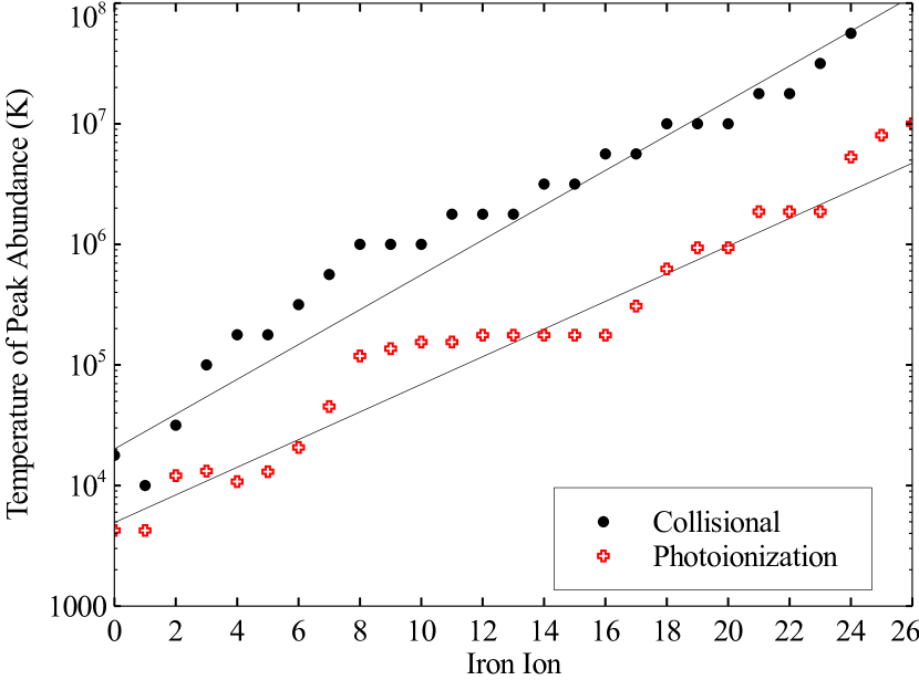
Figure 1: Temperature of peak abundance per iron ion for the collisional and photo ionization cases. The gas is cooler in photoionization equilibrium, which affects the strategy used to compute the cooling rate.

This has two effects on the calculation of the gas cooling. In the collisional ionization case the gas kinetic temperature is not much lower than the ionization energy of the ion. This means that very highly excited levels can be populated by thermal collisions. In the photoionization case the temperature is significantly lower, meaning the the cooling will be dominated by a few lower levels. This affects our strategy in optimizing our selection of the number of levels to include in atomic models.

2.3 Line Cooling

2.3.1 Cloudy Hybrid

We have long included all resonance lines in the TopBase Opacity Project data base (Seaton, 1987), with collision strengths determined from highly approximate g-bar approximations. Adding the Chianti database lines into Cloudy required a decision about how to integrate these databases since some Opacity Project lines may exist within Chianti. The emission spectra for the iron ions we include are shown in Figure 2 and in the online material. These show that the Opacity Project lines tend to occur at wavelengths shorter than the Chianti lines. Chianti only includes lines which have collision strengths computed with sophisticated methods, and only for transitions with the lower level in the ground term (we use the g-bar approximation for subordinate lines). The Opacity Project line data often extend to higher excitation levels. We use the Chianti data for all lines it includes, and supplement these with higher excitation Opacity Project data using the g-bar approximation. We refer to this as the Hybrid scheme.

Figure 2 illustrates how the Opacity Project and Chianti data are blended to give the Hybrid spectrum for one ion stage (the online material shows all ions). Although all calculations are done with Cloudy, we use different parts of the atomic database to compare spectra. The top panel, labeled C10, shows the combination of the internal data and the Opacity Project data that were part of C10, the last major release of Cloudy. The Chianti spectrum (middle panel) shows only lines included in that database, and contains more lines than Opacity Project (C10) at 1000 Å and longer. The C10 spectrum, largely lines in the Opacity Project, has quite a few lines between 100 Å and 1000 Å that are missing from the Chianti spectrum. The Hybrid spectrum (lower panel) is the blending of these two spectra as described previously, containing both the Chianti lines and the Opacity Project lines. The Hybrid configuration will be the default in the next major release of Cloudy.

The addition of the Opacity Project data to Chianti has little effect on the cooling in the photoionization case where kT is relatively lower than the ionization potential. It does increase the cooling in the collisional case where kT approaches the ionization potential and even Rydberg levels can be excited.

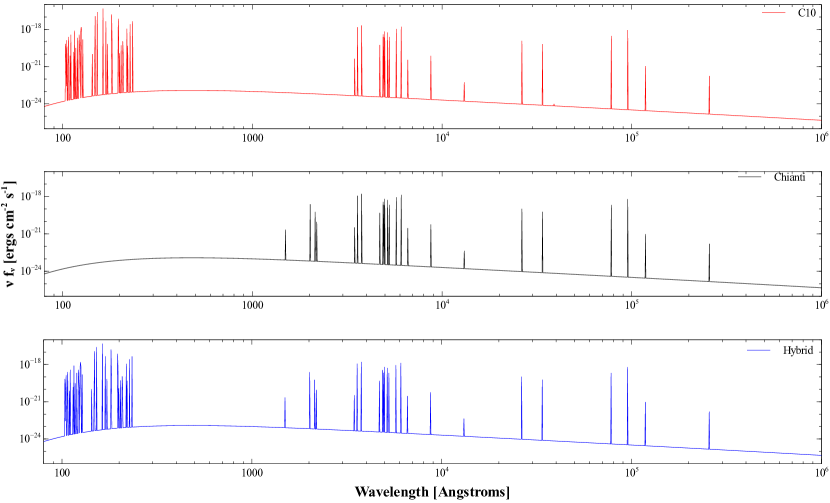
Figure 2: Plots of Fe vii spectra for a collisionally ionized gas under three different Cloudy configurations; Opacity Project with the Cloudy internal database (labelled as C10), Chianti only, and our new default Hybrid configuration (Chianti + Opacity Project). Spectra for other iron ions considered in this paper are shown in the on-line material.

2.3.2 The Kurucz database

Cloudy uses a large model of the Fe ii emission (Verner et al., 1999) and the H-like and He-like ions are treated in the iso-electronic approach described previously. Fe iv through Fe xxiv come from Chianti as described in 2.3.1. The only missing iron ion is Fe²⁺. To fill that void, we added data from the Kurucz database (Kurucz & Bell, 1995) for that ion. This gives energy levels and transition probabilities, but does not contain collision strengths. Collision strengths for the lowest 14 levels of Fe iii are given by Zhang (1996). For the many higher levels we use the g-bar approximation as we did for the Opacity Project. We combine the Zhang (1996) and Kurucz data with the Opacity Project data using the Hybrid scheme described above.

2.4 Iron Cooling

As a test we computed a collisional ionization cooling curve for a pure iron plasma using the three different available databases. The results are shown in Figure 3. The green dashed line is the latest release of Cloudy, known as C10. This uses only our internal database and the Opacity Prtoject and does not contain any data from Chianti or Kurucz. The red dotted line, labeled Chianti+, uses Chianti and Kurucz data, but not the Opacity Project. The Hybrid configuration contains Chianti, the Opacity Project, and our Kurucz additions.

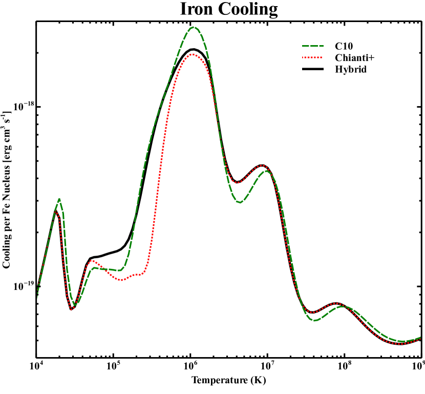
Figure 3: Comparison of the iron cooling per nucleus between the “C10” internal database (the green dashed line), “Chianti+” (Chianti + Kurucz, the red dotted line), and “Hybrid” (Opacity Project + Chianti + Kurucz, the solid black line).

All three configurations have good agreement at the temperature extremes. Between 4$\times 10^{4}$ and 2$\times 10^{5}$  K, the Hybrid configuration has more cooling than the other two. Hybrid has more cooling than C10 in this range because of the addition of the Fe iii Kurucz data as well as Fe iv and Fe v data from Chianti. Hybrid cooling is greater than Chianti+ for this temperature range and up to 5$\times 10^{5}$  K because it has the additional Opacity Project lines.

The C10 cooling exceeds both Hybrid and Chianti+ around 1$\times 10^{6}$  K. This is because C10 used Opacity Project data, with their uncertain g-bar approximation, for many high-excitation iron lines. Chianti uses real calculations of collision strengths and the values for the strongest lines were systematically lower than the g-bar estimates, resulting in less cooling. When a particular transition appears in both data sets, the Opacity Project version is used for C10 and the Chianti version is used for both Hybrid and Chianti+. This is why Hybrid and Chianti+ show equal cooling at many temperatures.

The Hybrid and Chianti+ cooling are equal for temperatures greater than 1$\times 10^{6}$  K. C10 has less cooling in this range because of the additional lines in Chianti. The C10 cooling is different than the other configurations for temperatures above 3$\times 10^{7}$  K due to different ionization distributions, caused in turn by the updates to the recombination coefficients described in Section 2.1.3 that are not present in C10.

In the following sections we will compare our current calculations of the cooling with those presented in previous works. We concentrate on studies which report the cooling for specific elements to remove uncertainties caused by changes in the assumed solar composition. Figure 4 compares the cooling for a pure iron gas for our final Hybrid configuration with the cooling functions of Raymond et al. (1976) and Schure et al. (2009). Raymond et al. (1976) is a standard by which many cooling functions are compared. Our differences from Raymond et al. (1976) are likely the result of their use of g-bar collision strengths. Raymond et al. (1976) used estimation techniques for all collision strengths of Fe i through Fe vii whereas we only use g-bar for Fe iii, the Opacity Project treatment of high-excitation lines, and transitions for which Chianti provides not collision data. The agreement is surprisingly good considering the remarkable changes in the atomic database in the time since their calculation.

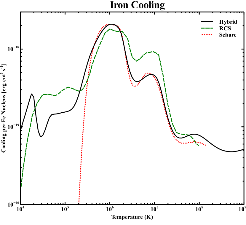
Figure 4: Comparison of the iron cooling per nucleus between the Hybrid configuration of Cloudy, Raymond et al. (1976), and Schure et al. (2009)

Our Hybrid configuration is in good agreement with the Schure et al. (2009) curve at temperatures above 3$\times 10^{5}$  K. At temperatures below 3$\times 10^{5}$  K, the Schure et al. (2009) iron cooling drops off very quickly. Schure et al. (2009) used the package SPEX, which according to the SPEX line list, does not have iron lines at ionizations less than Fe viii. This would explain their lack of iron cooling below 3$\times 10^{5}$  K. Calculations of the total cooling are compared next.

2.5 Total Cooling with our three configurations

The previous sections focused on iron, the element we have expanded to include Chianti data. Here we compute the total cooling of a collisionally-ionized plasma. This depends on all of the elements present, not just iron. For all species other than iron we use our internal database. Figure 5 compares the total cooling for our C10, Chianti+, and Hybrid configurations, using abundances from Raymond et al. (1976). (This composition was chosen to allow later comparisons with their paper.) The Chianti+ and Hybrid configurations give almost identical total cooling, showing that our internal database is in good agreement with Chianti. They are also in reasonable agreement with C10. The C10 total cooling is smaller than the other configurations between 3$\times 10^{6}$ and 2$\times 10^{7}$  K Notice that the updated cooling predicts a region of instability around 6$\times 10^{6}$ K, while the older version predicted that this region have small regions that would have neutral thermal stablility.

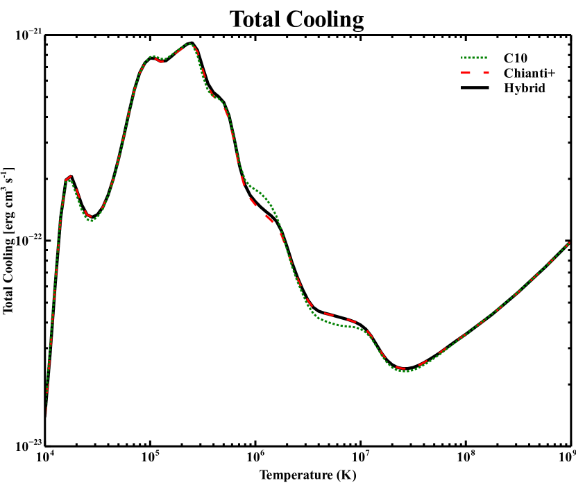
Figure 5: Comparison of the total cooling between the C10, Chianti+, and Hybrid configurations using abundances given in Raymond et al. (1976)

2.5.1 Comparison with Raymond et al. (1976) and Schure et al. (2009)

We compared the iron cooling with Raymond et al. (1976) in section 2.4 and Figure 4, where we found that they produced more cooling between 2$\times 10^{4}$ and 2$\times 10^{5}$  K. Figure 6 compares the total cooling with all elements included. Their total cooling is in surprisingly good agreement with our hybrid scheme considering the major changes in the atomic data that have occurred in the past 35 years.

Figure 6 also shows the total cooling computed by Schure et al. (2009). We compared the iron cooling from Schure et al. (2009) in section 2.4, and found reasonable agreement with our Hybrid configuration for higher temperatures but that their model lacked important coolants below 2$\times 10^{5}$  K. The significantly higher total cooling of Schure et al. (2009) around 10⁵ K cannot be due to iron. Section 2.5.4 explains some possible reasons for this difference.

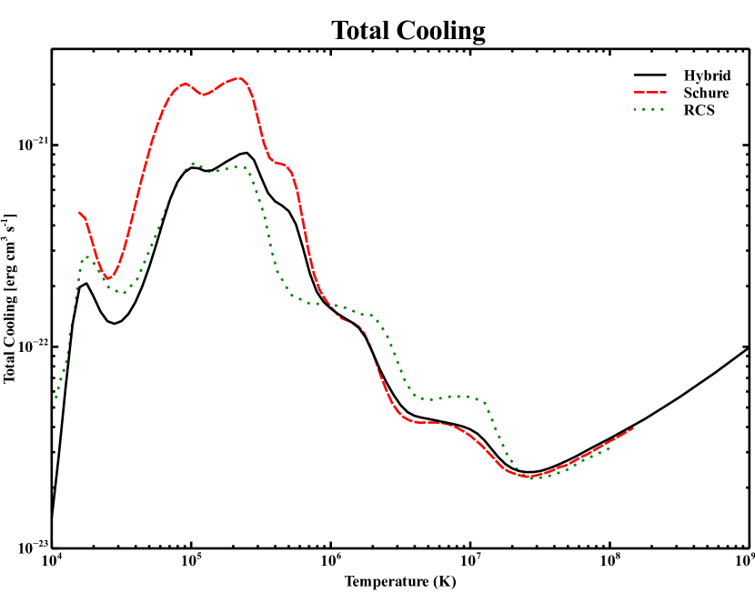
Figure 6: Comparison of the total cooling between the Hybrid configuration of Cloudy, Raymond et al. (1976), and Schure et al. (2009) using abundances of Raymond et al. (1976)

2.5.2 Comparison with Sutherland & Dopita (1993) and Foster et al. (2012)

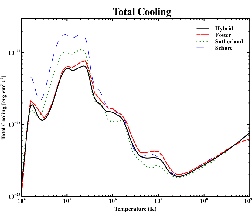
Figure 7: Comparison of the total cooling between our Hybrid configuration, Foster et al. (2012), Sutherland & Dopita (1993), and Schure et al. (2009) using abundances of Anders & Grevesse (1989)

Foster et al. (2012) describes the latest additions to AtomDB, an atomic database that focuses on X-ray astronomy, and which, like Chianti and Cloudy, pays particular attention to the atomic physics. In addition to describing all of the atomic data updated in the latest release of AtomDB, Foster et al. (2012) also provides a total cooling function based on solar abundances of Anders & Grevesse (1989). Sutherland & Dopita (1993) used MAPPINGS II to produce cooling functions between 1$\times 10^{4}$ and 1$\times 10^{8.5}$  K. MAPPINGS II includes calculations for 16 elements with all ion stages.

Figure 7 compares our Hybrid total cooling, Foster et al. (2012), Schure et al. (2009), and Sutherland & Dopita (1993), using the common solar abundances of Anders & Grevesse (1989). The four cooling functions have a similar overall shape. We agree very well with Foster et al. (2012) at all temperatures, specifically around 1$\times 10^{5}$  K where we differ significantly from Schure et al. (2009). However, the cooling at the peak near 1$\times 10^{5}$  K ranges from Hybrid to about a factor of two larger. The Sutherland cooling function lies roughly midway between our Hybrid and Schure et al. (2009). The element or elements causing the difference around 2$\times 10^{5}$  K between Cloudy and Schure et al. (2009) are possibly the same reason for the difference with Sutherland & Dopita (1993). The differences with Schure et al. (2009) are more extreme and we concentrate on that in Section 2.5.4.

2.5.3 Comparison with Colgan et al. (2008)

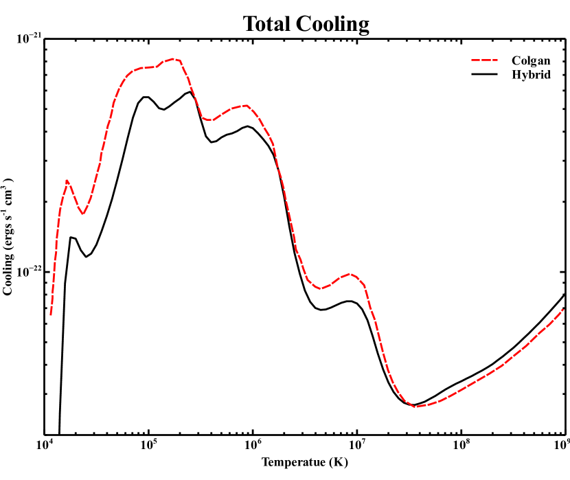
Figure 8: Comparison of the total cooling between Hybrid and Colgan et al. (2008) using the abundances of Colgan et al. (2008)

Colgan et al. (2008) used the Los Alamos plasma kinetics code ATOMIC to calculate radiative losses for a specific set of abundances. They also used several programs that are part of the Los Alamos suite of atomic structure and collision codes to generate the data needed to calculate the losses. Figure 8 compares the Hybrid total cooling function with Colgan et al. (2008). Note that the Colgan et al. (2008) plot has been converted from Watts to ergs. Colgan et al. (2008) find significantly more cooling around 1$\times 10^{5}$  K. Colgan et al. (2008) also compared their total radiative losses with a similar calculation using data from Chianti version 6. Their Chianti 6 results are in reasonable agreement with our Hybrid cooling.

2.5.4 Differences with Schure et al. (2009)

The Schure et al. (2009) cooling curve was produced using the SPEX package using solar abundances from Anders & Grevesse (1989). They provide cooling rates for each element so that their results can be scaled to fit any set of abundances. We used these individual cooling rates to include the Schure et al. (2009) results to Figures 6, 7, and 11. Their calculation shows greater cooling than our Hybrid configuration for $T<10^{6}{\rm\thinspace K}$.

We looked into individual coolants to find the reason for this difference. It is not due to iron since the Schure et al. (2009) iron cooling significantly less than Hybrid around 1$\times 10^{5}$  K  in Figure 4. Cloudy reports that the dominant coolants around 1$\times 10^{5}$  K are carbon and oxygen. In the next section we examine these coolants more closely.

2.6 Carbon and Oxygen Cooling

Figure 9: Comparison of the carbon cooling per nucleus (left) and the oxygen cooling per nucleus (right) for Hybrid, Schure et al. (2009), and Chianti.

The comparison presented above shows that the largest discrepancies occur around 1$\times 10^{5}$  K, regions where the dominant coolants are carbon and oxygen. Figure 9 compares the carbon and oxygen cooling per nucleus for our Hybrid, Schure et al. (2009), and Chianti version 7. Our Hybrid model, which only uses our internal database for these elements, is in good agreement with Chianti. These show that Schure et al. (2009) predict significantly higher cooling below $10^{6}{\rm\thinspace K}$, which accounts for the differences in the total cooling.

The collision strengths are most likely to be the source of the differences in the cooling. We find that the primary carbon cooling transitions at 1$\times 10^{5}$  K are 977 Å of C III and 1548 Å of C IV. For these transitions, Cloudy uses collision strengths from Berrington et al. (1985) and Cochrane & McWhirter (1983) respectively. The C III 977 Å transition is the dominant coolant, contributing 56% of the carbon cooling, while the C IV 1548 Å line contributes about 20%.

The oxygen cooling at 2$\times 10^{5}$  K is dominated by the 630 Å line of O V and a multiplet of 4 O IV lines around 554 Å. Cloudy uses collision strengths from Berrington et al. (1985) for 630 Å. The 554 Å transitions come from the Opacity Project which means that the collision strengths are generated using the g-bar approximation. The dominant line is O V 630 Å with 40% of the oxygen cooling while the O IV 554 Å lines account for 17% of the total.

It is clear from Figure 9 that the carbon and oxygen cooling for Cloudy and Chianti are very similar over the entire temperature range, despite being completely independent implementations of the atomic physics. We compared the sources for the collision data as a check on its reliability. For the 977 and 1548  Å carbon transitions, Chianti uses collision strengths from Berrington et al. (1985) and Griffin et al. (2000) respectively. Cloudy and Chianti use the same source for the 977  Å transition. The Cloudy and Chianti values for the C IV 1548 Å collision strength differ by only 6%.

The results are similar for the oxygen transitions. The Chianti collision strength for 630 Å is 3% less than Cloudy and comes from Berrington (2003; private communication). The 554 Å multiplet uses g-bar collision strengths in Cloudy while Chianti use values from Zhang et al. (1994). The values of the collision strengths differ by only about 5%.

The fact that Schure et al. (2009) find more cooling than Cloudy or Chianti could be explained if they included important cooling lines which are not present in Cloudy or Chianti. C²⁺ and O³⁺ are the dominant stages of ionization at 1$\times 10^{5}$ K and 2$\times 10^{5}$ K respectively. The collisional ionization distribution for hydrogen and helium can be found in Table 1 and for the lightest 30 elements the online version of the table. Schure et al. (2009) used SPEX for its calculations and we were able to compare the SPEX line list to ours and with Chianti. While Chianti has significantly more transitions, there are several transitions in the SPEX line list that are not in Chianti. These transitions are in the tens or few hundreds of Angstroms in wavelength. At temperatures around 1$\times 10^{5}$  K these transitions cannot contribute much cooling due to their small Boltzmann factor. This comparison suggests that the collision rates for the lines mentioned above is the source of the differences.

Unfortunately we cannot compare our collision data with those of Schure et al. (2009), Sutherland & Dopita (1993), and Colgan et al. (2008) because they do not cite sources for, nor give values of, their atomic data. They provide plots for element cooling but not a table of values. The best we can do is to say that three of the four dominant cooling lines around 1$\times 10^{5}$ and 2$\times 10^{5}$  K have two independent sources for collision strengths and that they are in good agreement. This provides us with confidence in our atomic data as well as our cooling functions.

The iron cooling is in good agreement with the cited references above. This is the dominant coolant for higher temperatures. Differences in the carbon and oxygen cooling account for the differences we notice at lower temperatures. The last step is to compare the cooling predicted using Cloudy’s internal atomic data set to Chianti.

2.7 Comparison with the Chianti 7 cooling function

In the hybrid implementation we use Chianti for iron but our internal database for other elements. Here we compare the cooling computed using our database with Chianti. Since we are using Chianti’s iron data in Cloudy Hybrid, we exclude iron in this comparison.

Figure 10 shows this comparison. The Chianti  calculation uses their data for all other species other than the H and He-like iso-sequences where our internal models are used. Since these two calculations use independent implementations of the atomic database, the good agreement between the cooling for all temperatures shows that these databases are in good agreement.

Figure 10: Comparison of the total cooling with the Cloudy internal database and most of Chianti version 7, labelled ”All Chianti+”. Grevesse et al. (2010) abundances are used except that iron is not included. Other than the H and He-like iso-sequences, where our treatment is used for both, these curves use fully independent implementations of the current atomic physics literature. The good agreement suggests that these implementations are complete and in accordance with one another.

2.8 Total cooling in the collisional and photo ionization cases

The goal of this paper is to establish the cooling function used in the Williams et al. (in preparation) calculation of the spectrum of a cooling non-equilibrium plasma. Figure 11 shows our best estimate of the total cooling for the collisional and photoionization cases, using solar abundances from Grevesse et al. (2010). Appendix A provides the Cloudy commands used to create these plots as well as a description of each command. The cooling function for the collisional case is essentially the same as the as the Hybrid cooling functions we have shown in previous plots but with more recent solar abundances. Notice that, with this mix of abundance, the region around 5$\times 10^{6}$ K is thermally stable, whereas it was marginally stable with previous abundance sets. The collisional cooling is given on a per element basis in the Appendix B and a tab-delimited version is available in the online version. Gnat & Ferland (2012) provides element by element cooling using the C10 version of Cloudy. The differences between cooling plots in Gnat & Ferland (2012) and C10 in Figure 3 are due to using different abundances.

The discussion of Figure 1 explains how the photoionization cooling function was calculated. We used the same SED and varied the log of the ionization parameter between -6 and 3, which is the same as Figure 1. The minimum temperature in the plot is 1$\times 10^{4}$  K, to be similar to previous Figures, although the kinetic temperature goes to lower values for low ionization parameter.

Figure 11: The total cooling for the collisional and photo cases of Hybrid Cloudy using solar abundances of Grevesse et al. (2010)

The cooling in the photoionization case is lower than the collisional case at each temperature. The gas kinetic temperature does not play a fundamental a role in photoionization equilibrium, because the ionization is determined by the balance between photoionization and recombination, which have only weak temperature dependences. The cooling rate in the photoionization case is determined by the heating rate, which is set by the SED (AGN3 Chapter 3; Ferland (2003)). The temperature is the result of the interplay between this heating and the gas composition, the so-called “thermostat effect” in photoionization equilibrium (AGN3). The result is the significantly lower kinetic temperature, as shown in both Figures 1 and 11. This distinction will play a major role in our selection of the the default number of levels used to compute the spectra in our new level trimming feature, described below.

2.9 Level trimming

In addition to the experimental iron data, Cloudy can also use the theoretical iron data provided by Chianti. All of the tables and figures in this paper, with the exception of this section, use only experimental Chianti data with no trimming. This section is provided to describe the new capabilities of Cloudy and does not affect any other section of the paper. Some Chianti ions which are of particular interest in the solar case have more than 300 theoretical energy levels and some have as many as 700 levels. The Kurucz database often has thousands of levels. Solving the level populations is quite expensive due to the large number of evaluations of the emission and cooling during the solution of the equations of statistical, thermal, and ionization equilibrium.

We added an option to restrict the maximum number of energy levels that are used for each species. There is a tradeoff between including more levels and lines, which provides a more accurate simulation but with longer run times, versus more compact models, with fewer levels and lines and shorter compute times, but perhaps with some loss of fidelity. This section outlines how we chose the default number of levels, and shows the effects this has on predicted quantities. It is important to note that the level limiting only applies to the newly added Chianti and Kurucz data. All of the data used in C10, including Opacity Project data, are unaffected by this limiting.

Figure 12 shows the total cooling $\Lambda_{ALL}$ (top panel) using all theoretical levels in the Chianti and Kurucz databases, and the cooling with a particular subset of these levels described below. The differences are small. The lower panel shows the relative difference between the full database and our compact model with $n$ levels as $(\Lambda_{ALL}-\Lambda_{n})/\Lambda_{ALL}$. Plots like this one were used to decide on an optimum default limit to the number of levels $n$.

The kinetic temperature in a photoionized gas is lower, for a particular ionization state, than in a collisional gas (Figure 1). As a result, for a given ion, more levels will be energetically accessible in the collisional case compared with the photoionized case. Since we will be adding more of the Chianti species in the future and since Chianti iron species have significantly more energy levels than most other species, we have a default number of levels for iron species and one for all other species. After some experiments we settled on a default limit of 100 levels for the collisional case and 25 levels for the photoionization case for each iron species. For all other Chianti species, which will be added in the future, the default limits are 50 for collisional and 15 for photionization. We find that these limits capture nearly all of the total cooling but requires about five times less compute time than using the full database. This is the approximation shown in the top panel of Figure 12. For the collisional case the limited levels produces cooling within 1% of the total for most temperatures, with the worst agreement of $\sim 5\%$ around ${10^{7}}$ K. This peak error is mostly due to limiting Fe xix to 100 of its 636 levels. The photoionization cooling functions are essentially identical with the smaller number of levels reproducing the total cooling within better than 0.1%.

Since the accuracy required for a specific simulation may depend on particular goals, we provide a simple input option to change the number of levels. All of the plots in this paper are using the full Chianti and Kurucz databases unless otherwise noted.

Figure 12: Total cooling using Chianti theoretical energy levels of Cloudy Hybrid collision and photon dominated cases using all available levels and the default numbers (top) and the associated relative difference (bottom) described in Section 2.9

3 Conclusions

This paper outlines some improvements to the plasma simulation code Cloudy. It will become the reference for future improvements in the atomic and molecular database. The specific results are the following:

• We added much of the experimental iron data provided by Chianti version 7 (Landi et al., 2012). In addition, we added energy levels and transition probabilities from the Kurucz database (Kurucz, 2009) for Fe iii. Those Fe iii data were supplemented by collision strengths using the g-bar approximation. Fe ii is treated with the model described by (Verner et al., 1999) and the H-like and He-like ions are treated with the unified described by Porter & Ferland (2007).

• The Hybrid configuration was added to expand the wavelength coverage of Cloudy by merging the existing Opacity Project data, which we have long included, with the Chianti and Kurucz data. The Opacity Project and Kurucz data do not have corresponding collision rates, and we have used the g-bar approximation to include them.

• We updated Cloudy with the latest recombination coefficients from the Badnell website, including Nikolić et al. (2010) and Abdel-Naby et al. (2012). We updated Cloudy’s collisional ionization rate coefficients to those given in Dere (2007), although these are very similar to the rates of Voronov (1997) which we have used since soon after the publication of that paper. The ionization distributions shown in this paper are based on these updates.

• We added an option to limit the number of energy levels that will be used for a particular simulation in order to reduce run time without sacrificing accuracy. This reproduces the results of the full databases to within much better than 5% but with five times shorted run times. It is easy to change this option with user accessible commands. This limiting was not used to generate any figures or tables in this paper except for Figure 12, which demonstrates the accuracy of the level trimming results.

• Our iron cooling function created with the Hybrid mix of the Opacity Project, Chianti, and Kurucz data agrees surprisingly well with that of Raymond et al. (1976) considering the remarkable changes in the atomic database in the past 35 years. Significant differences exist with Schure et al. (2009) at temperatures below 1$\times 10^{6}$  K. We attribute the difference in iron cooling to missing ions (Fe vii and below) in the SPEX tool.

• The total cooling also agrees with Foster et al. (2012) and when we use the full Chianti database. We find less cooling around 1$\times 10^{5}$  K compared to Schure et al. (2009), Sutherland & Dopita (1993), and Colgan et al. (2008). Detailed comparisons show that differences with Schure et al. (2009) (the calculation where such comparisons are possible) are due to carbon and oxygen cooling. We compared our Hybrid configuration total cooling to the total cooling using the Chianti version 7 data for the majority of the available species and concluded that these two implementations of the atomic data literature are in good agreement. We suspect that the differences in cooling compared with Schure et al. (2009), Sutherland & Dopita (1993), and Colgan et al. (2008) are due to their atomic data, although it is not possible to track down what they used.

• Cloudy is open source and is freely available. Appendix A in the on-line version provides the Cloudy input scripts needed to generate the cooling functions used in this paper.

• We provide detailed ionization and cooling rates for each of the thirty elements included in the calculation in the on-line version.

GJF acknowledges support by NSF (0908877; 1108928; and 1109061), NASA (07-ATFP07-0124, 10-ATP10-0053, and 10-ADAP10-0073), JPL (RSA No 1430426), and STScI (HST-AR-12125.01, GO-12560, and HST-GO-12309). PvH acknowledges support from the Belgian Science Policy Office through the ESA Prodex programme.

Appendix A Input Scripts

We have included the Cloudy input scripts for calculating the cooling in both collisional and photon dominated cases. These are the scripts used to generate Figure 11, which assumes solar abundances. We have also provided a description of each command.

Table 2: Collision dominated cooling of Cloudy Hybrid using solar abundances

coronal 4 vary

atom chianti hybrid ”CloudyChiantiKurucz.ini”

abundances GASS10

atom feii

grid 4 9 0.05

hden 0

stop zone 1

set dr 0

set eden 0

save cooling ”hybrid-coll.col” last no hash

Table 3: Photon dominated cooling of Cloudy Hybrid using solar abundances

table agn

atom chianti hybrid ”CloudyChiantiKurucz.ini”

abundances GASS10

ionization parameter -2 vary

grid -6 3 0.25

hden 0

stop zone 1

save cooling ”hybrid-photo.col” last

coronal 4 vary

Coronal sets up a collisonally ionized gas at 1$\times 10^{4}$  K and vary it based on the grid command.

atom chianti hybrid ”CloudyChiantiKurucz.ini”

This command enables Hybrid mode using all species listed in CloudyChiantiKurucz.ini.

abundances GASS10

This makes Cloudy use the solar abundances from Grevesse et al. (2010).

atom feii

Atom feii enables the Fe ii model developed by Verner et al. (1999).

grid 4 9 0.05

The grid command gives the limits of what is being varied as well as the increment. For Table 2, the temperature is being varied between 1$\times 10^{4}$ and 1$\times 10^{9}$  K in 0.05 dex increments. Table 3 is varying the ionization parameter.

hden 0

Hden sets the log of the total hydrogen density. In this case, it is set to $1{\rm\thinspace cm^{-3}}$.

stop zone 1

Stop zone sets the limit to the number of zone to calculate per iteration.

set dr 0

Set dr sets the log of the zone thickness in cm.

set eden 0

Set eden sets the log of the electron density in ${\rm\thinspace cm^{-3}}$.

table agn

Table AGN sets up the incident radiation field using a continuum from Mathews & Ferland (1987).

ionization parameter -2 vary

The ionization parameter is the dimensionless ratio of hydrogen-ionizing photon to total-hydrogen densities.

save cooling ”hybrid-coll.col” last

This saves the cooling agents for the last zone.

Appendix B Cooling by Element

Table 4: Element specific cooling [erg cm³ s^-1 for the lightest 30 elements which come from revision 6417 of the Cloudy trunk.

Te (K)	Hydrogen	Helium	Lithium	Beryllium	Boron	Carbon	Nitrogen	Oxygen	Fluorine	Neon
1.00E+04	4.32E-24	6.85E-29	6.80E-22	4.93E-21	3.16E-22	6.41E-21	3.11E-21	1.15E-21	2.53E-25	7.63E-28
1.58E+04	1.71E-22	1.26E-25	1.01E-22	2.14E-19	1.58E-20	7.56E-21	1.37E-20	9.04E-21	1.17E-21	1.01E-23
2.51E+04	7.93E-23	2.48E-23	2.67E-23	2.09E-19	1.61E-19	2.93E-20	3.37E-20	2.66E-20	1.06E-20	6.10E-22
3.98E+04	2.82E-23	5.02E-23	1.04E-23	1.20E-20	6.66E-19	1.30E-19	8.05E-20	4.98E-20	1.76E-20	1.34E-21
6.31E+04	1.28E-23	3.58E-22	2.14E-23	1.30E-21	4.77E-19	4.01E-19	1.98E-19	1.25E-19	5.54E-20	2.00E-20
1.00E+05	6.98E-24	6.21E-22	5.59E-22	2.62E-22	3.14E-20	6.49E-19	4.37E-19	2.94E-19	1.83E-19	9.51E-20
1.58E+05	4.48E-24	2.26E-22	1.13E-21	2.03E-22	3.84E-21	7.81E-20	6.72E-19	5.15E-19	3.98E-19	2.73E-19
2.51E+05	3.31E-24	9.86E-23	1.68E-21	1.71E-21	9.10E-22	7.95E-21	9.78E-20	6.87E-19	6.43E-19	4.86E-19
3.98E+05	2.72E-24	5.31E-23	6.76E-22	3.54E-21	1.87E-21	1.73E-21	1.01E-20	9.69E-20	6.78E-19	7.34E-19
6.31E+05	2.55E-24	3.32E-23	3.09E-22	2.16E-21	5.26E-21	2.60E-21	2.57E-21	1.10E-20	7.55E-20	3.88E-19
1.00E+06	2.64E-24	2.42E-23	1.74E-22	9.46E-22	4.32E-21	7.36E-21	4.37E-21	3.69E-21	1.13E-20	3.74E-20
1.58E+06	2.91E-24	2.07E-23	1.11E-22	5.01E-22	1.97E-21	6.16E-21	1.08E-20	7.69E-21	6.14E-21	8.81E-21
2.51E+06	3.35E-24	2.00E-23	8.35E-23	3.07E-22	1.04E-21	2.96E-21	8.04E-21	1.44E-20	1.33E-20	9.50E-21
3.98E+06	3.95E-24	2.10E-23	7.25E-23	2.18E-22	6.27E-22	1.62E-21	4.01E-21	9.23E-21	1.70E-20	1.94E-20
6.31E+06	4.74E-24	2.32E-23	7.02E-23	1.81E-22	4.41E-22	9.99E-22	2.26E-21	4.83E-21	9.70E-21	1.76E-20
1.00E+07	5.75E-24	2.66E-23	7.35E-23	1.69E-22	3.60E-22	7.24E-22	1.45E-21	2.84E-21	5.38E-21	9.76E-21
1.58E+07	7.08E-24	3.15E-23	8.16E-23	1.73E-22	3.34E-22	6.08E-22	1.09E-21	1.93E-21	3.35E-21	5.68E-21
2.51E+07	8.76E-24	3.79E-23	9.41E-23	1.89E-22	3.40E-22	5.76E-22	9.49E-22	1.54E-21	2.44E-21	3.82E-21
3.98E+07	1.09E-23	4.61E-23	1.11E-22	2.15E-22	3.71E-22	5.96E-22	9.23E-22	1.39E-21	2.07E-21	3.02E-21
6.31E+07	1.35E-23	5.65E-23	1.34E-22	2.52E-22	4.22E-22	6.55E-22	9.73E-22	1.40E-21	1.97E-21	2.73E-21
1.00E+08	1.69E-23	6.97E-23	1.63E-22	3.02E-22	4.94E-22	7.50E-22	1.08E-21	1.51E-21	2.06E-21	2.74E-21
1.58E+08	2.12E-23	8.67E-23	2.01E-22	3.68E-22	5.94E-22	8.88E-22	1.26E-21	1.72E-21	2.28E-21	2.97E-21
2.51E+08	2.67E-23	1.08E-22	2.48E-22	4.52E-22	7.23E-22	1.07E-21	1.50E-21	2.02E-21	2.64E-21	3.38E-21
3.98E+08	3.37E-23	1.35E-22	3.08E-22	5.58E-22	8.88E-22	1.30E-21	1.81E-21	2.42E-21	3.13E-21	3.96E-21
6.31E+08	4.30E-23	1.69E-22	3.84E-22	6.92E-22	1.10E-21	1.60E-21	2.21E-21	2.94E-21	3.78E-21	4.74E-21
1.00E+09	5.56E-23	2.11E-22	4.79E-22	8.60E-22	1.36E-21	1.98E-21	2.72E-21	3.59E-21	4.60E-21	5.76E-21

Table 5: Element specific cooling [erg cm³ s^-1 for the lightest 30 elements - continued

Te (K)	Sodium	Magnesium	Aluminium	Silicon	Phosphorus	Sulphur	Chlorine	Argon	Potassium	Calcium
1.00E+04	9.48E-23	1.85E-20	1.08E-20	1.36E-20	5.56E-21	2.03E-20	4.34E-21	8.91E-24	2.96E-23	3.31E-19
1.58E+04	1.64E-23	1.29E-19	7.46E-20	3.38E-20	2.44E-20	1.13E-19	5.81E-20	5.34E-21	8.09E-24	2.25E-19
2.51E+04	4.98E-24	1.80E-20	2.81E-19	1.47E-19	7.30E-20	1.61E-19	8.99E-20	1.31E-20	5.99E-23	1.14E-20
3.98E+04	3.62E-23	1.34E-21	6.30E-19	4.74E-19	2.13E-19	2.42E-19	1.68E-19	6.44E-20	1.52E-20	2.97E-21
6.31E+04	1.98E-21	2.43E-22	3.72E-20	9.23E-19	6.48E-19	7.50E-19	1.13E-19	2.45E-19	1.33E-19	4.78E-20
1.00E+05	1.81E-20	2.22E-21	4.10E-21	8.18E-19	1.46E-18	1.55E-18	1.38E-19	8.28E-19	6.73E-19	2.57E-19
1.58E+05	9.69E-20	3.26E-20	4.63E-21	2.02E-20	2.44E-19	1.61E-18	7.12E-19	1.75E-18	1.16E-18	9.54E-19
2.51E+05	2.85E-19	1.61E-19	5.27E-20	1.60E-20	2.46E-20	7.22E-20	1.39E-18	2.53E-18	1.04E-18	1.90E-18
3.98E+05	4.85E-19	4.14E-19	1.94E-19	9.84E-20	3.35E-20	1.09E-20	1.38E-19	8.43E-19	1.22E-18	2.53E-18
6.31E+05	6.33E-19	6.75E-19	3.75E-19	2.99E-19	1.26E-19	6.88E-20	6.20E-20	1.11E-19	3.30E-19	1.29E-18
1.00E+06	1.82E-19	5.38E-19	5.33E-19	5.45E-19	2.54E-19	2.38E-19	9.17E-20	1.12E-19	1.10E-19	1.93E-19
1.58E+06	2.41E-20	6.16E-20	2.91E-19	4.73E-19	3.28E-19	4.23E-19	5.08E-20	2.47E-19	8.84E-20	1.67E-19
2.51E+06	1.02E-20	1.43E-20	3.79E-20	7.83E-20	2.11E-19	4.10E-19	2.79E-20	4.05E-19	4.86E-20	3.00E-19
3.98E+06	1.64E-20	1.33E-20	1.52E-20	2.02E-20	3.71E-20	5.69E-20	1.17E-20	2.83E-19	3.38E-20	4.21E-19
6.31E+06	2.40E-20	2.47E-20	2.19E-20	1.93E-20	2.03E-20	1.36E-20	7.30E-21	3.89E-20	1.30E-20	1.92E-19
1.00E+07	1.65E-20	2.51E-20	3.20E-20	3.23E-20	2.98E-20	2.08E-20	1.51E-20	1.87E-20	1.18E-20	3.47E-20
1.58E+07	9.51E-21	1.53E-20	2.35E-20	3.22E-20	3.86E-20	3.76E-20	3.37E-20	3.11E-20	2.45E-20	2.67E-20
2.51E+07	6.01E-21	9.26E-21	1.40E-20	2.06E-20	2.88E-20	3.65E-20	4.28E-20	4.63E-20	4.44E-20	4.30E-20
3.98E+07	4.43E-21	6.42E-21	9.21E-21	1.31E-20	1.83E-20	2.44E-20	3.21E-20	4.05E-20	4.74E-20	5.28E-20
6.31E+07	3.78E-21	5.17E-21	7.03E-21	9.51E-21	1.28E-20	1.65E-20	2.16E-20	2.78E-20	3.49E-20	4.27E-20
1.00E+08	3.63E-21	4.75E-21	6.16E-21	7.97E-21	1.02E-20	1.28E-20	1.62E-20	2.03E-20	2.53E-20	3.11E-20
1.58E+08	3.81E-21	4.83E-21	6.06E-21	7.56E-21	9.38E-21	1.14E-20	1.39E-20	1.70E-20	2.05E-20	2.47E-20
2.51E+08	4.25E-21	5.27E-21	6.47E-21	7.87E-21	9.51E-21	1.13E-20	1.35E-20	1.60E-20	1.89E-20	2.22E-20
3.98E+08	4.93E-21	6.03E-21	7.29E-21	8.72E-21	1.04E-20	1.22E-20	1.42E-20	1.66E-20	1.92E-20	2.21E-20
6.31E+08	5.85E-21	7.10E-21	8.50E-21	1.01E-20	1.18E-20	1.38E-20	1.59E-20	1.83E-20	2.09E-20	2.38E-20
1.00E+09	7.06E-21	8.52E-21	1.01E-20	1.19E-20	1.39E-20	1.61E-20	1.85E-20	2.11E-20	2.39E-20	2.70E-20

Table 6: Element specific cooling [erg cm³ s^-1 for the lightest 30 elements - continued

Te (K)	Scandium	Titanium	Vanadium	Chromium	Manganese	Iron	Cobalt	Nickel	Copper	Zinc
1.00E+04	3.77E-19	1.42E-19	1.35E-20	5.28E-21	5.37E-20	8.84E-20	2.74E-21	5.26E-21	1.07E-21	5.83E-21
1.58E+04	5.24E-19	4.91E-19	7.65E-20	5.44E-20	3.50E-19	2.16E-19	3.49E-20	8.16E-21	2.37E-21	1.25E-19
2.51E+04	9.27E-20	1.39E-19	3.57E-20	1.17E-19	1.85E-19	9.70E-20	1.97E-20	2.77E-20	1.26E-20	2.53E-19
3.98E+04	8.02E-21	5.90E-20	7.25E-20	1.06E-19	1.31E-20	1.12E-19	2.76E-20	4.72E-21	2.58E-21	3.47E-20
6.31E+04	1.23E-20	1.68E-20	4.86E-20	1.04E-19	1.05E-21	1.46E-19	1.42E-20	6.48E-22	5.39E-22	5.48E-21
1.00E+05	1.58E-19	6.73E-20	3.53E-20	7.22E-20	1.53E-21	1.55E-19	2.07E-21	1.03E-21	9.20E-22	3.57E-21
1.58E+05	5.39E-19	4.37E-19	2.69E-19	1.49E-19	1.38E-20	1.83E-19	2.55E-21	2.28E-21	2.23E-21	2.38E-21
2.51E+05	3.31E-19	8.62E-19	9.33E-19	6.89E-19	3.50E-19	4.04E-19	1.95E-20	6.84E-21	6.35E-21	5.57E-21
3.98E+05	2.50E-19	3.72E-19	1.07E-18	1.42E-18	1.27E-18	9.57E-19	3.45E-19	1.74E-20	1.52E-20	1.38E-20
6.31E+05	1.06E-18	4.09E-19	9.72E-19	1.30E-18	1.76E-18	1.61E-18	1.35E-18	1.09E-19	3.49E-20	3.39E-20
1.00E+06	4.35E-19	9.17E-19	1.20E-18	1.38E-18	8.44E-19	2.08E-18	2.08E-18	9.56E-19	7.07E-20	7.07E-20
1.58E+06	1.73E-19	2.49E-19	4.11E-19	7.39E-19	7.28E-19	1.86E-18	1.59E-18	1.52E-18	9.60E-20	9.92E-20
2.51E+06	1.85E-19	1.88E-19	2.10E-19	2.53E-19	3.79E-19	6.53E-19	8.78E-19	1.08E-18	1.38E-19	1.36E-19
3.98E+06	2.15E-19	2.04E-19	2.13E-19	2.19E-19	2.44E-19	3.80E-19	3.32E-19	4.16E-19	6.05E-20	1.14E-19
6.31E+06	2.19E-19	1.98E-19	2.02E-19	2.01E-19	2.19E-19	4.41E-19	2.83E-19	3.02E-19	4.85E-20	5.07E-20
1.00E+07	7.69E-20	1.05E-19	1.47E-19	1.56E-19	1.60E-19	4.59E-19	2.17E-19	2.51E-19	7.00E-20	6.76E-20
1.58E+07	4.14E-20	4.89E-20	6.24E-20	7.58E-20	9.50E-20	2.19E-19	1.45E-19	1.62E-19	7.27E-20	8.13E-20
2.51E+07	4.67E-20	4.66E-20	4.80E-20	5.11E-20	5.67E-20	8.91E-20	6.99E-20	8.97E-20	3.86E-20	4.75E-20
3.98E+07	5.72E-20	5.86E-20	5.87E-20	5.87E-20	5.90E-20	7.16E-20	5.84E-20	6.39E-20	4.08E-20	4.25E-20
6.31E+07	5.10E-20	5.82E-20	6.40E-20	6.82E-20	7.08E-20	7.88E-20	7.19E-20	7.32E-20	6.30E-20	6.49E-20
1.00E+08	3.74E-20	4.54E-20	5.36E-20	6.12E-20	6.85E-20	7.77E-20	8.01E-20	8.47E-20	8.45E-20	9.11E-20
1.58E+08	2.88E-20	3.53E-20	4.21E-20	4.85E-20	5.61E-20	6.49E-20	7.21E-20	8.01E-20	8.68E-20	9.77E-20
2.51E+08	2.51E-20	3.03E-20	3.56E-20	4.05E-20	4.67E-20	5.38E-20	6.09E-20	6.88E-20	7.68E-20	8.73E-20
3.98E+08	2.48E-20	2.91E-20	3.34E-20	3.76E-20	4.27E-20	4.85E-20	5.46E-20	6.14E-20	6.85E-20	7.70E-20
6.31E+08	2.65E-20	3.05E-20	3.44E-20	3.84E-20	4.30E-20	4.81E-20	5.35E-20	5.96E-20	6.59E-20	7.30E-20
1.00E+09	3.00E-20	3.39E-20	3.78E-20	4.19E-20	4.65E-20	5.14E-20	5.67E-20	6.24E-20	6.84E-20	7.50E-20

References

- Abdel-Naby et al. (2012) Abdel-Naby S. A., Nikolić D., Gorczyca T. W., Korista K. T., Badnell N. R., 2012, A&A, 537, A40
- Ali et al. (1991) Ali B., Blum R. D., Bumgardner T. E., Cranmer S. R., Ferland G. J., Haefner R. I., Tiede G. P., 1991, PASP, 103, 1182
- Anders & Grevesse (1989) Anders E., Grevesse N., 1989, Geochim. Cosmochim. Acta, 53, 197
- Badnell (2006) Badnell N. R., 2006, ApJS, 167, 334
- Badnell et al. (2003) Badnell N. R., O’Mullane M. G., Summers H. P., Altun Z., Bautista M. A., Colgan J., Gorczyca T. W., Mitnik D. M., Pindzola M. S., Zatsarinny O., 2003, A&A, 406, 1151
- Berrington et al. (1985) Berrington K. A., Burke P. G., Dufton P. L., Kingston A. E., 1985, Atomic Data and Nuclear Data Tables, 33, 195
- Cochrane & McWhirter (1983) Cochrane D. M., McWhirter R. W. P., 1983, Phys. Scr, 28, 25
- Colgan et al. (2008) Colgan J., Abdallah Jr. J., Sherrill M. E., Foster M., Fontes C. J., Feldman U., 2008, ApJ, 689, 585
- Dere (2007) Dere K. P., 2007, A&A, 466, 771
- Dere et al. (1997) Dere K. P., Landi E., Mason H. E., Monsignori Fossi B. C., Young P. R., 1997, A&AS, 125, 149
- Ferland (2003) Ferland G. J., 2003, ARA&A, 41, 517
- Ferland et al. (1998) Ferland G. J., Korista K. T., Verner D. A., Ferguson J. W., Kingdon J. B., Verner E. M., 1998, PASP, 110, 761
- Foster et al. (2012) Foster A. R., Ji L., Smith R. K., Brickhouse N. S., 2012, ArXiv e-prints
- Gaetz & Salpeter (1983) Gaetz T. J., Salpeter E. E., 1983, ApJS, 52, 155
- Gnat & Ferland (2012) Gnat O., Ferland G. J., 2012, ApJS, 199, 20
- Grevesse et al. (2010) Grevesse N., Asplund M., Sauval A. J., Scott P., 2010, Ap&SS, 328, 179
- Griffin et al. (2000) Griffin D. C., Badnell N. R., Pindzola M. S., 2000, Journal of Physics B Atomic Molecular Physics, 33, 1013
- Gu (2002) Gu M., 2002, APS Meeting Abstracts, pp 17075–+
- Kato (1976) Kato T., 1976, ApJS, 30, 397
- Kurucz (2009) Kurucz R. L., 2009, in I. Hubeny, J. M. Stone, K. MacGregor, & K. Werner ed., American Institute of Physics Conference Series Vol. 1171 of American Institute of Physics Conference Series, Including All the Lines. pp 43–51
- Kurucz & Bell (1995) Kurucz R. L., Bell B., 1995, Atomic line list
- Landi et al. (2012) Landi E., Del Zanna G., Young P. R., Dere K. P., Mason H. E., 2012, ApJ, 744, 99
- Luridiana et al. (2009) Luridiana V., Simón-Díaz S., Cerviño M., Delgado R. M. G., Porter R. L., Ferland G. J., 2009, ApJ, 691, 1712
- Mathews & Ferland (1987) Mathews W. G., Ferland G. J., 1987, ApJ, 323, 456
- Mewe (1972) Mewe R., 1972, A&A, 20, 215
- Mewe et al. (1985) Mewe R., Gronenschild E. H. B. M., van den Oord G. H. J., 1985, A&AS, 62, 197
- Nikolić et al. (2010) Nikolić D., Gorczyca T. W., Korista K. T., Badnell N. R., 2010, A&A, 516, A97+
- Osterbrock & Ferland (2006) Osterbrock D. E., Ferland G. J., 2006, Astrophysics of gaseous nebulae and active galactic nuclei, 2nd. ed.. Sausalito, CA: University Science Books
- Porter et al. (2005) Porter R. L., Bauman R. P., Ferland G. J., MacAdam K. B., 2005, ApJ, 622, L73
- Porter & Ferland (2007) Porter R. L., Ferland G. J., 2007, ApJ, 664, 586
- Raymond et al. (1976) Raymond J. C., Cox D. P., Smith B. W., 1976, ApJ, 204, 290
- Schure et al. (2009) Schure K. M., Kosenko D., Kaastra J. S., Keppens R., Vink J., 2009, A&A, 508, 751
- Seaton (1987) Seaton M., 1987, Journal of Physics B Atomic Molecular Physics, 20, 6363
- Shaw et al. (2005) Shaw G., Ferland G. J., Abel N. P., Stancil P. C., van Hoof P. A. M., 2005, ApJ, 624, 794
- Sutherland & Dopita (1993) Sutherland R. S., Dopita M. A., 1993, ApJS, 88, 253
- Verner et al. (1996) Verner D. A., Verner E. M., Ferland G. J., 1996, Atomic Data and Nuclear Data Tables, 64, 1
- Verner et al. (1999) Verner E. M., Verner D. A., Korista K. T., Ferguson J. W., Hamann F., Ferland G. J., 1999, ApJS, 120, 101
- Voronov (1997) Voronov G. S., 1997, Atomic Data and Nuclear Data Tables, 65, 1
- Zhang (1996) Zhang H., 1996, A&AS, 119, 523
- Zhang et al. (1994) Zhang H. L., Graziani M., Pradhan A. K., 1994, A&A, 283, 319