Multilevel Monte Carlo methods
for applications in finance
Abstract
Since Giles introduced the multilevel Monte Carlo path simulation method [18], there has been rapid development of the technique for a variety of applications in computational finance. This paper surveys the progress so far, highlights the key features in achieving a high rate of multilevel variance convergence, and suggests directions for future research.
1 Introduction
In 2001, Heinrich [28], developed a multilevel Monte Carlo method for parametric integration, in which one is interested in estimating the value of where is a finite-dimensional random variable and is a parameter. In the simplest case in which is a real variable in the range , having estimated the value of and , one can use as a control variate when estimating the value of , since the variance of will usually be less than the variance of . This approach can then be applied recursively for other intermediate values of , yielding large savings if is sufficiently smooth with respect to .
Giles’ multilevel Monte Carlo path simulation [18] is both similar and different. There is no parametric integration, and the random variable is infinite-dimensional, corresponding to a Brownian path in the original paper. However, the control variate viewpoint is very similar. A coarse path simulations is used as a control variate for a more refined fine path simulation, but since the exact expectation for the coarse path is not known, this is in turn estimated recursively using even coarser path simulation as control variates. The coarsest path in the multilevel hierarchy may have only one timestep for the entire interval of interest.
A similar two-level strategy was developed slightly earlier by Kebaier [31], and a similar multi-level approach was under development at the same time by Speight [42, 43].
In this review article, we start by introducing the central ideas in multilevel Monte Carlo simulation, and the key theorem from [18] which gives the greatly improved computational cost if a number of conditions are satisfied. The challenge then is to construct numerical methods which satisfy these conditions, and we consider this for a range of computational finance applications.
2 Multilevel Monte Carlo
2.1 Monte Carlo
Monte Carlo simulation has become an essential tool in the pricing of derivatives security and in risk management. In the abstract setting, our goal is to numerically approximate the expected value , where is a functional of a random variable . In most financial applications we are not able to sample directly and hence, in order to perform Monte Carlo simulations we approximate with such that , when . Using to compute approximation samples produces the standard Monte Carlo estimate
where is the numerical approximation to on the th sample path and is the number of independent simulations of . By standard Monte Carlo results , when and . In practice we perform Monte Carlo simulation with given and finite producing an error to the approximation of . Here we are interested in the mean square error that is
Our goal in the design of the Monte Carlo algorithm is to estimate with accuracy root-mean-square error (), as efficiently as possible. That is to minimize the computational complexity required to achieve the desired mean square error. For standard Monte Carlo simulations the mean square error can be expressed as
The Monte Carlo variance is proportional to
For both Euler-Maruyama and Milstein approximation , typically. Hence the mean square error for standard Monte Carlo is given by
To ensure the root-mean-square error is proportional to , we must have and therefore and , which means and . The computational cost of standard Monte Carlo is proportional to the number of paths multiplied by the cost of generating a path, that is the number of timesteps in each sample path. Therefore, the cost is . In the next section we will show that using MLMC we can reduce the complexity of achieving root mean square error to .
2.2 Multilevel Monte Carlo Theorem
In its most general form, multilevel Monte Carlo (MLMC) simulation uses a number of levels of resolution, , with being the coarsest, and being the finest. In the context of a SDE simulation, level may have just one timestep for the whole time interval , whereas level might have uniform timesteps .
If denotes the payoff (or other output functional of interest), and denotes its approximation on level , then the expected value on the finest level is equal to the expected value on the coarsest level plus a sum of corrections which give the difference in expectation between simulations on successive levels,
| (1) |
The idea behind MLMC is to independently estimate each of the expectations on the right-hand side of (1) in a way which minimises the overall variance for a given computational cost. Let be an estimator for using samples, and let , , be an estimator for using samples. The simplest estimator is a mean of independent samples, which for is
| (2) |
The key point here is that should come from two discrete approximations for the same underlying stochastic sample (see [39]), so that on finer levels of resolution the difference is small (due to strong convergence) and so its variance is also small. Hence very few samples will be required on finer levels to accurately estimate the expected value.
The combined MLMC estimator is
We can observe that
and
Although we are using different levels with different discretization errors to estimate , the final accuracy depends on the accuracy of the finest level .
Here we recall the Theorem from [18] (which is a slight generalisation of the original theorem in [18]) which gives the complexity of MLMC estimation.
Theorem 2.1.
Let denote a functional of the solution of a stochastic differential equation, and let denote the corresponding level numerical approximation. If there exist independent estimators based on Monte Carlo samples, and positive constants such that and
-
i)
-
ii)
-
iii)
-
iv)
where is the computational complexity of
then there exists a positive constant such that for any there are values and for which the multilevel estimator
has a mean-square-error with bound
with a computational complexity with bound
2.3 Improved MLMC
In the previous section we showed that the key step in MLMC analysis is the estimation of variance . As it will become more clear in the next section, this is related to the strong convergence results on approximations of SDEs, which differentiates MLMC from standard MC, where we only require a weak error bound for approximations of SDEs.
We will demonstrate that in fact the classical strong convergence may not be necessary for a good MLMC variance. In (2) we have used the same estimator for the payoff on every level , and therefore (1) is a trivial identity due to the telescoping summation. However, in [17] Giles demonstrated that it can be better to use different estimators for the finer and coarser of the two levels being considered, when level is the finer level, and when level is the coarser level. In this case, we require that
| (3) |
so that
The MLMC Theorem is still applicable to this modified estimator. The advantage is that it gives the flexibility to construct approximations for which is much smaller than the original , giving a larger value for , the rate of variance convergence in condition iii) in the theorem. In the next sections we demonstrate how suitable choices of and can dramatically increase the convergence of the variance of the MLMC estimator.
The good choice of estimators, as we shall see, often follows from analysis of the problem under consideration from the distributional point of view. We will demonstrate that methods that had been used previously to improve the weak order of convergence can also improve the order of convergence of the MLMC variance.
2.4 SDEs
First, we consider a general class of -dimensional SDEs driven by Brownian motion. These are the primary object of studies in mathematical finance. In subsequent sections we demonstrate extensions of MLMC beyond the Brownian setting.
Let be a complete probability space with a filtration satisfying the usual conditions, and let be a -dimensional Brownian motion defined on the probability space. We consider the numerical approximation of SDEs of the form
| (4) |
where for each , , , and for simplicity we assume a fixed initial value . The most prominent example of SDEs in finance is a geometric Brownian motion
where . Although, we can solve this equation explicitly it is still worthwhile to approximate its solution numerically in order to judge the performance of the numerical procedure we wish to apply to more complex problems. Another interesting example is the famous Heston stochastic volatility model
| (5) |
where . In this case we do not know the explicit form of the solution and therefore numerical integration is essential in order to price certain financial derivatives using the Monte Carlo method. At this point we would like to point out that the Heston model (5) does not satisfy standard conditions required for numerical approximations to converge. Nevertheless, in this paper we always assume that coefficients of SDEs (4) are sufficiently smooth. We refer to [32, 35, 44] for an overview of the methods that can be applied when the global Lipschitz condition does not hold. We also refer the reader to [33] for an application of MLMC to the SDEs with additive fractional noise.
2.5 Euler and Milstein discretisations
The simplest approximation of SDEs (4) is an Euler-Maruyama (EM) scheme. Given any step size , we define the partition of the time interval , . The EM approximation has the form [34]
| (6) |
where and . Equation (6) is written in a vector form and its component reads as
In the classical Monte Carlo setting we are mainly interested in the weak approximation of SDEs (4). Given a smooth payoff we say that converges to in a weak sense with order if
Rate is required in condition of Theorem 2.1. However, for MLMC condition of Theorem 2.1 is crucial.We have
and
For Lipschitz continuous payoffs, , we then have
It is clear now, that in order to estimate the variance of the MLMC we need to examine strong convergence property. The classical strong convergence on the finite time interval is defined as
For the EM scheme . In order to deal with path dependent options we often require measure the error in the supremum norm:
Even in the case of globally Lipschitz continuous payoff , the EM does not achieve which is optimal in Theorem (2.1). In order to improve the convergence of the MLMC variance the Milstein approximation is considered, with component of the form [34]
| (7) |
where is the correlation matrix for the driving Brownian paths, and is the Lévy area defined as
The rate of strong convergence for the Milstein scheme is double the value we have for the EM scheme and therefore the MLMC variance for Lipschitz payoffs converges twice as fast. However, this gain does not come without a price. There is no efficient method to simulate Lévy areas, apart from dimension 2 [14, 41, 45]. In some applications, the diffusion coefficient satisfies a commutativity property which gives
In that case, because the Lévy areas are anti-symmetric (i.e. ), it follows that and therefore the terms involving the Lévy areas cancel and so it is not necessary to simulate them. However, this only happens in special cases. Clark & Cameron [9] proved for a particular SDE that it is impossible to achieve a better order of strong convergence than the Euler-Maruyama discretisation when using just the discrete increments of the underlying Brownian motion. The analysis was extended by Müller-Gronbach [38] to general SDEs. As a consequence if we use the standard MLMC method with the Milstein scheme without simulating the Lévy areas the complexity will remain the same as for Euler-Maruyama. Nevertheless, Giles and Szpruch showed in [22] that by constructing a suitable antithetic estimator one can neglect the Lévy areas and still obtain a multilevel correction estimator with a variance which decays at the same rate as the scalar Milstein estimator.
2.6 MLMC algorithm
Here we explain how to implement the Monte Carlo algorithm. Let us recall that the MLMC estimator is given by
We aim to minimize the computational cost necessary to achieve desirable accuracy . As for standard Monte Carlo we have
The variance is given by
where . To minimize the variance of for fixed computational cost , we can treat as continuous variable and use the Lagrange function to find the minimum of
First order conditions shows that , therefore
Since we want we can show that
thus the optimal number of samples for level is
| (8) |
Assuming weak convergence, the bias of the overall method is equal . If we want the bias to be proportional to we set
From here we can calculate the overall complexity. We can now outline the algorithm
-
1.
Begin with L=0;
-
2.
Calculate the initial estimate of using 100 samples.
-
3.
Determine optimal using (8).
-
4.
Generate additional samples as needed for new .
-
5.
if set and go to 2.
Most numerical tests suggests that is not optimal and we can substantially improve MLMC by determining optimal by looking at bias. For more details see [18].
3 Pricing with MLMC
A key application of MLMC is to compute the expected payoff of financial options. We have demonstrated that for globally Lipschitz European payoffs, convergence of the MLMC variance is determined by the strong rate of convergence of the corresponding numerical scheme. However, in many financial applications payoffs are not smooth or are path-dependent. The aim of this section is to overview results on mean square convergence rates for Euler–Maruyama and Milstein approximations with more complex payoffs. In the case of EM, the majority of payoffs encountered in practice have been analyzed in Giles et al. [20]. Extension of this analysis to the Milstein scheme is far from obvious. This is due to the fact that Milstein scheme gives an improved rate of convergence on the grid points, but this is insufficient for path dependent options. In many applications the behaviour of the numerical approximation between grid points is crucial. The analysis of Milstein scheme for complex payoffs was carried out in [11]. To understand this problem better, we recall a few facts from the theory of strong convergence of numerical approximations. We can define a piecewise linear interpolation of a numerical approximation within the time interval as
| (9) |
where . Müller-Gronbach [37] has show that for the Milstein scheme (9) we have
| (10) |
that is the same as for the EM scheme. In order to maintain the strong order of convergence we use Brownian Bridge interpolation rather than basic piecewise linear interpolation:
| (11) |
for . For the Milstein scheme interpolated with Brownian bridges we have [37]
Clearly is not implementable, since in order to construct it, the knowledge of the whole trajectory is required. However, we will demonstrate that combining with conditional Monte Carlo techniques can dramatically improve the convergence of the variance of the MLMC estimator. This is due to the fact that for suitable MLMC estimators only distributional knowledge of certain functionals of will be required.
3.1 Euler-Maruyama scheme
In this section we demonstrate how to approximate the most common payoffs using the EM scheme (6).
The Asian option we consider has the payoff
Using the piecewise linear interpolation (9) one can obtain the following approximation
Lookback options have payoffs of the form
A numerical approximation to this payoff is
For both of these payoffs it can be proved that [20].
We now consider a digital option, which pays one unit if the asset at the final time exceeds the fixed strike price , and pays zero otherwise. Thus, the discontinuous payoff function has the form
with the corresponding EM value
Assuming boundedness of the density of the solution to (4) in the neighborhood of the strike , it has been proved in [20] that , for any . This result has been tightened by Avikainen [3] who proved that .
An up-and-out call gives a European payoff if the asset never exceeds the barrier, , otherwise it pays zero. So, for the exact solution we have
and for the EM approximation
A down-and-in call knocks in when the minimum asset price dips below the barrier , so that
and, accordingly,
For both of these barrier options we have , for any , assuming that and have bounded density in the neighborhood of [20].
| Euler | ||
|---|---|---|
| option | numerical | analysis |
| Lipschitz | ||
| Asian | ||
| lookback | ||
| barrier | ||
| digital | ||
3.2 Milstein scheme
In the scalar case of SDEs (4) (that is with ) the Milstein scheme has the form
| (12) |
where . The analysis of Lipschitz European payoffs and Asian options with Milstein scheme is analogous to EM scheme and it has been proved in [11] that in both these cases .
3.2.1 Lookback options
For clarity of the exposition
we will express the fine time-step approximation in terms of the coarse time-step, that is
. The partition for the coarse approximation is given by . Therefore,
corresponds to for .
For pricing lookback options with the EM scheme, as an approximation of the minimum of the process we have simply taken
. This approximation could be improved by taking
Here is a constant which corrects the leading order error due to the discrete sampling of the path, and thereby restores weak convergence [6]. However, using this approximation, the difference between the computed minimum values and the fine and coarse paths is , and hence the variance is , corresponding to . In the previous section, this was acceptable because was the best that could be achieved in general with the Euler path discretisation which was used, but we now aim to achieve an improved convergence rate using the Milstein scheme.
In order to improve the convergence, the Brownian Bridge interpolant defined in (11) is used. We have
where minimum of the fine approximation over the first half of the coarse time-step is given by [24]
| (13) |
and minimum of the fine approximation over the second half of the coarse time-step is given by
| (14) |
where are uniform random variables on the unit interval. For the coarse path, in order to improve the MLMC variance a slightly different estimator is used, see (3). Using the same Brownian increments as we used on the fine path (to guarantee that we stay on the same path), equation (11) is used to define . Given this interpolated value, the minimum value over the interval can then be taken to be the smaller of the minima for the two intervals and ,
Note that is used for both time steps. It is because we used the Brownian Bridge with diffusion term to derive both minima. If we changed to in , this would mean that different Brownian Bridges were used on the first and second half of the coarse time-step and as a consequence condition (3) would be violated. Note also the re-use of the same uniform random numbers and used to compute the fine path minimum. The has exactly the same distribution as , since they are both based on the same Brownian interpolation, and therefore equality (3) is satisfied. Giles et al. [11] proved the following Theorem:
Theorem 3.1.
The multilevel approximation for a lookback option which is a uniform Lipschitz function of and has for any .
3.3 Conditional Monte Carlo
Giles [17] and Giles et al. [11] have shown that combining conditional Monte Carlo with MLMC results in superior estimators for various financial payoffs.
To obtain an improvement in the convergence of the MLMC variance barrier and digital options, conditional Monte Carlo methods is employed. We briefly describe it here. Our goal is to calculate . Instead, we can write
where is a random vector. Hence is an unbiased estimator of . We also have
hence . In the context of MLMC we obtain a better variance convergence if we condition on different vectors on the fine and the coarse level. That is on the fine level we take , where . On the coarse level instead of taking with , we take , where are obtained from equation (11). Condition (3) trivially holds by tower property of conditional expectation
3.4 Barrier options
The barrier option which is considered is a down-and-out option for which the payoff is a Lipschitz function of the value of the underlying at maturity, provided the underlying has never dropped below a value ,
The crossing time is defined as
This requires the simulation of . The simplest method sets
and as an approximation takes . But even if we could simulate the process it is possible for to cross the barrier between grid points. Using the Brownian Bridge interpolation we can approximate by
This suggests following the lookback approximation in computing the minimum of both the fine and coarse paths. However, the variance would be larger in this case because the payoff is a discontinuous function of the minimum. A better treatment, which is the one used in [16], is to use the conditional Monte Carlo approach to further smooth the payoff. Since the process is Markovian we have
where from [24]
and
Hence, for the fine path this gives
| (16) |
The payoff for the coarse path is defined similarly. However, in order to reduce the variance, we subsample , as we did for lookback options, from the Brownian Bridge connecting and
where
and
Note that the same is used (rather than using in ) to calculate both probabilities for the same reason as we did for lookback options. The final estimator can be written as
| (17) |
Giles et al. [11] proved the following theorem
Theorem 3.2.
Provided , and has a bounded density in the neighbourhood of , then the multilevel estimator for a down-and-out barrier option has variance for any .
The reason the variance is approximately instead of is the following: due to the strong convergence property the probability of the numerical approximation being outside -neighbourhood of the solution to the SDE (4) is arbitrary small, that is for any
| (18) |
If is outside the -neighborhood of the barrier then by (18) it is shown that so are numerical approximations. The probabilities of crossing the barrier in that case are asymptotically either or and essentially we are in the Lipschitz payoff case. If the is within the -neighbourhood of the barrier then so are the numerical approximations. In that case it can be shown that but due to the bounded density assumption, the probability that is within -neighbourhood of the barrier is of order . Therefore the overall MLMC variance is for any .
3.5 Digital options
A digital option has a payoff which is a discontinuous function of the value of the underlying asset at maturity, the simplest example being
Approximating based only on simulations of by Milstein scheme will lead to an fraction of the paths having coarse and fine path approximations to on either side of the strike, producing , resulting in . To improve the variance to for all , the conditional Monte Carlo method is used to smooth the payoff (see section 7.2.3 in [24]). This approach was proved to be successful in Giles et al. [11] and was tested numerically in [16],
If denotes the value of the fine path approximation one time-step before maturity, then the motion thereafter is approximated as Brownian motion with constant drift and volatility . The conditional expectation for the payoff is the probability that after one further time-step, which is
| (19) |
where is the cumulative Normal distribution.
For the coarse path, we note that given the Brownian increment for the first half of the last coarse time-step (which comes from the fine path simulation), the probability that is
| (20) |
The conditional expectation of (20) is equal to the conditional expectation of defined by (19) on level , and so equality (3) is satisfied. A bound on the variance of the multilevel estimator is given by the following result:
Theorem 3.3.
Provided , and has a bounded density in the neighbourhood of , then the multilevel estimator for a digital option has variance for any .
| Milstein | ||
|---|---|---|
| option | numerical | analysis |
| Lipschitz | ||
| Asian | ||
| lookback | ||
| barrier | ||
| digital | ||
4 Greeks with MLMC
Accurate calculation of prices is only one objective of Monte Carlo simulations. Even more important in some ways is the calculation of the sensitivities of the prices to various input parameters. These sensitivities, known collectively as the “Greeks”, are important for risk analysis and mitigation through hedging.
Here we follow the results by Burgos at al. [8] to present how MLMC can applied in this setting. The pathwise sensitivity approach (also known as Infinitesimal Perturbation Analysis) is one of the standard techniques for computing these sensitivities [24]. However, the pathwise approach is not applicable when the financial payoff function is discontinuous. One solution to these problems is to use the Likelihood Ratio Method (LRM) but its weaknesses are that the variance of the resulting estimator is usually .
Three techniques are presented that improve MLMC variance: payoff smoothing using conditional expectations [24]; an approximation of the above technique using path splitting for the final timestep [2]; the use of a hybrid combination of pathwise sensitivity and the Likelihood Ratio Method [19]. We discuss the strengths and weaknesses of these alternatives in different multilevel Monte Carlo settings.
4.1 Monte Carlo Greeks
Consider the approximate solution of the general SDE (4) using Euler discretisation (6). The Brownian increments can be defined to be a linear transformation of a vector of independent unit Normal random variables .
The goal is to efficiently estimate the expected value of some financial payoff function , and numerous first order sensitivities of this value with respect to different input parameters such as the volatility or one component of the initial data . In more general cases might also depend on the values of process at intermediate times.
The pathwise sensitivity approach can be viewed as starting with the expectation expressed as an integral with respect to :
| (21) |
Here represents a generic input parameter, and the probability density function for is
where is the dimension of the vector .
Let . If the drift, volatility and payoff functions are all differentiable, (21) may be differentiated to give
| (22) |
with being obtained by differentiating (6) to obtain
| (23) |
We assume that mapping does not depend on . It can be proved that (22) remains valid (that is we can interchange integration and differentiation) when the payoff function is continuous and piecewise differentiable, and the numerical estimate obtained by standard Monte Carlo with independent path simulations
is an unbiased estimate for with a variance which is , if is Lipschitz and the drift and volatility functions satisfy the standard conditions [34].
Performing a change of variables, the expectation can also be expressed as
| (24) |
where is the probability density function for which will depend on all of the inputs parameters. Since probability density functions are usually smooth, (24) can be differentiated to give
which can be estimated using the unbiased Monte Carlo estimator
This is the Likelihood Ratio Method. Its great advantage is that it does not require the differentiation of . This makes it applicable to cases in which the payoff is discontinuous, and it also simplifies the practical implementation because banks often have complicated flexible procedures through which traders specify payoffs. However, it does have a number of limitations, one being a requirement of absolute continuity which is not satisfied in a few important applications such as the LIBOR market model [24].
4.2 Multilevel Monte Carlo Greeks
The MLMC method for calculating Greeks can be written as
| (25) |
Therefore extending Monte Carlo Greeks to MLMC Greeks is straightforward. However, the challenge is to keep the MLMC variance small. This can be achieved by appropriate smoothing of the payoff function. The techniques that were presented in section 3.2 are also very useful here.
4.3 European call
As an example we consider an European call with being a geometric Brownian motion with Milstein scheme approximation given by
| (26) |
We illustrate the techniques by computing delta () and vega (), the sensitivities to the asset’s initial value and to its volatility .
Since the payoff is Lipschitz, we can use pathwise sensitivities. We observe that
This derivative fails to exists when , but since this event has probability 0, we may write
Therefore we are essentially dealing with a digital option.
4.4 Conditional Monte Carlo for Pathwise Sensitivity
Using conditional expectation the payoff can be smooth as we did it in Section 3.2.
European calls can be treated in the exactly the same way as Digital option in Section 3.2, that is instead of simulating the whole path, we stop at the penultimate step and then on the last step we consider the full distribution
of .
For digital options this approach leads
to (19) and (20). For the call options we can do analogous calculations.
In [8] numerical results for this approach obtained, with scalar Milstein scheme used to obtain the penultimate step.
They results are presented in Table 3.
For lookback options conditional expectations leads to (13) and (14) and for barriers
to (16) and (17). Burgos et al [8], applied pathwise sensitivity to these smoothed payoffs, with scalar Milstein scheme used to obtain the penultimate step, and obtained numerical results that we present in Table 4.
| Call | Digital | |||
|---|---|---|---|---|
| Estimator | MLMC Complexity | MLMC Complexity | ||
| Value | ||||
| Delta | ||||
| Vega | ||||
| Lookback | Barrier | |||
|---|---|---|---|---|
| Estimator | MLMC Complexity | MLMC Complexity | ||
| Value | ||||
| Delta | ||||
| Vega | ||||
4.5 Split pathwise sensitivities
There are two difficulties in using conditional expectation to smooth payoffs in practice in financial applications. This first is that conditional expectation will often become a multi-dimensional integral without an obvious closed-form value, and the second is that it requires a change to the often complex software framework used to specify payoffs. As a remedy for these problems the splitting technique to approximate and , is used. We get numerical estimates of these values by “splitting” every simulated path on the final timestep. At the fine level: for every simulated path, a set of final increments is simulated, which can be averaged to get
| (27) |
At the coarse level, similar to the case of digital options, the fine increment of the Brownian motion over the first half of the coarse timestep is used,
| (28) |
This approach was tested in [8], with scalar the Milstein scheme used to obtain the penultimate step, and is presented in Table 5. As expected the values of tend to the rates offered by conditional expectations as increases and the approximation gets more precise.
| Estimator | MLMC Complexity | ||
|---|---|---|---|
| Value | |||
| Delta | |||
| Vega | |||
4.6 Optimal number of samples
The use of multiple samples to estimate the value of the conditional expectations is an example of the splitting technique [2]. If and are independent random variables, then for any function the estimator
with independent samples and is an unbiased estimator for
and its variance is
The cost of computing with variance is proportional to
with corresponding to the path calculation and corresponding to the payoff evaluation. For a fixed computational cost, the variance can be minimised by minimising the product
which gives the optimum value .
is since the cost is proportional to the number of timesteps, and is , independent of . If the payoff is Lipschitz, then and are both and .
4.7 Vibrato Monte Carlo
The idea of vibrato Monte Carlo is to combine pathwise sensitivity and Likelihood Ration Method. Adopting the conditional expectation approach, each path simulation for a particular set of Brownian motion increments (excluding the increment for the final timestep) computes a conditional Gaussian probability distribution . For a scalar SDE, if and are the mean and standard deviation for given , then
where is a unit Normal random variable. The expected payoff can then be expressed as
The outer expectation is an average over the discrete Brownian motion increments, while the inner conditional expectation is averaging over .
To compute the sensitivity to the input parameter , the first step is to apply the pathwise sensitivity approach for fixed to obtain We then apply LRM to the inner conditional expectation to get
where
This leads to the estimator
| (29) | |||||
We compute and with pathwise sensitivities. With , we substitute the following estimators into (29)
In a multilevel setting, at the fine level we can use (29) directly. At the coarse level, as for digital options in section 3.5, the fine Brownian increments over the first half of the coarse timestep are re-used to derive (29).
The numerical experiments for the call option with was obtained [8], with scalar Milstein scheme used to obtain the penultimate step.
| Estimator | MLMC Complexity | |
|---|---|---|
| Value | ||
| Delta | ||
| Vega |
Although the discussion so far has considered an option based on the value of a single underlying value at the terminal time , it can be shown that the idea extends very naturally to multidimensional cases, producing a conditional multivariate Gaussian distribution, and also to financial payoffs which are dependent on values at intermediate times.
5 MLMC for Jump-diffusion processes
Giles and Xia in [47] investigated the extension of the MLMC method to jump-diffusion SDEs. We consider models with finite rate activity using a jump-adapted discretisation in which the jump times are computed and added to the standard uniform discretisation times. If the Poisson jump rate is constant, the jump times are the same on both paths and the multilevel extension is relatively straightforward, but the implementation is more complex in the case of state-dependent jump rates for which the jump times naturally differ.
Merton[36] proposed a jump-diffusion process, in which the asset price follows a jump-diffusion SDE:
| (30) |
where the jump term is a compound Poisson process , the jump magnitude has a prescribed distribution, and is a Poisson process with intensity , independent of the Brownian motion. Due to the existence of jumps, the process is a càdlàg process, i.e. having right continuity with left limits. We note that denotes the left limit of the process while . In [36], Merton also assumed that has a normal distribution.
5.1 A Jump-adapted Milstein discretisation
To simulate finite activity jump-diffusion processes, Giles and Xia [47] used the jump-adapted approximation from Platen and Bruti-Liberat[40]. For each path simulation, the set of jump times within the time interval is added to a uniform partition . A combined set of discretisation times is then given by and we define a the length of the timestep as . Clearly, .
Within each timestep the scalar Milstein discretisation is used to approximate the SDE (30), and then the jump is simulated when the simulation time is equal to one of the jump times. This gives the following numerical method:
| (31) | ||||
where is the left limit of the approximated path, is the Brownian increment and is the jump magnitude at .
5.1.1 Multilevel Monte Carlo for constant jump rate
In the case of the jump-adapted discretisation the telescopic sum (1) is written down with respect to rather than to . Therefore, we have to define the computational complexity as the expected computational cost since different paths may have different numbers of jumps. However, the expected number of jumps is finite and therefore the cost bound in assumption will still remain valid for an appropriate choice of the constant .
The MLMC approach for a constant jump rate is straightforward. The jump times , which are the same for the coarse and fine paths, are simulated by setting .
Pricing European call and Asian options in this setting is straightforward. For lookback, barrier and digital options we need to consider Brownian bridge interpolations as we did in Section 3.2. However, due to presence of jumps some small modifications are required. To improve convergence we will be looking at Brownian bridges between time-steps coming from jump-adapted discretization. In order to obtain an interpolated value for the coarse time-step a Brownian Bridge interpolation over interval is considered, where
| (32) |
Hence
where .
In the same way as in Section 3.2, the minima over time-adapted discretization can be derived. For the fine time-step we have
Notice the use of the left limits . Following discussion in the previous sections, the minima for the coarse time-step can be derived using interpolated value . Deriving the payoffs for lookback and barrier option is now straightforward.
For digital options, due to jump-adapted time grid, in order to find conditional expectations, we need to look at relations between the last jump time and the last timestep before expiry. In fact, there are three cases:
-
1.
The last jump time happens before penultimate fixed-time timestep, i.e. .
-
2.
The last jump time is within the last fixed-time timestep ,
i.e. ; -
3.
The last jump time is within the penultimate fixed-time timestep,
i.e. .
With this in mind we can easily write down the payoffs for the coarse and fine approximations as we presented in Section 3.5.
5.1.2 MLMC for Path-dependent rates
In the case of a path-dependent jump rate , the implementation of the multilevel method becomes more difficult because the coarse and fine path approximations may have jumps at different times. These differences could lead to a large difference between the coarse and fine path payoffs, and hence greatly increase the variance of the multilevel correction. To avoid this, Giles and Xia [47] modified the simulation approach of Glasserman and Merener [26] which uses “thinning” to treat the case in which is bounded. Let us recall the thinning property of Poisson processes. Let be a Poisson process with intensity and define a new process by ”thinning“ : take all the jump times corresponding to , keep then with probability or delete then with probability , independently from each other. Now order the jump times that have not been deleted: , and define
Then the process is Poisson process with intensity .
In our setting, first a Poisson process with a constant rate (which is an upper bound of the state-dependent rate) is constructed. This gives a set of candidate jump times, and these are then selected as true jump times with probability . The following jump-adapted thinning Milstein scheme is obtained
-
1.
Generate the jump-adapted time grid for a Poisson process with constant rate ;
-
2.
Simulate each timestep using the Milstein discretisation;
-
3.
When the endpoint is a candidate jump time, generate a uniform random number , and if , then accept as a real jump time and simulate the jump.
In the multilevel implementation, the straightforward application of the above algorithm will result in different acceptance probabilities for fine and coarse level. There may be some samples in which a jump candidate is accepted for the fine path, but not for the coarse path, or vice versa. Because of the first order strong convergence, the difference in acceptance probabilities will be , and hence there is an probability of coarse and fine paths differing in accepting candidate jumps. Such differences will give an difference in the payoff value, and hence the multilevel variance will be . A more detailed analysis of this is given in [46].
To improve the variance convergence rate, a change of measure is used so that the acceptance probability is the same for both fine and coarse paths. This is achieved by taking the expectation with respect to a new measure :
where are the jump times. The acceptance probability for a candidate jump under the measure is defined to be for both coarse and fine paths, instead of . The corresponding Radon-Nikodym derivatives are
Since and , this results in the multilevel correction variance being .
If the analytic formulation is expressed using the same thinning and change of measure, the weak error can be decomposed into two terms as follows:
Using Hölder’s inequality, the bound and standard results for a Poisson process, the first term can be bounded using weak convergence results for the constant rate process, and the second term can be bounded using the corresponding strong convergence results [46]. This guarantees that the multilevel procedure does converge to the correct value.
5.2 Lévy processes
Dereich and Heidenreich [13] analysed approximation methods for both finite and infinite activity Lévy driven SDEs with globally Lipschitz payoffs. They have derived upper bounds for MLMC variance for the class of path dependent payoffs that are Lipschitz continuous with respect to supremum norm. One of their main findings is that the rate of MLMC variance converges is closely related to Blumenthal-Getoor index of the driving Lévy process that measures the frequency of small jumps. In [13] authors considered SDEs driven by the Lévy process
where is the diffusion coefficient, is a compensated jump process and is a drift coefficient. The simplest treatment is to neglect all the jumps with size smaller than . To construct MLMC they took , that is at level they neglected jumps smaller than . Then similarly as in the previous section, a uniform time discretization augmented with jump times is used. Let us denote by , the jump-discontinuity at time t. The crucial observation is that for the jumps of the process can be obtained from those of by
this gives the necessary coupling to obtain a good MLMC variance. We define a decreasing and invertible function such that
where is a Lévy measure, and for for we define
With this choice of and , authors in [13] analysed the standard Euler-Maruyama scheme for Lévy driven SDEs. This approach gives good results for a Blumenthal-Getoor index smaller than one. For a Blumenthal-Getoor index bigger than one, Gaussian approximation of small jumps gives better results [12].
6 Multi-dimensional Milstein scheme
In the previous sections it was shown that by combining a numerical approximation with the strong order of convergence with MLMC results in reduction of the computational complexity to estimate expected values of functionals of SDE solutions with a root-mean-square error of from to . However, in general, to obtain a rate of strong convergence higher than requires simulation, or approximation, of Lévy areas. Giles and Szpruch in [22] through the construction of a suitable antithetic multilevel correction estimator, showed that we can avoid the simulation of Lévy areas and still achieve an variance for smooth payoffs, and almost an variance for piecewise smooth payoffs, even though there is only strong convergence.
In the previous sections we have shown that it can be better to use different estimators for the finer and coarser of the two levels being considered, when level is the finer level, and when level is the coarser level. In this case, we required that
| (33) |
so that
still holds. For lookback, barrier and digital options we showed that we can obtain a better MLMC variance by suitable modifying the estimator on the coarse levels. By further exploiting the flexibility of MLMC, Giles and Szpruch [22] modified the estimator on the fine levels in order to avoid simulation of the Lévy areas.
6.1 Antithetic MLMC estimator
Based on the well-known method of antithetic variates (see for example [24]), the idea for the antithetic estimator is to exploit the flexibility of the more general MLMC estimator by defining to be the usual payoff coming from a level coarse simulation , and defining to be the average of the payoffs coming from an antithetic pair of level simulations, and .
will be defined in a way which corresponds naturally to the construction of . Its antithetic “twin” will be defined so that it has exactly the same distribution as , conditional on , which ensures that and hence (3) is satisfied, but at the same time
and therefore
so that This leads to having a much smaller variance than the standard estimator .
We now present a lemma which gives an upper bound on the convergence of the variance of .
Lemma 6.1.
If and there exist constants such that for all
then for ,
In the multidimensional SDE applications considered in finance, the Milstein approximation with the Lévy areas set to zero, combined with the antithetic construction, leads to but . Hence, the variance is , which is the order obtained for scalar SDEs using the Milstein discretisation with its first order strong convergence.
6.2 Clark-Cameron Example
The paper of Clark and Cameron [9] addresses the question of how accurately one can approximate the solution of an SDE driven by an underlying multi-dimensional Brownian motion, using only uniformly-spaced discrete Brownian increments. Their model problem is
| (34) |
with , and zero correlation between the two Brownian motions and . These equations can be integrated exactly over a time interval , where , to give
| (35) |
where , and is the Lévy area defined as
This corresponds exactly to the Milstein discretisation presented in (7), so for this simple model problem the Milstein discretisation is exact.
The point of Clark and Cameron’s paper is that for any numerical approximation based solely on the set of discrete Brownian increments ,
Since in this section we use superscript for fine , antithetic and coarse approximations, respectively, we drop the superscript for the clarity of notation.
We define a coarse path approximation with timestep by neglecting the Lévy area terms to give
| (36) |
This is equivalent to replacing the true Brownian path by a piecewise linear approximation as illustrated in Figure 1.
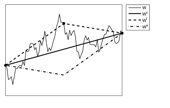
Similarly, we define the corresponding two half-timesteps of the first fine path approximation by
where . Using this relation, the equations for the two fine timesteps can be combined to give an equation for the increment over the coarse timestep,
The antithetic approximation is defined by exactly the same discretisation except that the Brownian increments and are swapped, as illustrated in Figure 1. This gives
and hence
Swapping and does not change the distribution of the driving Brownian increments, and hence has exactly the same distribution as . Note also the change in sign in the last term in (6.2) compared to the corresponding term in (6.2). This is important because these two terms cancel when the two equations are averaged.
These last terms correspond to the Lévy areas for the fine path and the antithetic path, and the sign reversal is a particular instance of a more general result for time-reversed Brownian motion, [30]. If denotes a Brownian motion on the time interval then the time-reversed Brownian motion defined by
| (39) |
has exactly the same distribution, and it can be shown that its Lévy area is equal in magnitude and opposite in sign to that of .
Lemma 6.2.
If , and are as defined above, then
and
In the next section we will see how this lemma generalizes to non-linear multidimensional SDEs (4).
6.3 Milstein discretisation - General theory
Using the coarse timestep , the coarse path approximation , is given by the Milstein approximation without the Lévy area term,
The first fine path approximation (that corresponds to ) uses the corresponding discretisation with timestep ,
where .
The antithetic approximation is defined by exactly the same discretisation except that the Brownian increments and are swapped, so that
It can be shown that [22]
Lemma 6.3.
For all integers , there exists a constant such that
Let’s denote the average fine and antithetic path as follows
The main results of [22] is the following theorem:
Theorem 6.4.
For all , there exists a constant such that
This together with a classical strong convergence result for Milstein discretization allows to estimate the MLMC variance for smooth payoffs. n the case of payoff which is a smooth function of the final state , taking in Lemma 6.1, in Lemma 6.3 and in Theorem 6.4, immediately gives the result that the multilevel variance
has an upper bound. This matches the convergence rate for the multilevel method for scalar SDEs using the standard first order Milstein discretisation, and is much better than the convergence obtained with the Euler-Maruyama discretisation.
However, very few financial payoff functions are twice differentiable on the entire domain . A more typical 2D example is a call option based on the minimum of two assets,
which is piecewise linear, with a discontinuity in the gradient along the three lines , and for .
To handle such payoffs, an assumption which bounds the probability of the solution of the SDE having a value at time close to such lines with discontinuous gradients is needed.
Assumption 6.5.
The payoff function has a uniform Lipschitz bound, so that there exists a constant such that
and the first and second derivatives exist, are continuous and have uniform bound at all points , where is a set of zero measure, and there exists a constant such that the probability of the SDE solution being within a neighbourhood of the set has the bound
In a 1D context, Assumption 6.5 corresponds to an assumption of a locally bounded density for .
Giles and Szpruch in [22] proved the following result
Theorem 6.6.
6.4 Piecewise linear interpolation analysis
The piecewise linear interpolant for the coarse path is defined within the coarse timestep interval as
Likewise, the piecewise linear interpolants and are defined on the fine timestep as
and there is a corresponding definition for the fine timestep . It can be shown that [22]
Theorem 6.7.
For all , there exists a constant such that
where is the average of the piecewise linear interpolants and .
For an Asian option, the payoff depends on the average
This can be approximated by integrating the appropriate piecewise linear interpolant which gives
Due to Hölder’s inequality,
and similarly
Hence, if the Asian payoff is a smooth function of the average, then we obtain a second order bound for the multilevel correction variance.
This analysis can be extended to include payoffs which are a smooth function of a number of intermediate variables, each of which is a linear functional of the path of the form
for some vector function and measure . This includes weighted averages of at a number of discrete times, as well as continuously-weighted averages over the whole time interval.
As with the European options, the analysis can also be extended to payoffs which are Lipschitz functions of the average, and have first and second derivatives which exist, and are continuous and uniformly bounded, except for a set of points of zero measure.
Assumption 6.8.
The payoff has a uniform Lipschitz bound, so that there exists a constant such that
and the first and second derivatives exist, are continuous and have uniform bound at all points , where is a set of zero measure, and there exists a constant such that the probability of being within a neighbourhood of the set has the bound
Theorem 6.9.
We refer the reader to [22] for more details.
6.5 Simulations for antithetic Monte Carlo
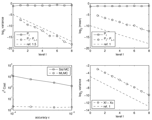
Here we present numerical simulations for a European option for process simulated by , and defined in section 6.2 with initial conditions . The results in Figure 2 are for a European call option with terminal time 1 and strike , that is The top left left plot shows the behaviour of the variance of both and . The superimposed reference slope with rate 1.5 indicates that the variance , corresponding to computational complexity of antithetic MLMC. The top right plot shows that . The bottom left plot shows the computational complexity (as defined in Theorem 2.1) with desired accuracy . The plot is of versus , because we expect to see that is only weakly dependent on for MLMC. For standard Monte Carlo, theory predicts that should be proportional to the number of timesteps on the finest level, which in turn is roughly proportional to due to the weak convergence order. For accuracy , the antithetic MLMC is approximately 500 times more efficient than the standard Monte Carlo. The bottom right plot shows that . This corresponds to standard strong convergence of order 0.5.
We have also tested the algorithm presented in [22] for approximation of Asian options. Our results were almost identical as for European options. In order to treat the lookback, digital and barrier options we found that a suitable antithetic approximation to the Lévy areas are needed. For suitable modification of the antithetic MLMC estimator we performed numerical experiments where we obtained complexity for estimating barrier, digital and lookback options. Currently, we are working on theoretical justification of our results.
7 Other uses of multilevel method
7.1 SPDEs
Multilevel method has been used for a number of parabolic and elliptic SPDE applications [4, 10, 27] but the first use for a financial SPDE is in a new paper by Giles & Reisinger [21].
This paper considers an unusual SPDE which results from modelling credit default probabilities,
| (43) |
subject to boundary condition . Here represents the probability density function for firms being a distance from default at time . The diffusive term is due to idiosyncratic factors affecting individual firms, while the stochastic term due to the scalar Brownian motion corresponds to the systemic movement due to random market effects affecting all firms.
Using a Milstein time discretisation with uniform timestep , and a central space discretisation of the spatial derivatives with uniform spacing gives the numerical approximation
| (44) | |||||
where the are standard Normal random variables so that corresponds to an increment of the driving scalar Brownian motion.
The paper shows that the requirment for mean-square stability as the grid is refined and is , and in addition the accuracy is . Because of this, the multilevel treatment considers a sequence of grids with
The multilevel implementation is very straightforward, with the Brownian increments for the fine path being summed pairwise to give the corresponding Brownian increments for the coarse path. The payoff corresponds to different tranches of a credit derivative that depends on a numerical approximation of the integral
The computational cost increases by factor 8 on each level, and numerical experiments indicate that the variance decreases by factor 16. The MLMC Theorem still applies in this case, with and , and so the overall computational complexity to achieve an RMS error is again .
7.2 Nested simulation
The pricing of American options is one of the big challenges for Monte Carlo methods in computational finance, and Belomestny & Schoenmakers have recently written a very interesting paper on the use of multilevel Monte Carlo for this purpose [5]. Their method is based on Anderson & Broadie’s dual simulation method [1] in which a key component at each timestep in the simulation is to estimate a conditional expectation using a number of sub-paths.
In their multilevel treatment, Belomestny & Schoenmakers use the same uniform timestep on all levels of the simulation. The quantity which changes between different levels of simulation is the number of sub-samples used to estimate the conditional expectation.
To couple the coarse and fine levels, the fine level uses sub-samples, and the coarse level uses of them. Similar research by N. Chen 111unpublished, but presented at the MCQMC12 conference. found the multilevel correction variance is reduced if the payoff on the coarse level is replaced by an average of the payoffs obtained using the first and the second samples. This is similar in some ways to the antithetic approach described in section 6.
In future research, Belomestny & Schoenmakers intend to also change the number of timesteps on each level, to increase the overall computational benefits of the multilevel approach.
7.3 Truncated series expansions
Building on earlier work by Broadie and Kaya [7], Glasserman and Kim have recently developed an efficient method [25] of exactly simulating the Heston stochastic volatility model [29].
The key to their algorithm is a method of representing the integrated volatility over a time interval , conditional on the initial and final values, and as
where are independent random variables.
In practice, they truncate the series expansions at a level which ensures the desired accuracy, but a more severe truncation would lead to a tradeoff between accuracy and computational cost. This makes the algorithm a candidate for a multilevel treatment in which level computation performs the truncation at (taken to be the same for all three series, for simplicity).
To give more details, the level computation would use
while the level computation would use
with the same random variables .
This kind of multilevel treatment has not been tested experimentally, but it seems that it might yield some computational savings even though Glasserman and Kim typically retain only 10 terms in their summations through the use of a carefully constructed estimator for the truncated remainder. In other circumstances requiring more terms to be retained, the savings may be larger.
7.4 Mixed precision arithmetic
The final example of the use of multilevel is unusual, because it concerns the computer implementation of Monte Carlo algorithms.
In the latest CPUs from Intel and AMD, each core has a vector unit which can perform 8 single precision or 4 double precision operations with one instruction. Together with the obvious fact that double precision variables are twice as big as single pecision variables and so require twice as much time to transfer, in bulk, it leads to single precision computations being twice as fast as double precision computations. On GPUs (graphics processors) the difference in performance can be even larger, up to a factor of eight in the most extreme cases.
This raises the question of whether single precision arithmetic is sufficient for Monte Carlo simulation. In general, our view is that the errors due to single precision arithmetic are much smaller than the errors due to
-
•
statistical error due to Monte Carlo sampling;
-
•
bias due to SDE discretisation;
-
•
model uncertainty.
We have just two concerns with single precision accuracy:
-
•
there can be significant errors when averaging the payoffs unless one uses binary tree summation [higham93] to perform the summation;
-
•
when computing Greeks using “bumping”, the single precision inaccuracy can be greatly amplified if a small bump is used.
Our advice would be to always use double precision for the final accumulation of payoff values, and pathwise sensitivity analysis as much as possible for computing Greeks, but if there remains a need for the path simulation to be performed in double precision then one could use two-level approach in which level 0 corresponds to single precision and level 1 corresponds to double precison.
On both levels one would use the same random numbers. The multilevel analysis would then give the optimal allocation of effort between the single precision and double precision computations. Since it is likely that most of the calculations would be single precision, the computational savings would be a factor two or more compared to standard double precision calculations.
8 Multilevel Quasi-Monte Carlo
In Theorem 2.1, if , so that rate at which the multilevel variance decays with increasing grid level is greater than the rate at which the computational cost increases, then the dominant computational cost is on the coarsest levels of approximation.
Since coarse levels of approximation correspond to low-dimensional numerical quadrature, it is quite natural to consider the use of quasi-Monte Carlo techniques. This has been investigated by Giles & Waterhouse [23] in the context of scalar SDEs with a Lipschitz payoff. Using the Milstein approximation with a doubling of the number of timesteps on each level gives and . They used a rank-1 lattice rule to generate the quasi-random numbers, randomisation with 32 independent offsets to obtain confidence intervals, and a standard Brownian Bridge construction of the increments of the driving Brownian process.
Their empirical observation was that MLMC on its own was better than QMC on its own, but the combination of the two was even better. The QMC treatment greatly reduced the variance per sample for the coarsest levels, resulting in significantly reduced costs overall. In the simplest case of a European call option, shown in Figure 3, the top left plot shows the reduction in the variance per sample as the number of QMC points is increased.
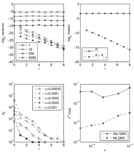
The benefit is much greater on the coarsest levels than on the finest levels. In the bottom two plots, the number of QMC points on each level is determined automatically to obtain the required accuracy; see [23] for the precise details. Overall, the computational complexity appears to be reduced from to approximately .
Giles & Waterhouse interpreted the fact that the variance is not reduced on the finest levels as being due to a lack of significant low-dimensional content. i.e. the difference in the two payoffs due to neighbouring grid levels is due to the difference in resolution of the driving Brownian path, and this is inherently of high dimensionality. This suggests that in other applications with , which would lead to the dominant cost being on the finest levels, then the use of quasi-Monte Carlo methods is unlikely to yield any benefits.
Further research is needed in this area to investigate the use of other low-discrepancy sequences (e.g. Sobol) and other ways of generating the Brownian increments (e.g. PCA). We also refer the reader to [15] for some results for randomized multilevel quasi-Monte Carlo.
9 Conclusions
In the past 6 years, considerable progress has been achieved with the multilevel Monte Carlo method for financial options based on underlying assets described by Brownian diffusions, jump diffusions, and more general Lévy processes.
The multilevel approach is conceptually very simple. In essence it is a recursive control variate strategy, using a coarse path simulation as a control variate for a fine path simulation, relying on strong convergence properties to ensure a very strong correlation between the two.
In practice, the challenge is to couple the coarse and fine path simulations as tightly as possible, minimising the difference in the payoffs obtained for each. In doing this, there is considerable freedom to be creative, as shown in the use of Brownian Bridge constructions to improve the variance for lookback and barrier options, and in the antithetic estimators for multi-dimensinal SDEs which would require the simulation of Lévy areas to achieve first order strong convergence. Another challenge is avoiding large payoff differences due to discontinuous payoffs; here one can often use either conditional expectations to smooth the payoff, or a change of measure to ensure that the coarse and fine paths are on the same side of the discontinuity.
Overall, multilevel methods are being used for an increasingly wide range of applications. This biggest savings are in situations in which the coarsest approximation is very much cheaper than the finest. If the finest level of approaximation has only 32 timesteps, then there are very limited savings to be achieved, but if the finest level has 256 timesteps, then the potential savings are much larger.
Looking to the future, exciting areas for further research include:
-
•
more research on multilevel techniques for American and Bermudan options;
-
•
more investigation of multilevel Quasi Monte Carlo methods;
-
•
use of multilevel ideas for completely new financial applications, such as Gaussian copula and new SPDE models.
References
- [1] L. Andersen and M. Broadie. A primal-dual simulation algorithm for pricing multi-dimensional American options. Management Science, 50(9):1222–1234, 2004.
- [2] A. Asmussen and P. Glynn. Stochastic Simulation. Springer, New York, 2007.
- [3] R. Avikainen. On irregular functionals of SDEs and the Euler scheme. Finance and Stochastics, 13(3):381–401, 2009.
- [4] A. Barth, C. Schwab, and N. Zollinger. Multi-level Monte Carlo finite element method for elliptic PDEs with stochastic coefficients. Numerische Mathematik, 119(1):123–161, 2011.
- [5] D. Belomestny and J. Schoenmakers. Multilevel dual approach for pricing American style derivatives. Preprint 1647, WIAS, 2011.
- [6] M. Broadie, P. Glasserman, and S. Kou. A continuity correction for discrete barrier options. Mathematical Finance, 7(4):325–348, 1997.
- [7] M. Broadie and O. Kaya. Exact simulation of stochastic volatility and other affine jump diffusion processes. 54(2):217–231, 2006.
- [8] S. Burgos and M.B. Giles. Computing Greeks using multilevel path simulation. In L. Plaskota and H. Woźniakowski, editors, Monte Carlo and Quasi-Monte Carlo Methods 2010. Springer-Verlag, 2012.
- [9] J.M.C. Clark and R.J. Cameron. The maximum rate of convergence of discrete approximations for stochastic differential equations. In B. Grigelionis, editor, Stochastic Differential Equations, no. 25 in Lecture Notes in Control and Information Sciences. Springer-Verlag, 1980.
- [10] K.A. Cliffe, M.B. Giles, R. Scheichl, and A. Teckentrup. Multilevel Monte Carlo methods and applications to elliptic PDEs with random coefficients. Computing and Visualization in Science, 14(1):3–15, 2011.
- [11] K. Debrabant, M. B Giles, and A. Rossler. Numerical analysis of multilevel monte carlo path simulation using milstein discretization: scalar case. Technical report, 2011.
- [12] S. Dereich. Multilevel Monte Carlo algorithms for Lévy-driven SDEs with Gaussian correction. Annals of Applied Probability, 21(1):283–311, 2011.
- [13] S. Dereich and F. Heidenreich. A multilevel monte carlo algorithm for lévy-driven stochastic differential equations. Stochastic Processes and their Applications, 2011.
- [14] J.G. Gaines and T.J. Lyons. Random generation of stochastic integrals. SIAM Journal of Applied Mathematics, 54(4):1132–1146, 1994.
- [15] Thomas Gerstner and Marco Noll. Some results for randomized multilevel quasi-Monte Carlo path simulation. Chapter in this book, 2012.
- [16] M.B. Giles. Monte Carlo evaluation of sensitivities in computational finance. Technical Report NA07/12, 2007.
- [17] M.B. Giles. Improved multilevel Monte Carlo convergence using the Milstein scheme. In A. Keller, S. Heinrich, and H. Niederreiter, editors, Monte Carlo and Quasi-Monte Carlo Methods 2006, pages 343–358. Springer-Verlag, 2008.
- [18] M.B. Giles. Multilevel Monte Carlo path simulation. Operations Research, 56(3):607–617, 2008.
- [19] M.B. Giles. Multilevel Monte Carlo for basket options. In Proceedings of the Winter Simulation Conference 2009, 2009.
- [20] M.B. Giles, D.J. Higham, and X. Mao. Analysing multilevel Monte Carlo for options with non-globally Lipschitz payoff. Finance and Stochastics, 13(3):403–413, 2009.
- [21] M.B. Giles and C. Reisinger. Stochastic finite differences and multilevel Monte Carlo for a class of SPDEs in finance. SIAM Journal of Financial Mathematics, to appear, 2012.
- [22] M.B. Giles and L. Szpruch. Antithetic Multilevel Monte Carlo estimation for multi-dimensional SDEs without Lévy area simulation. Arxiv preprint arXiv:1202.6283, 2012.
- [23] M.B. Giles and B.J. Waterhouse. Multilevel quasi-Monte Carlo path simulation. In Advanced Financial Modelling, Radon Series on Computational and Applied Mathematics, pages 165–181. de Gruyter, 2009.
- [24] P. Glasserman. Monte Carlo Methods in Financial Engineering. Springer, New York, 2004.
- [25] P. Glasserman and K.-K. Kim. Gamma expansion of the Heston stochastic volatility model. Finance and Stochastics, 15(2):267–296, 2011.
- [26] P. Glasserman and N. Merener. Convergence of a discretization scheme for jump-diffusion processes with state-dependent intensities. Proc. Royal Soc. London A, 460:111–127, 2004.
- [27] S. Graubner. Multi-level Monte Carlo Methoden für stochastiche partial Differentialgleichungen. Diplomarbeit, TU Darmstadt, 2008.
- [28] S. Heinrich. Multilevel Monte Carlo Methods, volume 2179 of Lecture Notes in Computer Science, pages 58–67. Springer-Verlag, 2001.
- [29] S.I. Heston. A closed-form solution for options with stochastic volatility with applications to bond and currency options. Review of Financial Studies, 6:327–343, 1993.
- [30] I. Karatzas and S.E. Shreve. Brownian Motion and Stochastic Calculus. Graduate Texts in Mathematics, Vol. 113. Springer, New York, 1991.
- [31] A. Kebaier. Statistical Romberg extrapolation: a new variance reduction method and applications to options pricing. Annals of Applied Probability, 14(4):2681–2705, 2005.
- [32] P. Kloeden and A. Neuenkirch. Convergence of numerical methods for stochastic differential equations in mathematical finance. Chapter in this book, 2012.
- [33] P.E. Kloeden, A. Neuenkirch, and R. Pavani. Multilevel monte carlo for stochastic differential equations with additive fractional noise. Annals of Operations Research, pages 1–22, 2011.
- [34] P.E. Kloeden and E. Platen. Numerical Solution of Stochastic Differential Equations. Springer, Berlin, 1992.
- [35] X. Mao and L. Szpruch. Strong convergence rates for backward euler–maruyama method for non-linear dissipative-type stochastic differential equations with super-linear diffusion coefficients. Stochastics, 2012.
- [36] R.C. Merton. Option pricing when underlying stock returns are discontinuous. Journal of Finance, 3:125–144, 1976.
- [37] T. Müller-Gronbach. The optimal uniform approximation of systems of stochastic differential equations. The Annals of Applied Probability, 12(2):664–690, 2002.
- [38] T. Müller-Gronbach. Strong approximation of systems of stochastic differential equations. Habilitation thesis, TU Darmstadt, 2002.
- [39] G. Pagès. Multi-step Richardson-Romberg extrapolation: remarks on variance control and complexity. Monte Carlo Methods and Applications, 13(1):37–70, 2007.
- [40] E. Platen and N. Bruti-Liberati. Numerical Solution of Stochastic Differential Equations With Jumps in Finance. Springer, 2010.
- [41] T. Rydén and M. Wiktorsson. On the simulation of iterated Itô integrals. Stochastic Processes and their Applications, 91(1):151–168, 2001.
- [42] A.L. Speight. A multilevel approach to control variates. Journal of Computational Finance, 12:1–25, 2009.
- [43] A.L. Speight. Multigrid techniques in economics. Operations Research, 58(4):1057–1078, 2010.
- [44] L. Szpruch, X. Mao, D.J. Higham, and J. Pan. Numerical simulation of a strongly nonlinear ait-sahalia-type interest rate model. BIT Numerical Mathematics, 51(2):405–425, 2011.
- [45] M. Wiktorsson. Joint characteristic function and simultaneous simulation of iterated Itô integrals for multiple independent Brownian motions. Annals of Applied Probability, 11(2):470–487, 2001.
- [46] Y. Xia. Multilevel Monte Carlo method for jump-diffusion SDEs. Arxiv preprint arXiv:1106.4730, 2011.
- [47] Y. Xia and M.B. Giles. Multilevel path simulation for jump-diffusion SDEs. In L. Plaskota and H. Woźniakowski, editors, Monte Carlo and Quasi-Monte Carlo Methods 2010. Springer-Verlag, 2012.