Phase diagram of the Asymmetric Hubbard Model and an entropic chromatographic method for cooling cold fermions in optical lattices

Abstract

We study the phase diagram of the asymmetric Hubbard model (AHM), which is characterized by different values of the hopping for the two spin projections of a fermion or equivalently, two different orbitals. This model is expected to provide a good description of a mass-imbalanced cold fermionic mixture in a 3D optical lattice. We use the dynamical mean field theory to study various physical properties of this system. In particular, we show how orbital-selective physics, observed in multi-orbital strongly correlated electron systems, can be realized in such a simple model. We find that the density distribution is a good probe of this orbital selective crossover from a Fermi liquid to a non-Fermi liquid state. Below an ordering temperature $T_{o}$, which is a function of both the interaction and hopping asymmetry, the system exhibits staggered long range orbital order. Apart from the special case of the symmetric limit, i.e., Hubbard model, where there is no hopping asymmetry, this orbital order is accompanied by a true charge density wave order for all values of the hopping asymmetry. We calculate the order parameters and various physical quantities including the thermodynamics in both the ordered and disordered phases. We find that the formation of the charge density wave is signaled by an abrupt increase in the sublattice double occupancies. Finally, we propose a new method, entropic chromatography, for cooling fermionic atoms in optical lattices, by exploiting the properties of the AHM. To establish this cooling strategy on a firmer basis, we also discuss the variations in temperature induced by the adiabatic tuning of interactions and hopping parameters.

I Introduction

Strongly correlated electronic systems are known to exhibit a wide variety of interesting and novel phases ranging from Fermi liquids, heavy fermions, Mott insulators, superconductors to other states with complex long range orders. The field of strongly correlated fermions in condensed matter shares many common research goals with that of cold atoms loaded in optical lattices. Yet these two fields emerge from different scientific communities and often look at similar problems with different tools and from different physical perspectives. In this context, the present theoretical study focuses on a model hamiltonian that generalizes central models of strongly correlated electron systems, which, nevertheless, might only be experimentally realized with cold atoms in an optical lattice. The present work is a contribution towards building bridges between these two scientific communities.

The paradigmatic model of correlated fermions is the Hubbard modelHubbard (1963) (HM), which describes itinerant electrons on a lattice with hopping $t$ and subjected to an onsite repulsion $U$ stemming from screened Coulomb interactions between two electrons. This model, though the focal point of interest in condensed matter physics for decades, however remains unsolved in two and three spatial dimensions. In the limit of infinite dimensions, or infinite lattice connectivity, the model remains non-trivial but is exactly solvable using the dynamical mean field theory (DMFT)Georges et al. (1996). DMFT shows that in the absence of any frustration, the ground state of the system at half-filling is an antiferromagnetic insulator for all values of $U$ with an associated Néel temperature. In cases where due to inherent frustration the system is in a paramagnetic state, one finds a correlated metal described by a Fermi liquid with heavy quasiparticles at low and moderate $U$. Upon increasing the interaction strength, always at half-filling, the heavy metal breaks down and a Mott insulating state is realized with a coexistence region Georges et al. (1996). Such a Mott transition was indeed observed in the classic three dimensional Mott-Hubbard system V₂O₃ Georges et al. (1996).

Another important model Hamiltonian of strongly correlated systems is the Falicov-Kimball modelFalicov and Kimball (1969) (FKM), which is a simplified variant of the HM where one of the spin species has zero hopping, hence, its motion is frozen. This model explicitly breaks the spin SU(2) symmetry and DMFT studies Freericks and Zlatić (2003) showed that it has an antiferromagnetically ordered insulating phase at half-filling, and regions of phase separation at low values of the onsite Coulomb interaction for finite doping. Similar to the HM, a paramagnetic Mott metal -insulator transition (without any coexistence) as a function of the interaction strength was also found in the FKM at half filling. A fundamental difference between the two models is that while the metallic state in the HM was described by a Fermi liquid, the metallic state in the FKM is a non-Fermi liquid with no quasiparticles. This exotic state stems from the broken translational symmetry due to the random distributions of the immobile electrons on the lattice. Georges et al. (1996); Si et al. (1992); Freericks and Zlatić (2003).

The natural connection between these two models is the Asymmetric Hubbard model (AHM), where each spin species has a different hopping amplitude. This model, originally considered purely academic in solid state systems, is of particular relevance to cold atoms on optical lattices. In fact, asymmetric Hubbard models are realizable in optical lattices, using either two hyperfine states of a spin-$1/2$ atom or two different spinless fermionic atoms (e.g., ${}^{6}\mathrm{Li}$ and ${}^{40}\mathrm{K}$), as described in Refs. Mandel et al., 2003; Taie et al., 2010; Bloch et al., 2008; Cazalilla et al., 2005; Wang et al., 2009; Dao et al., 2007; Lin et al., 2006. Each of the hopping amplitudes $t_{\sigma}$ can be independently controlled by changing the intensity of the lasers and the Coulomb interaction strength $U$ is related to the scattering length and can be well controlled by Fano-Feshbach resonanceWille et al. (2008); Chin et al. (2010). Following Refs. Nascimbène et al., 2010; Dao et al., 2012, the hopping asymmetry $r$ in a mixture of ${}^{6}\mathrm{Li}$/${}^{40}\mathrm{K}$ can be tuned from values close to the FKM (r=0) to that of the HM (r=1).

Another important reason to study the AHM, is the fact that it can be thought of as a minimal model of multi-orbital systems. Earlier multi-orbital models in (bosonic) cold-atom systems have been considered in Refs. Alon et al., 2005; Scarola and Das Sarma, 2005; Isacsson and Girvin, 2005. In general, in correlated materials, often when there is more than one band close to the Fermi energy, new physical phenomena arise. The existence of many interacting bands close to the Fermi energy, may generate exotic phases, produced by the difference in the population of each band, the inter and intra band Coulomb interaction, as well as the Hund’s coupling. Examples of these materials, which are subjects of current research include high-T${}_{\textrm{c}}$ iron-based superconductors, where 5 bands cross the Fermi energy. From this perspective, the AHM, which can be viewed as a model for spinless fermions with two different orbitals, can be considered as an attempt to approach the physics of correlated multi-orbital systems, in cold-atoms. For this reason, in this paper we adopt the notation of two different orbitals $h$ and $l$, instead of two spin-projections $\uparrow$ and $\downarrow$, as we will explain later.

Most of the recent theoretical work on the AHM in the cold-atoms context, has concentrated on establishing the phase diagram in the one dimensional case, for both, attractive and repulsive interactions. A rich variety of groundstates have been found, including Mott insulator, charge density wave and superconductivity, in the case of mixtures of equal density Cazalilla et al. (2005), and also FFLO states in the case of population imbalance Wang et al. (2009). Beyond the one dimensional case, the AHM with attractive interactions on a cubic optical lattice, has been studied using DMFT Dao et al. (2007). A related, but more general model, was also analyzed in Ref. Brydon, 2008 using the slave-boson technique. The phase diagram of the repulsive AHM without any long-range order was studied using DMFT in Refs.Winograd et al., 2011; Dao et al., 2012. Both studies found a Mott transition with a region of two coexistent solutions, at low enough temperatures for all non-zero values of the hopping asymmetry. In particular, in Ref.Winograd et al., 2011, we showed that an interesting temperature driven orbital-selective crossover takes place in the AHM. At temperatures below a coherence temperature $T_{coh}$, the system is a heavy Fermi-liquid, qualitatively analogous to the Fermi liquid state of the symmetric Hubbard model. Above $T_{coh}$, instead of the standard incoherent metal seen in the HM case, an orbital-selective crossover occurs, wherein one fermionic species effectively localizes, and the metallic state maps onto the non-Fermi liquid of the Falicov-Kimball model. This is a validation of the fact that the AHM can be considered as a minimal model for the study of orbital physics. Various observables such as the double occupation, the specific heat and entropy were also computed. As stated earlier, a phase diagram without any long-range order is appropriate provided an inherent frustration prevents the formation of any kind of orbital ordering. However, for the unfrustrated case, which corresponds to the bare model hamiltonian without additional assumptions, one needs to explore ordered solutions to the mean field equations. Here, for simplicity, we restrict ourselves to the case of half-filling, where only Néel-type (ie checkerboard) order is realized. However, away from half-filling, incommensurate order may also occur Freericks and Zlatić (2003); Camjayi et al. (2007). To explore the long-range ordered solutions and to understand the way how these are connected to the previously studied finite temperature crossover regimes, including the orbital selective stateWinograd et al. (2011), is the main goal of the present work. In this paper, we study the orbital-ordered phases as a function of hopping asymmetry, interaction strength and temperature, which then permits us to obtain a complete phase diagram of the half-filled AHM. Since fermionic cold atom systems have not yet attained the low temperatures which are requisite for observing any kind of order, we also propose a novel cooling scheme which is based on the hopping asymmetry of the two orbitals.

The present problem is at the interface between two different fields, thus, we summarize all the technical details in a self-contained section II.1 that can be skipped if desired. For further information on the DMFT-technique we suggest Ref. Georges et al., 1996. Qualitative features of the long-range order phase are described in II.2. In section III.1, we briefly review the results of the disordered phase of the AHM found in Ref. Winograd et al., 2011, and discuss their consequences for cold atoms experiments. In section III.2, we discuss the ordered phase of the AHM and present results for the critical temperature $T_{o}$ , the different order parameters and the thermodynamical quantities of the model. In section III.3, we propose a strategy for cooling down a mixture of cold fermionic atoms, that exploits the mass imbalance and may have practical applications. In section III.4, we analyze the effects on the temperature of the condensate of tuning the values of hopping and interaction of the atomic particles. Finally in section IV, we summarize our conclusions. The expressions used to compute the physical observables can be found in the appendix.

II Model and Method

II.1 Mean-field equations

The asymmetric Hubbard model Hamiltonian reads,

$$H=-\sum_{<i,j>;\sigma=l,h}t_{\sigma}c_{i\sigma}^{\dagger}c_{j\sigma}^{\phantom{{\dagger}}}+U\sum_{i}(n_{il}-1/2)(n_{ih}-1/2)$$ (1)

where $c^{\dagger}_{i\sigma},c_{i\sigma}$ are the fermion creation and annihilation operators at site $i$ and $\sigma=l,h$ labels the two orbitals, light and heavy. $t_{\sigma}$ and $U$ denote the hopping and the repulsive interaction strengths and the asymmetry parameter is defined as $r$=$t_{h}/t_{l}$. The limits $r$=0 and $r$=1 correspond to the FKM and HM, respectively. We restrict our study to the particle-hole symmetric half-filled case, with number of particles per site $\langle n_{l}\rangle=\langle n_{h}\rangle=1/2$. To describe a realization of the AHM in cold atom systems in an optical lattice, one would need to add a confining potential to the hamiltonian (1). For simplicity, in this initial study, we do not include any confining potential in our hamiltonian. Nevertheless, based on previous results obtained for the Hubbard model within the LDA or R-DMFT treatment including the trapping potential Dao et al. (2007); Gorelik et al. (2010), we expect our results to be reliable for the bulk of the optical lattice. The confinig potential typically affects the sites in a thin outer shell of the lattice, with a thickness of only a few sitesGorelik et al. (2010).

We now briefly discuss the DMFT method used to study the AHM. This method, which is exact in the limit of infinite lattice coordination, relies on a mapping of the present problem onto a quantum impurity problem subject to self-consistency conditions. Here we consider the AHM on a Bethe lattice characterized by the semi-circular density of states,

$$\rho_{\sigma}(\epsilon)=\frac{2}{\pi D_{\sigma}}\sqrt{1-(\epsilon/D_{\sigma})^{2}}$$ (2)

with $D_{\sigma}=2t_{\sigma}$. We set $D_{l}\equiv D=1$ as the unit of energy in what follows. The advantage of the Bethe lattice is that it provides numerical simplifications and also is expected to yield accurate estimates for a 3D simple-cubic latticeGeorges et al. (1996), adopting $D_{\sigma}=6t_{\sigma}$.

We solve the DMFT equations using two standard numerical methods: the Hirsch-Fye quantum Monte Carlo algorithm (HF-QMC), which is exact in the statistical sense; and the exact diagonalization method (ED), which is in principle exact and whose discretization errors can be systematic reduced. Their implementation is described in detail in Ref. Georges et al., 1996. The use of these two different methods further provides a crosscheck of our numerical results.

To obtain a complete phase diagram of the AHM, we need to consider both ordered and disordered solutions to the dynamical mean field equations. We discuss the two cases below.

II.1.1 Disordered solution

In the disordered phase, the system can be mapped onto a quantum impurity problem described by the imaginary time effective action:

$$\textrm{S}_{\textrm{eff}}=-\int_{0}^{\beta}d\tau\int_{0}^{\beta}d\tau^{\prime}\sum_{\sigma=l,h}c^{\dagger}_{\sigma}(\tau)\mathcal{G}_{0\sigma}^{-1}(\tau-\tau^{\prime})c_{\sigma}(\tau^{\prime})+U\int_{0}^{\beta}d\tau(n_{l}(\tau)-1/2)(n_{h}(\tau)-1/2)$$ (3)

The retarded Green’s function $\mathcal{G}_{0\sigma}$ is related to the full local Green’s function $G_{\sigma}$ through the following self consistency conditions,

$$\mathcal{G}_{0\sigma}^{-1}(i\omega_{n})=i\omega_{n}+\mu_{\sigma}-t_{\sigma}^{2}G_{\sigma}(i\omega_{n})$$ (4)

$\omega_{n}$ are the Matsubara frequencies and $\mu_{\sigma}$ are the chemical potentials for the two species. At the self consistent point, the impurity and the lattice local Green’s functions coincide. Therefore, the Eqs. (3) and (4) can be simply solved by direct substitution. Note that unlike the HM case, here the disordered phase is characterized by two self-consistent equations because the AHM explicitly breaks orbital rotational invariance for all $r\neq 1$.

II.1.2 Checkerboard-like ordered solution

Given that both the HM and the FKM realize phases with long range order, we expect the AHM to also have such phases. Based on the nature of the known solutions of the aforementioned models, here, we assume a checkerboard-like order for the AHM, as well. This implies the existence of two sublattices $A$ and $B$ such that each site of sublattice $A$ is connected only to the sites of sublattice $B$ and viceversa. In the AHM, the existence of two inequivalent sites necessitates a mapping onto two impurity models similar to the one described in (3) and the respective Green’s functions obey the following self consistency conditions,

$$\mathcal{G}_{0\sigma A}^{-1}(i\omega_{n}) = i\omega_{n}+\mu_{\sigma}-t_{\sigma}^{2}G_{\sigma B}(i\omega_{n})$$

$$\mathcal{G}_{0\sigma B}^{-1}(i\omega_{n}) = i\omega_{n}+\mu_{\sigma}-t_{\sigma}^{2}G_{\sigma A}(i\omega_{n})$$ (5)

In the limits $r=0,1$, this set of four equations reduces to two. For the case of general asymmetry $(0\leq r<1)$, one needs to deal with the four different self-consistency conditions, which make the problem of the AHM considerably harder. Technically, we have to simultaneously solve two different quantum impurity problems, with two different effective baths each. Solutions with incommensurate order which might exist in this model, especially away from half-fillingFreericks and Jarrell (1995); Freericks (1993); Camjayi et al. (2007) are not considered in this paper. From the structure of the mean-field equations Eqs. II.1.2, we find that for checkerboard-like order at half-filling, the Green’s functions obey the following constraints:

$$\rm{Re}G_{A\sigma}(i\omega_{n}) = -\rm{Re}G_{B\sigma}(i\omega_{n})$$

$$\rm{Im}G_{A\sigma}(i\omega_{n}) = \rm{Im}G_{B\sigma}(i\omega_{n})$$ (6)

We term this symmetry broken state as one with orbital order (OO), and, in the symmetric case for r=1 it coincides with the familiar Néel antiferromagnetic state.

From Eqs.(II.1.2) and (II.1.2), we see that unlike the simpler case of the HM ($r=1$) , here $G_{Al}$ and $G_{Bh}$ can be different for generic values of r$\neq$1. This implies the possibility of a charge density wave (CDW) order, as we shall show below.

II.2 Long-range order phase

Restricting ourselves to the half filled case with equal numbers of light and heavy particles, we find that in the orbitally ordered phase, the average occupations of different orbitals on the A and B sublattices satisfy the constraint $n_{Al}+n_{Bl}=n_{Ah}+n_{Bh}=1$. This implies that

$$n_{Al}-n_{Ah}=-(n_{Bl}-n_{Bh})$$ (7)

Additionally, the sublattice occupation $n_{\alpha}=n_{\alpha l}+n_{\alpha h}$ ($\alpha=A,B$) satisfies the relation

$$-\left(1-n_{A}\right)=1-n_{B}$$ (8)

Eq. (7) indicates that the orbital polarization in sublattice $A$ is the opposite to that of $B$. The order parameter can now be defined as $m_{o}$$=\langle n_{\alpha l}-n_{\alpha h}\rangle/2$, with, $\alpha$ being either $A$ or $B$. In the HM limit, this orbital order translates into a spin density wave with Néel antiferromagnetic order, and $m_{o}$ is the familiar staggered magnetization.

Note that Eq. (8) indicates that orbital ordering coexists with a charge density wave formation in which one sublattice has increased its occupation with respect to the other. The CDW order parameter can be defined as $m_{c}$$=\langle n_{A}-n_{B}\rangle/2$. We see that we have CDW order for all r$\neq$1. In the limit of the HM, both $l$ and $h$ orbitals are equivalent, SU(2) symmetry is recovered and CDW order is lost, since $n_{Al}=n_{Bh}$ and orbital order translates to Néel antiferromagnetic order. An OO with a CDW, in contrast, is realized in the FKM limitFreericks and Zlatić (2003). On heating, these ordered phases survive upto a certain critical temperature $T_{o}$, which coincides with the Néel temperature in the HM, and with the $T_{\textrm{CDW}}$ in the FKM case. To help visualize the variety of states, we sketch in Fig. 1, the different phases as a function of the interactions and the hopping asymmetry.

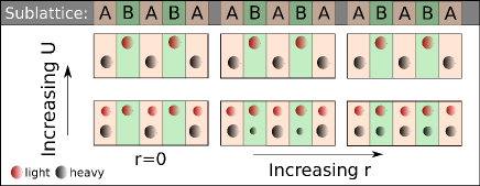
Figure 1: Sketch of different ordered solutions of the AHM. Black (lower) dots, represent particles in the heavy band, while red (upper) dots represent those in the light-one. Bigger dots represent higher occupation. In the SU(2) symmetric point $r\rightarrow 1$ (right-most pannels), only orbital order is possible, and orbital polarization increases with $U$. As $r$ decreases, CDW ($n_{A}\not=n_{B}$) coexists with orbital order (lower left and central panel). CDW formation, nevertheless, decreases with increasing interactions (top panels), since in the Mott insulating state, double occupied sites are energetically unfavorable.

III Results

We now solve the relevant impurity problem with the associated self-consistency condition in both the ordered and the disordered phases, using exact diagonalization and quantum Monte Carlo methods Georges et al. (1996). The use of both methods allows us to crosscheck the results and also obtain the finite temperature phase diagram in the whole relevant parameter range of the model. In Fig. 2, we plot the finite-$T$ Matsubara local Green’s functions for different values of the parameters $U$ and $r=$$t_{h}/t_{l}$  for $T/D$=$D/\beta$=$0.025$. Although detailed features like the densities of states are technically difficult to extract from the Matsubara Green’s functions, some basic properties can be readily obtained. For instance, the extrapolated value of $G(i\omega_{n}\to 0)$ yields the density of states at the Fermi energy, which is expected to be finite in a metal, while it goes to zero in an insulator at low temperatures. This qualitative feature can be observed in the solutions for the disordered (ordered) phase shown in the left (right) panels of Fig. 2 for various values of $r$ and the interaction $U$. This feature allows us to pinpoint the precise location of the metal-insulator transition in the model. Moreover, within DMFT, if the metallic solution is a normal Fermi liquid, it can be shown that the density of states at the Fermi energy at $T=0$ for any $U$, remains pinned at the $U=0$ value Georges et al. (1996). Consequently, if the extrapolated value of the Green’s function does not go to zero (i.e., is not an insulator), but violates the pinning condition, then the self-energy would be non-vanishing at $\omega_{n}\to 0$, hence the states have a finite lifetime, and the solution corresponds to a non-Fermi liquid metallic state. All of these features, coupled with the estimation of various order parameters, help us obtain an interesting and rich finite temperature phase diagram for the AHM.

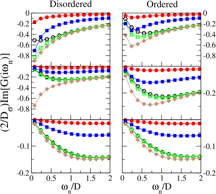
Figure 2: $\textrm{Im}G(i\omega_{n})$ for $T/D=0.025$. The left (right) column corresponds to the disordered (ordered) solution for $U=D,2D,3.5D$, for the first, second and third rows, respectively. Empty (filled) symbols correspond to the light (heavy)-orbital, while circles, squares and diamonds correspond to $r=0.1,0.4,1$, respectively. For the ordered state, note that as shown in Eq. II.1.2, $\textrm{Im}G(i\omega_{n})$ is independent of the sublattice.

III.1 Disordered phase

III.1.1 Phase diagram

The disordered phase of the AHM, has been discussed in detail in recent publications (Refs. Winograd et al., 2011; Dao et al., 2012). Here, for completeness and to facilitate the ensuing discussion, we briefly summarize the main features of the disordered phase diagram. It is schematically shown in Fig. 3 for a generic value of the mass asymmetry parameter $r$. This phase diagram would be appropriate for a fully frustrated system.

At low T, there exists a metal-insulator transition from a metal to a Mott insulator as one increases the repulsion $U$. The metallic phase is characterized by a Fermi liquid for all $r\neq 0$ and generically has two kinds of quasiparticles with different masses. The light particles are more strongly renormalized, since the screening potential produced by the heavy ones is less efficient due to its lower mobility. Despite the different mass renormalization, both quasiparticles disappear (their mass renormalization diverges) at a single critical $U=U_{c2}$, signaling the metal-insulator transition. On the other hand, if one starts at high values of the intereaction $U$, well in the Mott state, and progresively decreases the strength, the insulating gap decreases, and eventually closes. At that point there is an insulator to metal transition, which is denoted as $U_{c1}$. In between these two critical values, one finds a coexistence regime, with two solutions, one insulating and one metallic, as depicted in Fig. 3. The coexistence region extends in temperature from $T$=0 up to finite temperatures. Both solutions are thermodynamically stable within the disordered phase, thus the metal-insulator transition is first order at finite $T$ and culminates in a second order critical point, similarly to the HM caseGeorges et al. (1996). The critical values of the interactions and the $T$-value of the critical end point of this regime, i.e., the area of coexistence, decrease with decreasing $r$.

At lower $U$, the metallic Fermi liquid state survives upto a coherence temperature $T_{coh}(U,r)$. Above $T_{coh}$, the system crosses over to an orbital selective metallic phase, which closely resembles the corresponding non-Fermi liquid state of the FKM model. This intermediate temperature regime, can be thought of as if the hopping of the heavy particles were effectively renormalized to zero, hence becoming localized, while the light ones remain mobile. Orbital selective crossovers between qualitatively different metallic phases, though commonly observed in real materials, such as high-Tc pnictides, heavy fermions, etc., are often not well understood. In this context, our model may be viewed as a minimal model for a non-Fermi liquid state emerging from an orbital-selective mechanism.

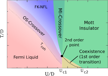
Figure 3: Schematic $T-U$ phase diagram for a generic value of the parameter $r$ Winograd et al. (2011). At low $T$ there are three distinct regimes: a Fermi-liquid state with two different quasiparticles; a coexistence zone, and a Mott insulating phase. In the metallic regime, above $T_{coh}$ there is a crossover to a Falicov-Kimball-like non-Fermi liquid state. Increasing interactions from this phase, the system crosses over to a bad insulating state (a finite $T$ Mott insulator).

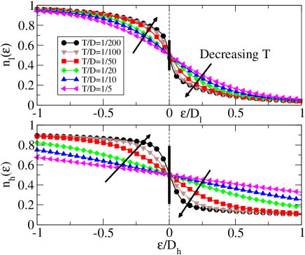
Figure 4: Density distributions of the light and heavy orbitals for $r=0.2$ and $U/D=0.8$. As $T$ decreases, $n(\epsilon)$ tends to the usual Fermi-liquid distributions where there is a discontinuity at the Fermi energy (black arrows show the tendence of $n(\epsilon)$ as $T$ reduces). The vertical black line at $\epsilon=0$ shows the expected jump at $T=0$.

III.1.2 Momentum dependent density of states

Since the AHM is more generic than the Hubbard model, it may be easier to realize in cold fermionic mixtures. Moreover, from the previous discussion it should be clear that the AHM presents the tantalizing possibility of realizing non-Fermi liquid states at relatively high temperatures. These types of poor metallic states are central to many open problems in condensed matter physics. This immediately raises the question of what would be a measurable physical quantity, which is sensitive to the orbital selective crossover to the non-Fermi liquid state.

One practical probe would be time-of-flight experiments Bloch et al. (2008), where the momentum resolved density distribution $n(k)$ is measured. In a conventional Fermi-liquid at zero temperature, $n(k)$ has a jump of size $Z\leq 1$ at the Fermi momentum $k_{F}$, with $Z$ being the quasiparticle residue. Replacing the momentum by the single particle energy $\epsilon$, the resulting quantity $n(\epsilon)$, which is more easily obtained within DMFT, would also exhibit the same jump at the Fermi energy $\epsilon=\epsilon_{F}$. At nonzero $T$, the discontinuity in $n$ is smeared within an energy scale given by $T$ (see Fig. 4). In a non-Fermi liquid state, $Z=0$, and there is no discontinuity even at $T=0$.

Since the crossover of the AHM is at finite $T$, we do not expect to see sharp changes in the density distribution. Nonetheless, going from the HM towards the FKM (reducing $t_{h}/t_{l}$ and keeping all other variables constant), $n(\epsilon)$ evolves to $n^{\textrm{FKM}}(\epsilon)$, for $r<r_{crit}$. However, we find that the slope of $n_{l}(\epsilon)$ at the Fermi energy, as a function of $T^{-1}$ is a better magnitude to pinpoint this crossover. We plot the slope in Fig. 5 and we clearly see that above a certain temperature $T_{\rm OS}$, which depends on $r$ and $U$, $\frac{\partial n^{\textrm{AHM}}}{\partial\epsilon}$ approaches $\frac{\partial n^{\textrm{FKM}}}{\partial\epsilon}$. Therefore, this signals that the light orbital of the AHM evolves to the non-Fermi liquid state of the FKM once orbital-selective crossover has been achieved.

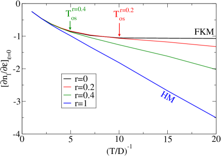
Figure 5: Slope of the light particles density distribution as a function of $(T/D)^{-1}$, for $U/D=0.8$. For $T>T_{\rm OS}$, the metallic behavior of the AHM, coincides with the non-Fermi liquid metallic state of the FKM. For this value of $U$, $T_{\rm OS}(r=0.4)\simeq 0.2D$ and $T_{\rm OS}(r=0.2)\simeq 0.1D$.

III.2 Ordered phase

In the non-frustrated case, we expect the system to order at low temperatures. Solving the equations discussed in section II.1.2, we obtain the critical temperature $T_{o}(r,U)$, below which the orbital order sets in, and the behavior of the order parameters $m_{o}$ and $m_{c}$, defined before.

III.2.1 Ordering Temperature $T_{o}$

We find that analogous to the HM and FKM, at $T=0$ and for all $U\neq 0$, the system is an insulator with long-range order which vanishes above a critical temperature $T_{o}(U,r)$. The results are shown in Fig. 6 for a generic value of $r$=0.4. For comparison, in the figure we also show the main features of the phase diagram discussed before, in Fig. 3. We observe that the metal-insulator transition, described in section III.1 is shadowed by the OO phase, which is thermodynamically more stable. This behaviour is similar to the one realized in the Hubbard model Georges et al. (1996). It is interesting to observe that both the coexistence region, the orbital-selective thermal crossover and the maximum in the orbital ordering temperature $T_{o}$, all occur at the same parameter region, where the interaction $U$ is comparable to the model bandwidth $2D$ and the correlation effects are strongest.

Within DMFT, the simplest procedure to compute the critical temperature $T_{o}$ is to start at low $T$, where the converged DMFT solution is found to have orbital long-range order (i.e., $m_{o}$$\not=0$, see eq. 7) and then slowly increase the temperature until the order vanishes at some $T=T_{o}(r,U)$. We note that these transitions though continuous and second order, are rather sharp as can be seen in Fig. 7, that shows the order parameter $m_{o}$($T$), for $U=D$ and several values of the hopping ratio $r$. In Fig. 8, we plot the ordering temperature as a function of both, the interaction $U$ and hopping asymmetry $r$.

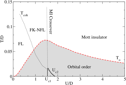
Figure 6: $T$-$U$ phase diagram for $r=0.4$. $T_{o}$ (red dashed line) is the critical temperature. Orbital ordering shadows the metal-insulator transition, which occurs at $T<T_{o}$, like in the case of the HMGeorges et al. (1996). The different phases of the disordered solutions are described in Fig. 3

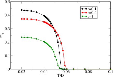
Figure 7: Orbital order parameter $m_{o}$ for different values of the asymmetry $r$ and $U=D$.

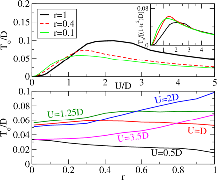
Figure 8: Critical temperature $T_{o}$ as a function of interaction $U$ (upper panel) and hopping ratio $r$ (bottom panel). The scaling $T_{o}\propto(1+r^{2})$ at strong coupling, is shown in the inset of the upper panel.

At weak coupling i.e., small $U$ and for all $r\neq 0$, we see an exponential behaviour , $T_{o}\propto\exp(-c/U)$, where $c$ is some constant, similar to the Hartree mean field result for the Hubbard modelvan Dongen (1991). In the FK limit, we expectvan Dongen and Vollhardt (1990) $T_{o}\propto(U/D)^{2}\ln(D/U)$. The qualitative dependence of $T_{o}$ on $r$ can be understood by considering the competition between kinetic and Coulomb energy. In the disordered metallic region, when $U=0$, $T_{o}$ goes to zero, and there is no order. In the HM, as $U$ increases, the ratio between potential and kinetic energy ($E_{p}/E_{k}$) increases, and so does $T_{o}.$Georges et al. (1996) Since a decreasing $r$ decreases $E_{k}$, the ratio $E_{p}/E_{k}$ and hence $T_{o}$ increase as $r$ decreases in accordance with Fig. 8.

To understand the non-monotonic behaviour of $T_{o}$ seen in the Mott insulating side of the phase diagram, it is useful to consider the large-$U$ limit, where the AHM can be mappedFáth et al. (1995) onto a spin-$1/2$ anisotropic Heisenberg (XXZ) model described by the effective hamiltonian,

$$H_{spin}=J\sum_{<ij>}[\sigma^{x}_{i}\sigma^{x}_{j}+\sigma^{y}_{i}\sigma^{y}_{j}+\gamma(\sigma^{z}_{i}\sigma^{z}_{j}-1)]$$ (9)

with exchange constants $J=$$t_{l}$$t_{h}$$/U$ and $\gamma=\frac{t_{l}^{2}+t_{h}^{2}}{2t_{h}t_{l}}$. This model interpolates between the isotropic Heisenberg model at $r=1$ and the Ising model at $r=0$. A mean field study of this spin model shows us that the ordering temperature $T_{o}$ in the large $U$ limit is proportional to $J\gamma\propto(1+r^{2})$ consistent with the DMFT results, which show that $T_{o}$ decreases with decreasing $r$ in the large $U$ limit (see inset of Fig. 8). This feature also persists in the intermediate $U$ regime as shown in the lower panel of Fig. 8. Therefore, from the previous discussion, the non-monotonic behaviour of $T_{o}$ seen in Fig. 8 is a consequence of the increasing dependence of the ordering $T$ with $U$ at weak coupling, on one hand; and of the decreasing dependence at strong coupling due to the super-exchange interaction, on the other.

III.2.2 Orbital and charge order

We now discuss the orbital and CDW ordering seen in the ordered phase for $T<T_{o}$. In Fig. 9, we plot the order parameter $m_{o}$ (defined in sec. II.2) as a function of the asymmetry $r$ for different values of the interaction, at a fixed finite low $T$. The variation of $m_{o}$ with $r$ is rather complex and depends on the value of $U$. For large enough $U$, we observe a sudden increase of the orbital order parameter with increasing $r$. This is because the energy of the OO state at large $U$, where we have a Mott insulator, is given by the super-exchange, which increases with $r$, as discussed above. At lower values of $U$, in contrast, the system is in a more itinerant state, a Slater like OO. Thus, increasing $r$ the system is driven by kinetic energy towards a metallic state, lowering the magnitude of the order parameter. From a practical standpoint, these results suggest that in experiments, for any given value of the interactions $U$, the phase transition to the OO phase can be attained by tuning either $T$ or $r$. This second route to achieve the long-range ordered phase can be of particular interest in cold atom systems where it is often very difficult to reach the low temperatures associated with long range ordering.

Another interesting aspect of the ordered phase, is that orbital order coexists with a genuine charge density wave (CDW) state. This is illustrated in the bottom panel of Fig. 9 where the CDW order parameter $m_{c}$ (defined in sec. II.2) is plotted as a function of the hopping asymmetry for different values of the interaction. We observe that the total number of particles per site is different depending on whether the site belongs to the A or B sublattice, as qualitatively depicted in Fig. 1. The behavior of $m_{c}$ is non-monotonic, large at low interactions and small $r$, and smaller as one approaches the Hubbard limit, where it eventually vanishes. This can be understood from the fact that large $U$ is detrimental for charge inhomogeneity, and penalizes the formation of a CDW. Alternatively, an increase of $r$ also favors a more homogeneous state, reducing the order parameter $m_{c}$. The situation at low $U$ is qualitatively different and can be understood using the same arguments presented earlier for the behavior of $m_{o}$.

Further insight is gained by computing the contribution of each orbital to the formation of the CDW. In Fig. 10 we plot the mean number of particles in each of the two orbitals on sites of the A and B sublattices. We find that the occupation of the heavy orbital has a stronger staggered character than the light one ($|n_{Ah}-n_{Bh}|>|n_{Al}-n_{Bl}|$). This can be understood by a continuity argument: in the FKM limit ($r$=0) and low U, the heavy orbital is localized while the light one remains itinerant. For higher values of $U$, where one is within the ordered phase for all $r$, we see that this pronounced staggering persists, though becomes weaker as $r$ increases and eventually vanishes at the Hubbard point ($r$=1).

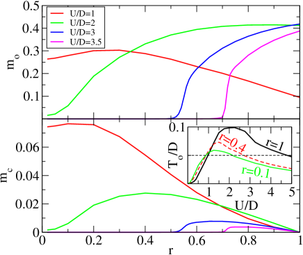
Figure 9: Orbital order parameter (upper panel) and charge density wave order parameter (bottom panel) as a function of $r$ for different values of $U$ and $T/D=0.05$. Inset: $T_{o}$ for different values of $r$ as a function of $U$. The horizontal dashed line corresponds to $T/D=0.05$, which is the temperature used for computing $m_{o}$ and $m_{c}$.

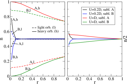
Figure 10: Left panel: Number of light and heavy particles on the A and B sites as a function of $r$ for different values of $U$ and $T/D=0.01$. Right panel: $n_{A}$ and $n_{B}$. Notice that $n_{A}\neq n_{B}$ for $U$=$D$, while for $U$=0.2$D$ the CDW disappears for $r>0.1D$.

All of these results are consistent with the behaviour of the double occupancy, which can actually be experimentaly measured in cold atom systemsStöferle et al. (2006). In Fig. 11, we plot the double occupancy $d=$$\langle n_{h}n_{l}\rangle$ in both sublattices in the ordered phase and also its value in the disordered phase. The fact that true CDW order accompanies the orbital order immediately implies that $d$ can show different behaviours on each of the sublattices. This is indeed the case as shown in Fig. 11, where $d_{A}$ and $d_{B}$ are different within the ordered phase ($T<T_{o}$), when $r\not=1$.

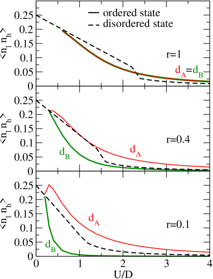
Figure 11: Double occupancy $d_{A}$ and $d_{B}$ (solid lines) for different values of $U$ and $r$ at $T/D=0.01$. For comparison, the dashed lines represent the equivalent curves for the disordered state. The sharp behavior at low $U$ is a signature of the disorder-order transition at finite $T$.

In the symmetric case, $r=1$, we observe that, for moderate to strong interactions, the double occupancy of the ordered phase is higher than in the disordered one. This is due to the fact that in a state with staggered order, hopping to a neighboring site is less penalized by Pauli blocking with respect to the situation in a disordered stateGorelik et al. (2010). On the contrary, for small to moderate coupling the behavior is the inverse, since in the disordered metallic state the particles delocalize on both orbitals, increasing the probability of double occupation. The ordered state remains an insulator even at small $U$, thus favoring orbital localization. At low enough $U$, the ordered state eventually becomes unstable at the finite $T$ of our numerical calculations, ie, when $T>T_{o}(U)$.

For $r\neq 1$, we observe the effects of the onset of the CDW. The behavior of the double occupancy becomes different on each sublattice, as previously discussed. At low couplings, we find that the difference has a sudden increase, which reflects the steep rise of the orbital order-parameter $m_{o}$ as the system enters the ordered phase. This shows that an abrupt change in the sublattice double occupation is a good probe of CDW order in a system. This sharp behaviour reduces with increasing $r$ as expected because the CDW order decreases with increasing $r$, fully disappearing in the limit of $r=1$. We also see that, for any value of $U$, the double occupancy is higher in the HM and decreases with decreasing $r$ which is consistent with the fact that as $r$ decreases it gets harder for the heavier particle to hop from one lattice site to another. These results confirm that asymmetric hopping amplitudes favor a CDW, which can be experimentally detected. Alternatively, this also suggests that the density distribution can be manipulated by tuning the hopping ratio $r$.

III.2.3 Thermodynamics

One of the challenging aspects of cold atomic systems in optical lattices is the determination of their temperature. To this end, it is important to know the thermodynamic properties of the system. With this issue in mind, we focus on the computation of the fundamental thermodynamic quantities: specific heat and entropy of the AHM in this section. We set the Boltzmann constant $k_{B}=1$.

In our previous paper Winograd et al. (2011), we discussed the specific heat $C_{\rm V}$ and the entropy per site (or equivalently per particle if working at $n_{tot}=1$) $S/N$=$s$ in the disordered phase of the AHM. The main features can be summarized as follows (see Fig. 12 where we plot these quantities at a finite generic value of $r$): In the metallic phase at low $U$, the $C_{\rm V}$ and $s$ are linear in $T$, for all values of the asymmetry parameter $r\not=0$ and $T<T_{coh}$. This behavior is a signature of the Fermi liquid groundstate. At $T\approx T_{coh}$, the $C_{\rm V}$ develops a peak and the entropy has a small plateau at $s=\ln(2)$, that corresponds to the two orbital degrees of freedom. In the Kondo impurity problem, this scale indicates the destruction of the Kondo singlet state [$(|lh\rangle-|hl\rangle)\to(|l\rangle\bigotimes|h\rangle)$] . Increasing $T$ further, $s$ increases and eventually saturates at $s=\ln(4)$ at high $T$. This value corresponds to the four different states available per site, ie $|0\rangle,|h\rangle,|l\rangle,|lh\rangle$. On the other hand, $C_{\rm V}$ develops a second peak due to the excitation of states of the incoherent Hubbard bands.

Figure 12: Specific heat and entropy per site as a function of $T$ for $r=0.4$, in the disordered case for $U=D$ (metal) and $U=2D$ (insulator). For reference, $T_{coh}$ is indicated by the vertical dotted line. It corresponds to the destruction of the Kondo effect, the first peak in the $C_{\rm V}$  and the $\ln(2)$ plateau in $S/N$.

The behavior of the entropy in the Mott state of the AHM, shown in Fig. 12, resembles that of the metallic state of the standard FKMWinograd et al. (2011). However, the similarity is superficial, and is due to different physical reasons. In the latter, the heavy particles have zero hopping amplitude and are localized, thus there is an equal probability of finding a heavy particle or not on any given site. Therefore, there are two occupation states associated with any site and this contributes a factor of $\ln(2)$ to the entropy, even as $T\to 0$. As $T$ increases, the entropy increases monotonically to the asymptotic value $\ln(4)$. However, in the Mott insulating state of the AHM, both particle species are localized and, in contrast to the FKM case that we just described, there are two different ways of singly occupying a site ($|h\rangle$ or $|l\rangle$), hence the $\ln(2)$ in the entropy. As before, at high $T$, density fluctuations are thermally activated, hence the entropy and $s$ also goes continuously to $\ln(4)$. Regarding the behavior of the $C_{\rm V}$  since the insulating Mott state of the AHM is characterized by the opening of a correlation gap, the specific heat displays activated behavior at low $T$.

The behavior of the specific heat in the ordered phase shows clear signatures of a phase transition. The results are shown in Figs. 13 and 14 for characteristic values of the parameters $r$ and $U$. At very low $T$, the $C_{\rm V}$ has activated behavior (the internal energy is almost constant), due to the opening of the insulating gap in the orbitally ordered state. Increasing $T$, the system eventually reaches the transition temperature $T=T_{o}$ where the order is lost. The internal energy plotted in Fig. 13 shows a sudden upturn as the state becomes unstable. At the critical point there is a kink which translates to a divergence in the specific heat.

In Fig. 15 we plot the entropy in the ordered state for $r=0.4$ and several values of $U$. The data shows activated behavior at very low $T$ and a rapid increase of the thermal excitations as the temperature approaches $T_{o}$ and the ordered moment melts (see Fig. 7). For $T$ above $T_{o}$, in the disordered phase, the entropy is identical to that of Fig. 12. The non-monotonic behavior of the position of the maxima, is simply a consequence of the peculiar behaviour of $T_{o}$ with $U$ that was already discussed Sec. III.2.1.

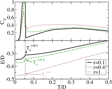
Figure 13: Specific heat and internal energy as function of $T$ for $U=D$, and different values of $r$ in the ordered phase. The first peak in $C_{\rm V}$ reveals a formation of an orbitally ordered phase, while the second, the localization of the particles. The sharp reduction of the internal energy when decreasing $T$, reveals the formation of an insulated-orbitally ordered state, at $T_{o}$. For $U=D$, $T_{o}$ is weakly dependent on $r$, as shown in Fig. 8.

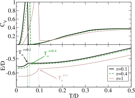
Figure 14: Specific heat and internal energy as function of $T$ for $U=2D$, and different values of $r$ in the ordered phase. Note that for $U=2D$, $T_{o}$ increases with $r$.

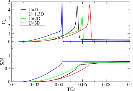
Figure 15: Specific heat and entropy as a function of $T$ for $r=0.4$ and $U/D=1,1.3,2,3$, in the ordered phase. Above $T_{o}(U)$, where the $C_{v}$ has a kink, the entropy coincides with that of the disordered state. For low enough $T$, the activated behavior is non-monotonic in $U$, revealing the different natures of the ordered state with varying $U$.

III.3 Proposal for cooling mechanism: Entropic chromatography

Despite the fact that experiments on cold atoms in optical lattices are done at ultra low temperatures, it is necessary to achieve even lower temperatures, to access new interesting strongly correlated quantum phases.

One of the theoretical schemes proposed for cooling, is based on the idea of embedding a fermionic gas in an optical lattice within a bosonic bath, and then ‘squeezing’ out the entropy of the fermions. This may be achieved by first shrinking their trap, thus compressing the fermionic gas towards a band insulator state. This state has no free degrees of freedom left, hence, no entropy (with the exception of the states at the edges of the trap). The lost fermionic entropy is thus transferred to the bosonic bath, and the bosons are then released. The remaining fermions are in a low entropy state, therefore at a much lower temperature Ho and Zhou (2009). Another proposalBernier et al. (2009), suggested modifications to the shape of the harmonic trap so as to create a deep dimple in the center where one would form a band insulator. This separates the system into an entropy poor state at the center, surrounded by entropy rich regions. The entropy rich particles could subsequently be removed from the system by partially opening the trap and the remnant band insulator could then be adiabatically relaxed to the relevant experimental regime.

Motivated by the present study of the AHM, here, we propose an alternative scheme to cool the system based on the principal feature of the AHM i.e., the hopping asymmetry. In Fig.16, we plot the entropy per site $s$, in the non-interacting limit ($U=0$) limit of the AHM at half filling. We see that most of the entropy is carried by the heavier particles for $T<0.4D$. The difference in entropy between the two species is more pronounced at very low temperatures. Though we have not included the effect of the trapping potential in our calculation, we do not expect it to significatly change the nature and validity of the cooling mechanism that we shall describe.

The ability to concentrate most of the entropy in the heavy species by manipulating the hopping amplitudes of one species, immediately suggests the possibility of an entropic chromatography method. One can repeatedly concentrate entropy in one of the species and use the other as a thermal bath, which is then partially evaporated, liberating entropy (ie heat) at each successive step. This leads to a big reduction of entropy of the remanent system, hence reducing its temperature. Our cooling scheme is based on this entropic chromatography, supplemented with a series of system parameters modifications, to ensure that the physical system stays within the required filling regime (ie one particle per site on average). This scheme is similar to those mentioned above, in that we separate the system into entropy rich and entropy poor sectors, with the main difference being that here the entropic separation is not spatial. The advantage of this procedure is that it does not require an additional Bose condensate to act as a reservoir or additional lasers to modify the trapping potentials in a precise manner. Our scheme essentially relies on the possibility of having two different fermionic atomic species within their respective atomic traps, which can be independently adjusted. We describe our cooling procedure in detail below.

We consider a system where the light and heavy particles have their respective trapping potentials and their interaction is described by the AHM. We limit our analysis to the disordered phase of the AHM. However, the extension of the idea to the long-range ordered phase can be performed along similar lines. In this section, for the sake of clarity in the description of the procedure, we denote the two atomic species as particles of type 1, and type 2. We assume that all the system parameters (hopping, $U$, trapping potential) can be tuned adiabatically and that the system thermalizes to an equilibrium state. The cooling scheme to be described below is useful and applicable provided the initial temperature and entropy of the system is such that in the non-interacting limit, the difference in the entropies of the light and heavy particles is substantial.

We summarize the cooling scheme in the following steps :

1. Start by loading $N_{1}=N_{2}=N$ particles of each fermionic species into the optical lattice at finite $U$ and hoppings

   $$t_{1} = t$$

   $$t_{2} = \alpha t$$ (10)

   with an asymmetry $\alpha\ll 1$. The parameter $\alpha$ actually plays the same role as the ratio $r$, however, we use this convention to emphasize that $\alpha$ is varied during the cooling procedure. The entropy of this initial state is denoted as $S_{tot}^{(i)}$. The trap and the optical lattices are adjusted such that the system is half-filled.

2. The interaction is now adiabatically tuned to $U=0$. Since this is an isentropic process, the entropy of the resulting system is the same as that of the initial state. However, as shown in Fig. 16, in this non-interacting limit, the entropy of the system is now mostly carried by the heavy particles $2$.

   

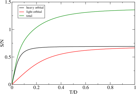
   Figure 16: Entropy per lattice’s site in the non-interacting system for $r=0.2$.

   For non-interacting fermions (or quasiparticles in a Fermi liquid), at low $T$ the entropy is proportional to $T$ Nozières (1997): $S={\kappa_{B}^{2}k_{F}mT}/{3\hbar}$ where the mass of the particles (or the effective mass of the quasiparticles in the Fermi-liquid regime) $m$ is proportional to the inverse of the hopping amplitude $t$ and $\kappa_{B}$ is the Boltzmann’s constant. This implies that at this step of the cooling process, the entropy of the system can be expressed as:

   $$S_{tot}^{(i)} = Ns_{1}^{(1)}+Ns_{2}^{(1)}=\frac{\kappa NT^{(1)}}{t}+\frac{\kappa NT^{(1)}}{\alpha t}$$ (11)

   $$= \kappa N\frac{T^{(1)}}{t}\left(1+\frac{1}{\alpha}\right)$$

   where $s_{j}^{(1)}$ is the entropy per particle of species $j$=1, 2 at this step, and $T^{(1)}$ is the new temperature resulting from the adiabatic variation of $U$. $\kappa$ is some proportionality constant which is the same for both species (cf. Fig.16).

3. Open the trap of particles $2$, and free half of them. The released entropy ($S_{-}^{(1)}$) is:

   $$S_{-}^{(1)}=\frac{\kappa NT^{(1)}}{2\alpha t}$$ (12)

4. Turn on $U$ adiabatically so the particles interact and thermalize (we assume here that the relaxation time is fast). The system now has an unequal number of particles of both species and a total entropy $S_{tot}^{(2)}=S_{tot}^{(i)}-S_{-}^{(1)}$

5. To eliminate the excess number of particles of species 1 and to reduce the entropy further, we adiabatically invert the ratio $t_{2}/t_{1}$, in order to have,

   $$t_{1} = \alpha t$$

   $$t_{2} = t$$ (13)

6. The interaction is again adiabatically tuned to $U=0$. We now have a state with total entropy $S_{tot}^{(2)}$ such that

   $$S_{tot}^{(2)} \equiv Ns_{1}^{(2)}+\frac{N}{2}s_{2}^{(2)}=\frac{\kappa NT^{(2)}}{\alpha t}+\frac{\kappa NT^{(2)}}{2t}$$ (14)

   where $s_{1}^{(2)}$ and $s_{2}^{(2)}$ denote the entropies per particle of the two species and $T^{(2)}$ the resulting temperature at this step.

7. We open the trap for particles $1$, and eliminate $N/2$ particles of type 1. The freed entropy at this step is $S_{-}^{(2)}=\frac{\kappa NT^{(2)}}{2\alpha t}$ and the total residual entropy is

   $$S_{tot}^{(3)}=S_{tot}^{(2)}-S_{-}^{(2)}$$ (15)

8. To obtain the final state with $N/2$ particles of each species and to thermalize the system so as to have a well defined temperature, we, once again, invert the ratio $t_{2}/t_{1}$, at finite $U$. The traps of both species are narrowed, adapting the number of sites ensuring that we have a half-filled system.

9. In order to compare the temperature of this final state with the initial one, we turn off $U$. This final state has equal numbers of particles $N/2$ of each species and the same hopping ratio as in step i and an entropy

   $$S_{tot}^{(f)}=S_{tot}^{(3)}=\frac{\kappa NT^{(f)}}{2t}(1/\alpha+1)$$ (16)

   The isentropic processes also ensure that the temperature of this state $T^{(f)}=T^{(2)}$, which follows from Eqs. (14), (15) and (16). Then, by matching the final entropy of Eq. 16 with

   $$S_{tot}^{(f)}=S_{tot}^{(1)}-S_{-}^{(2)}-S_{-}^{(1)}$$ (17)

   we find that

   $$\frac{T^{(f)}}{T^{(1)}}=\frac{2\alpha+1}{\alpha+2}$$ (18)

Note that the initial temperature of the mixture $T^{(i)}$ is not know, the first temperature that could be defined was $T^{(1)}$ at step (ii) with Eq. 11. From the last expression and Eqs. 11 and 16 it also follows that the ratio of the total final and initial entropies is $S_{tot}^{(f)}/S_{tot}^{(i)}=T^{(f)}/2T^{(1)}$, thus that the entropy per particle in the $U=0$ limit can be reduced by the same factor $T^{(f)}/T^{(1)}$. We also see from (18), that no reduction of entropy or temperature is achieved in the Hubbard limit $\alpha\to 1$ and that the cooling is entirely a consequence of the anisotropy in the hoppings. The maximal reduction $T^{(f)}=T^{(1)}/2$ is obtained in the FK limit, $\alpha\rightarrow 0$. Note that depending on the number of particles loaded into the optical lattice and the final system required, the cooling procedure can be repeated a finite number of times, resulting in a drastic reduction of the temperature.

However, we should mention that in cold atom experiments, currently accessible entropies per particle are of the order of $s\simeq 1.5$. This value is well outside the linear regime discussed here (cf. Fig. 16) and the analytical result obtained here, though helpful to illustrate the mechanism, is quantitatively invalid. Nevertheless, we emphasize that the cooling procedure i-viii, should still qualitatively work within a wider window of $T$, since the large difference in entropy persists well beyond the linear regime (cf. Fig. 16).

Within our approximation, we now attempt to estimate the efficacy of our cooling procedure for the interacting system. In Fig. 17, we plot the entropy of the interacting ($U$=$D$) and the non-interacting system, for $t_{2}/t_{1}$=0.2 at half-filling. In this example with $\alpha$=0.2, we see that starting from $U$=$D$ and entropy per site (at half filling is identical to per particle) $s$=1, the initial temperature is about $T_{int}^{(i)}/D\simeq 0.28$. Then, first by decreasing $U$ to zero, we see that it corresponds to a temperature $T^{(1)}\simeq 0.175D$. Following the steps i-viii, we can use eq. 18 to estimate the temperature of the new state. In this example, the temperature of the non-interacting system would be $T^{(f)}\simeq 0.11D$, which according to Fig. 17, corresponds to an entropy of $s\simeq 0.83$. Then, adiabatically turning on the interactions to $U$=$D$, it would be possible to get an interacting state that corresponds to a temperature of $T_{int}^{(f)}/D\simeq 0.16$, which is about a 40% lower than the initial temperature However, we reiterate that this number is only an estimate, since we have used Eq. 18 which is accurate only in the linear regime. In any case, the percentage could be further increased by increasing the hopping asymmetry, i.e., reducing $\alpha$. The cooling procedure can be repeated a number of times to access even lower entropies and temperatures. It would also be interesting to see how this scheme works if we take into account the trapping potential and also consider ordered initial states. This can be done numerically and is left for future work.

Regarding the actual implementation of the cooling procedure in experimental setups, we would like to point out that our proposal has the simple goal of showing that the hopping asymmetry can potentially be exploited to cool the system once it has been loaded onto an optical lattice. Though the hopping and interaction parameters can in principle be tuned over a wide range, a main experimental concern is how to remove the excess of entropy from the system in a controlled manner. This is a very challenging issue and is the subject of ongoing work. Another important aspect is the equilibration times of the system. These are topics of great experimental relevance and remain beyond the scope of the present study.

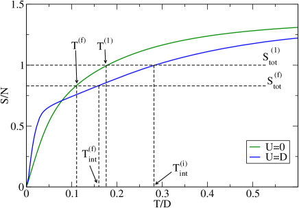
Figure 17: Entropy as a function of $T$ with a hopping asymmetry $t_{2}/t_{1}=0.2$, for $U=0$ and $U=D$. $T^{(1)}$ ($T^{(i)}_{int}$) corresponds to the temperature of the non-interacting (interacting) state, with $S/N=1$, while $T^{(f)}$ ($T_{int}^{(f)}$) correspond to that of the final state (after doing the cooling procedure, and taking $\alpha=0.2$).

III.4 Cooling by tuning hopping and interactions

The success and applicability of the cooling procedure discussed above depends crucially on the changes in temperature induced by the adiabatic variation of the model parameters in the AHM. More precisely, a key issue is whether adiabatic changes of $U$ and $t_{\sigma}$ will heat or cool the systemWerner et al. (2005); De Leo et al. (2011). In this section, we analyze the temperature changes in the AHM as the parameters $U$ and $r$ are varied. As in the previous section, we restrict our study to the disordered phase, but the generalization to a long-range ordered phase is straightforward. From Refs. Werner et al., 2005; De Leo et al., 2011, we know that any change of a parameter $x$ in the Hamiltonian, will result in an entropy change which is linked to a temperature change as follows:

$$-\frac{1}{c}\left.\frac{\delta s}{\delta x}\right|_{T}=\left.\frac{1}{T}\frac{\delta T}{\delta x}\right|_{s}$$ (19)

where $c=T\delta S/\delta T$ is the specific heat ($c$ is always possitive).

Using Maxwell’s relations,

$$\left.\frac{\delta s}{\delta U}\right|_{N,t_{\sigma},T}=-\left.\frac{\delta d}{\delta T}\right|_{N,t_{\sigma},U}$$ (20)

$$\left.\frac{\delta s}{\delta t_{\sigma}}\right|_{N,U,t_{-\sigma},T}=-\frac{1}{t_{\sigma}}\left.\frac{\delta E_{kin,\sigma}}{\delta T}\right|_{N,t_{\sigma},U}$$ (21)

and (19), we obtain the following expressions for the change in temperature for fixed entropy, when the Hamiltonian parameters $U,t_{\sigma}$ are varied,

$$\frac{1}{T}\left.\frac{\delta T}{\delta U}\right|_{S,N,t_{\sigma}}=\frac{1}{c}\left.\frac{\delta d}{\delta T}\right|_{N,t_{\sigma},U}$$ (22)

$$\frac{1}{T}\left.\frac{\delta T}{\delta t_{\sigma}}\right|_{S,N,U}=\frac{1}{ct_{\sigma}}\left.\frac{\delta E_{kin,\sigma}}{\delta T}\right|_{N,t_{\sigma},U}$$ (23)

The changes in temperature when the interaction $U$ is varied is given by the temperature variation of the double occupancy, whereas, the change in temperature induced by the variation of $t_{\sigma}$ is dictated by the derivative of the kinetic energy of the particle species $\sigma$ with respect to the temperature. As explained in Ref. De Leo et al., 2011, Eq. (22) suggests that increasing the interactions will cool (heat) the system whenever the temperature derivative of the double occupancy is negative (positive). In a similar way, Eq. 23 shows that increasing the hopping amplitude will heat (cool) the system if the temperature derivate of the kinetic energy is positive (negative).

We now analyze the consequences of tuning theses parameters in the particular case of half-filling without the trapping potential. In Fig. 18 we plot the double occupancy as a function of $T$ for various values of the interaction $U$ and $r$. As pointed out in Ref. Werner et al., 2005 for the Hubbard model, at weak coupling, increasing $U$ heats up the system if one is at high enough $T$ because $\delta d/\delta T>0$. For $T<T_{m}$, where $T_{m}$ is the temperature at which the double occupancy is the lowest, $\delta d/\delta T<0$ , we have a Pomeranchuk like effect where the system cools with increasing $U$. This cooling effect is lost at strong couplings, where the system is insulating and the double occupancy does not vary at low $T$ and always has positive slope. Consequently, there will be neither cooling nor heating of the system whenever $T$ is small, and there will be heating if $T$ is big enough to fill the gap. We find that all of these features, first predicted for the HM, exist in the AHM case also (cf. top panels of Fig.18).

We now focus on temperature changes induced by the variation of the hoppings. In Fig. 19, the kinetic energy for each species is plotted as a function of $T$. For low $U$, i.e. in the metallic phase, the kinetic energy of both species increases monotonically with $T$ for all $r$. From Eq. 23, this implies that there will always be heating of the system as one increases $t_{\sigma}$ in the entire temperature range of interest. In the insulating regime, since the system is in a Mott state, the kinetic energy remains practically constant at low $T$ for both species (especially, the heavier one). Despite the minor variations seen at higher $T$ we expect that a change of hopping parameters at large $U$ leaves the temperature of the system effectively unchanged. These results bode well for the cooling procedure outlined earlier. It would be very interesting to use the results of this section to calculate the exact change in temperature resulting from finite variation of the Hamiltonian parameters during the cooling cycle. This is left for future work.

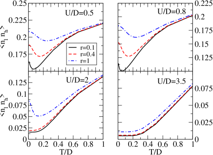
Figure 18: Double occupancy as a function of $T$, for four values of the interaction (one for each panel), and three different values of the ratio $r$.

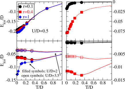
Figure 19: Kinetic energy as a function of $T$ for $l$-particles (left panels) and $h$-particles (right panels). Upper panels: $U/D=0.5$; lower panels: $U/D=2$ (filled symbols) and $U/D=3.5$ (empty symbols); black circles, red squares and blue diamonds corresponds to $r=0.1,0.4,1$, respectevely.

IV Conclusions

In the present work we have studied the AHM as a minimal model to explore multiorbital correlated physics in cold-atoms. We obtained the phase diagram including both ordered and disordered phases. The disordered phase was found to exhibit an interesting orbital selective crossover at finite temperatures to the non-Fermi liquid phase that we first described in Ref. Winograd et al., 2011. We showed that the slope of the momentum dependent density distribution at the Fermi energy may be a convenient observable to probe and characterize this orbital-selective state at finite $T$. In the ordered phase, which was the main focus of the present study, we showed that the AHM displays orbital order coexisiting with a charge density wave whenever $r\not=1$. We computed the behavior of experimentally accesible observables, such as double occupancy, which provided clear signatures of the onset of the ordered state. We also found the regimes of hopping ratio and $U$ where the ordering temperature is highest, that is, where it may be easier to access the ordered phase. We also discussed the relation between orbital order and the onset of charge density waves, which may provide a practical route for manipulating the density distribution inside optical lattices.

Finally, we presented a new strategy to cool fermions in optical lattices using entropic chromatography exploiting the features of entropy concentration that follows from hopping asymmetry. In fact, currently achievable entropies per particle $s\simeq 1.5$ are still too high to even observe the intermediate temperature orbital selective state discussed in this paper, which is characterized by an entropy per particle $s\simeq 0.5-0.8$. This cooling procedure might be a very efficient method to achieve the low temperatures required to access exotic correlated states in cold fermionic systems in optical lattices. An obvious extension of our work would be to include the trapping potential in the AHM. Though this would result in quantitative changes to the the ordering temperatures, entropies per particle in the various phases, etc., we still expect the phase diagram and the physics discussed in this paper to be valid in the bulk of the system. We hope that this work may motivate further experimental developments and provide new bridges between the area of cold atoms and condensed matter physics.

E.A.W. acknowledges support from the French program ANR-09-RPDOC-019-01.

Appendix A Analytical expressions of the observables

For completeness, in this appendix we present the different expressions used to compute the physical observables from the DMFT calculation. The order parameters are linear combinations of the number of particles, and can be easily computed from the Matsubara Green’s functions obtained by solving the DMFT equations. For a given sublattice $\alpha$ and species $\sigma$,

$$n_{\alpha\sigma}=\frac{1}{\beta}\sum_{\omega_{n}=-\infty}^{\infty}G_{\alpha\sigma}(i\omega_{n})\exp(i\omega_{n}0^{+})$$ (24)

Taking into account the problem of convergence involving $|\omega_{n}|\rightarrow\infty$, Eq. 24 can be expressed in the more numerically tractable manner as

$$n_{\alpha\sigma}=\frac{1}{2}+\frac{1}{\beta}\sum_{\omega_{n}=-\infty}^{\infty}\textrm{Re}\left[G_{\alpha\sigma}(i\omega_{n})\right]$$ (25)

The thermodynamical observables, however, require the calculation of the internal energy $E=\langle H\rangle$. In the disordered phase, the kinetic term is given by

$$E_{\textrm{kin},\sigma}=\frac{1}{\beta}\sum_{k,\omega_{n}}(\epsilon_{k\sigma}-\mu)G_{\sigma}(k,i\omega_{n})e^{i\omega_{n}0^{+}}$$ (26)

Within DMFT for the Bethe lattice it can be rewritten as Georges et al. (1996),

$$E_{\textrm{kin},\sigma}=\frac{t_{\sigma}^{2}}{\beta}\sum_{\omega_{n}}\left[G_{\sigma}(i\omega_{n})\right]^{2}e^{i\omega_{n}0^{+}}$$ (27)

For the ordered phase, this expression can be generalized to

$$E_{\textrm{kin},\sigma}=\frac{t_{\sigma}^{2}}{\beta}\sum_{\omega_{n}}G_{A\sigma}(i\omega_{n})G_{B\sigma}(i\omega_{n})e^{i\omega_{n}0^{+}}$$ (28)

The potential energy can be simply computed as $U$ times the double occupancy. In a general case away from half-filling, it might be also necessary to add a term $E_{\mu}=\mu(n_{h}+n_{l})$. The specific heat is then numerically evaluated as

$$C_{v}=\frac{\partial E}{\partial T}$$ (29)

The entropy requires the $T$ integration of the specific heat, since at constant volume $TdS=C_{v}dT$. This can be achieved by integrating $C_{v}/T$ from $T=0$ or $T\rightarrow\infty$. In general, the latter option is better since the asymptotic value $S(T\rightarrow\infty)=N\ln(4)$ is already known, and therefore the expression becomes

$$S(T)=S(\infty)-\int_{T}^{\infty}dT^{\prime}\frac{C_{v}(T^{\prime})}{T^{\prime}}$$ (30)

However, in some cases, such as an ordered state, where there is a singularity in the specific heat, it is also necessary to carry out the integration from $T=0$, which results in

$$S(T)=S(0)+\int_{0}^{T}dT^{\prime}\frac{C_{v}(T^{\prime})}{T^{\prime}}$$ (31)

To use this expression one needs a good justification for the value of $S(0)$.

References

- Hubbard (1963) J. Hubbard, Proc. Roy. Soc. London A276, 238 (1963).
- Georges et al. (1996) A. Georges, G. Kotliar, W. Krauth, and M. J. Rozenberg, Rev. Mod. Phys. 68, 13 (1996).
- Falicov and Kimball (1969) L. M. Falicov and J. C. Kimball, Phys. Rev. Lett. 22, 997 (1969).
- Freericks and Zlatić (2003) J. K. Freericks and V. Zlatić, Rev. Mod. Phys. 75, 1333 (2003).
- Si et al. (1992) Q. Si, G. Kotliar, and A. Georges, Phys. Rev. B 46, 1261 (1992).
- Mandel et al. (2003) O. Mandel, M. Greiner, A. Widera, T. Rom, T. W. Hänsch, and I. Bloch, Phys. Rev. Lett. 91, 010407 (2003).
- Taie et al. (2010) S. Taie, Y. Takasu, S. Sugawa, R. Yamazaki, T. Tsujimoto, R. Murakami, and Y. Takahashi, Phys. Rev. Lett. 105, 190401 (2010).
- Bloch et al. (2008) I. Bloch, J. Dalibard, and W. Zwerger, Rev. Mod. Phys. 80, 885 (2008).
- Cazalilla et al. (2005) M. A. Cazalilla, A. F. Ho, and T. Giamarchi, Phys. Rev. Lett. 95, 226402 (2005).
- Wang et al. (2009) B. Wang, H.-D. Chen, and S. Das Sarma, Phys. Rev. A 79, 051604 (2009).
- Dao et al. (2007) T.-L. Dao, A. Georges, and M. Capone, Phys. Rev. B 76, 104517 (2007).
- Lin et al. (2006) G.-D. Lin, W. Yi, and L.-M. Duan, Phys. Rev. A 74, 031604 (2006).
- Wille et al. (2008) E. Wille, F. M. Spiegelhalder, G. Kerner, D. Naik, A. Trenkwalder, G. Hendl, F. Schreck, R. Grimm, T. G. Tiecke, J. T. M. Walraven, S. J. J. M. F. Kokkelmans, E. Tiesinga, and P. S. Julienne, Phys. Rev. Lett. 100, 053201 (2008).
- Chin et al. (2010) C. Chin, R. Grimm, P. Julienne, and E. Tiesinga, Rev. Mod. Phys. 82, 1225 (2010).
- Nascimbène et al. (2010) S. Nascimbène, N. Navon, K. J. Jiang, F. Chevy, and C. Salomon, Nature 463, 1057 (2010).
- Dao et al. (2012) T.-L. Dao, M. Ferrero, P. S. Cornaglia, and M. Capone, Phys. Rev. A 85, 013606 (2012).
- Alon et al. (2005) O. E. Alon, A. I. Streltsov, and L. S. Cederbaum, Phys. Rev. Lett. 95, 030405 (2005).
- Scarola and Das Sarma (2005) V. W. Scarola and S. Das Sarma, Phys. Rev. Lett. 95, 033003 (2005).
- Isacsson and Girvin (2005) A. Isacsson and S. M. Girvin, Phys. Rev. A 72, 053604 (2005).
- Brydon (2008) P. M. R. Brydon, Phys. Rev. B 77, 045109 (2008).
- Winograd et al. (2011) E. A. Winograd, R. Chitra, and M. J. Rozenberg, Phys. Rev. B 84, 233102 (2011).
- Camjayi et al. (2007) A. Camjayi, M. J. Rozenberg, and R. Chitra, Phys. Rev. B 76, 195108 (2007).
- Gorelik et al. (2010) E. V. Gorelik, I. Titvinidze, W. Hofstetter, M. Snoek, and N. Blümer, Phys. Rev. Lett. 105, 065301 (2010).
- Freericks and Jarrell (1995) J. K. Freericks and M. Jarrell, Phys. Rev. Lett. 74, 186 (1995).
- Freericks (1993) J. K. Freericks, Phys. Rev. B 47, 9263 (1993).
- van Dongen (1991) P. G. J. van Dongen, Phys. Rev. Lett. 67, 757 (1991).
- van Dongen and Vollhardt (1990) P. G. J. van Dongen and D. Vollhardt, Phys. Rev. Lett. 65, 1663 (1990).
- Fáth et al. (1995) G. Fáth, Z. Domański, and R. Lemański, Phys. Rev. B 52, 13910 (1995).
- Stöferle et al. (2006) T. Stöferle, H. Moritz, K. Günter, M. Köhl, and T. Esslinger, Phys. Rev. Lett. 96, 030401 (2006).
- Ho and Zhou (2009) T.-L. Ho and Q. Zhou, Proc. Natl. Acad. Sci. USA 106, 6916 (2009).
- Bernier et al. (2009) J.-S. Bernier, C. Kollath, A. Georges, L. De Leo, F. Gerbier, C. Salomon, and M. Köhl, Phys. Rev. A 79, 061601 (2009).
- Nozières (1997) P. Nozières, Theory of Interacting Fermi systems, edited by Westview Press (Westview Press, 1997).
- Werner et al. (2005) F. Werner, O. Parcollet, A. Georges, and S. R. Hassan, Phys. Rev. Lett. 95, 056401 (2005).
- De Leo et al. (2011) L. De Leo, J.-S. Bernier, C. Kollath, A. Georges, and V. W. Scarola, Phys. Rev. A 83, 023606 (2011).