ROTATION RATES OF THE CORONAL HOLES AND THEIR PROBABLE ANCHORING DEPTHS

Abstract

For the years 2001-2008, we use full-disk, SOHO/EIT 195 $\AA$ calibrated images to determine latitudinal and day to day variations of the rotation rates of coronal holes. We estimate the weighted average of heliographic coordinates such as latitude and longitude from the central meridian on the observed solar disk. For different latitude zones between $40^{o}$ north - $40^{o}$ south, we compute rotation rates, and find that, irrespective of their area, number of days observed on the solar disk and latitudes, coronal holes rotate rigidly. Combined for all the latitude zones, we also find that coronal holes rotate rigidly during their evolution history. In addition, for all latitude zones, coronal holes follow a rigid body rotation law during their first appearance. Interestingly, average first rotation rate ($\sim 438\,nHz$) of the coronal holes, computed from their first appearance on the solar disk, match with rotation rate of the solar interior only below the tachocline.

1 INTRODUCTION

Solar coronal holes (CH) are large regions in the solar corona with low density plasma (Krieger et al. 1973; Neupert & Pizzo, 1974; Nolte et al. 1976; Zirker 1977; Cranmer 2009 and references therein; Wang 2009) and unipolar magnetic field structures (Harvey & Sheeley 1979; Harvey et al. 1982), distinguished as dark features in EUV and X-ray wavelength regimes. During the solar maximum, CH are distributed at all latitudes, while at solar minimum, CH mainly occur near the polar regions (Madjarska & Wiegelmann 2009). In addition to sunspot activity and magnetic activity phenomena that strongly influence the Earth’s climate (Hiremath 2009 and references there in), there is increasing evidence that, on short time scales, occurrences of solar coronal holes trigger responses in the Earth’s upper atmosphere and magnetosphere (Soon et al. 2000; Lei et al. 2008; Shugai et al. 2009; Sojka et al. 2009; Choi et al. 2009; Ram et al. 2010; Krista 2011; Verbanac et al. 2011).

Physics of solar cycle and activity phenomena is not well understood (Hiremath 2010 and references therein). In order to understand the solar cycle and activity phenomena, an understanding of rotational structure of the solar interior and the surface are necessary. On the other hand, rotation rate of the interior and the surface are coupled with the rotation rate of the solar atmosphere, especially the corona. Although there is a general consensus regarding the interior rotation as inferred from the helioseismology (Dalsgaard & Schou 1988; Thompson et al. 1996; Antia et al. 1998; Thompson et al. 2003 and references therein; Howe 2009; Antia & Basu 2010), surface rotation rates as derived from sunspots (Newton & Nunn 1951; Howard et al. 1984; Balthasar et al. 1986; Shivaraman et al. 1993; Javaraiah 2003), Doppler velocity (Howard & Harvey 1970; Ulrich et al. 1988; Snodgrass & Ulrich 1990) and magnetic activity features (Wilcox & Howard 1970; Snodgrass 1983; Komm et al. 1993), there is no such consensus (see also Li et al. 2012) on the magnitude and form of rotation law for features in the corona.

For example, by using coronal holes as tracers (Wagner 1975; Wagner 1976; Timothy & Krieger 1975; Bohlin 1977) and large scale coronal structures (Hansen et al. 1969; Parker et al. 1982; Fisher & Sime 1984; Hoeksema 1984; Wang et al. 1988; Weber et al. 1999; Weber & Sturrock 2002), previous studies show that corona rotates rigidly while other studies (Shelke & Pande 1985; Obridko & Shelting 1989; Navarro-Peralta & Sanchez-Ibarra 1994; Insley et al. 1995) indicate differential rotation. In addition to using coronal holes as tracers, X-ray bright points (Chandra et al. 2010; Kariyappa 2008; Hara 2009), coronal bright points (Karachik et al. 2006; Brajša et al. 2004; Wöhl et al. 2010), and SOHO/LASCO images have been used for the computation of rotation rates and yield a differentially rotating corona. Recent studies using radio images at 17 GHz (Chandra et al. 2009) and synoptic observations of the O VI 1032 $\AA$ spectral line from the SOHO/UVCS telescope (Mancuso & Giordano 2011), however, suggest that the corona rotates rigidly. As part of an ISRO (Indian Space Research Organization) funded project, the present study utilizes SOHO/EIT 195 $\AA$ calibrated images for understanding the following four objectives : (i) to check for latitudinal dependency of rotation rates of the coronal holes, (ii) to study rotation rates of CH during their first appearance on the observed disk, (iii) irrespective of their latitude, to study day to day variation of rotation rates of coronal holes and, (iv) to estimate probable anchoring depths of coronal holes. In section 2, we present the data used and method of analysis, and the results of that analysis in section 3. In section 4, we present the discussion on cause for rigid body rotation rate of the coronal holes and estimate their probable anchoring depths with our conclusions.

2 DATA AND ANALYSIS

For the period 2001 to 2008, we use full-disk SOHO (Solar and Heliospheric Observatory)/EIT images (Delaboudiniére et al. 1995) that have a resolution of 2.6 arc sec. per pixel in a bandpass around 195 $\AA$ to detect coronal holes. The period studied includes both intense activity near solar maximum and the descent of solar activity parameters such as 10.7 cm flux to values of $\sim$ half of their values around that maximum. The obtained images are in FITS format and individual pixels are in units of data number (DN). DN is defined to be output of the instrument electronics which corresponds to the incident photon signal converted into charge within each CCD pixel (Madjarska & Wiegelmann 2009).

We consider coronal holes that appear and disappear between $40^{o}$ north - $40^{o}$ south latitude of the visible solar hemisphere. Using the SolarSoft eit_prep routine (Freeland & Handy 1998), we background subtracted, flat-fielded, degridded and normalized the images. As this calibration involves exposure normalization of the images, now onwards unit of DN is DN/sec. We used the occurrence dates and position of CH from the “spaceweather.com” website. As the “spaceweather.com” is not designed for scientific use, we use readily available occurrence dates of CH only. By using approximate position (heliographic coordinates) of CH from this website, we separate a region from the SOHO/EIT images for further analysis and extraction of relevant physical parameters as described below. CH is also confirmed if it has a bimodal distribution in the intensity histogram.

In order to extract physical parameters of CH from the EIT images, we use FV interactive FITS file editor (http://heasarc.gsfc.nasa.gov/docs/software/ftools/fv/). Depending upon shape of the CH, from the FV editor, a circle or an ellipse is drawn covering the whole region of CH and, average DN (intensity) (that is set as a threshold for detecting the boundary) of CH is computed for detecting the boundary (private communications with Prof. Aschwanden). Similar to Karachik & Pevtsov (2011), for some of the coronal holes, threshold is modified to match the visually estimated boundary. This method yields results consistent with the previous intensity histogram methods (Krista & Gallagher 2009; Krista 2011; de Toma 2011 and references there in). After determining the boundary of CH, we employed SolarSoft coordinate routines to compute the central meridian distance ($l_{i}$) (heliographic longitude from the central meridian) and latitude ($\theta_{i}$) of individual pixels within the CH.

Fig 1(a) shows a full disk, solar image with a typical CH close to the center and in the north-east quadrant, while Fig 1 (b) represents the same CH with its threshold DN contour map. In Fig 2(a), DN histogram of the CH is presented. The bimodal distribution in the histogram confirms the DN values in the CH region (Krista & Gallagher 2009; Krista 2011). We summed the total number of pixels and total DN within the CH boundary, which in turn allowed us to compute average heliographic coordinates such as latitude ($\theta$) and central meridian distance (L) of CH as follows:

$$\theta=\frac{\displaystyle\sum\limits_{i=1}^{n}\theta_{i}*DN_{i}}{\displaystyle\sum\limits_{i=1}^{n}DN_{i}}\,\,\,\,\,\,\,\,\,L=\frac{\displaystyle\sum\limits_{i=1}^{n}l_{i}*DN_{i}}{\displaystyle\sum\limits_{i=1}^{n}DN_{i}}\,,$$ (1)

where $\theta_{i}$, $l_{i}$, and $DN_{i}$ (for $i=1,n$, $n$ is number of pixels) are the latitude, the central meridian distance, and DN values of individual pixels. This method of finding the average heliographic coordinates of CH is equivalent to a method in physics of finding the center of mass of an arbitrary geometrical shape.

Table 1: Computation of heliographic coordinates with different weights in equation 1.

CH1			CH2		CH3
Weights	Longitude	Latitude	Longitude	Latitude	Longitude	Latitude
	(Degree)	(Degree)	(Degree)	(Degree)	(Degree)	(Degree)
DN	-8.374	12.604	8.352	-11.727	4.011	-3.898
1/DN	-8.445	12.836	8.637	-12.682	3.818	-3.996
Average	-8.400	12.715	8.489	-12.206	3.917	-3.945

As the average heliographic coordinates of CH are weighted by the intensity (DN counts) of the relevant pixel, thus one can argue that more weight is given to brighter pixels. However, this argument can not be valid as the intensity is weighted in the denominator also (see above equation 1) and, hence, whatever higher weights given to the brighter pixels in the numerator are also equally compensated by the higher weights in the denominator. We also checked with another weighting that emphasizes areas darker than the image mean, $(i.e.,(\sum\limits_{i=1}^{n}DN_{i}/N)-DN_{i}))$ and obtained the same results of average heliographic coordinates suggesting that weighted average used in equation (1) is correct and is not biased towards the brighter pixels.

For computation of heliographic coordinates of CH, we also used weights with inverse of DN (1/DN) and without weights (i.e., simple averages) in equation 1 and the results for three typical CH are presented in Table 1. Negative sign for the longitude indicates the CH that are on the eastern side of the central meridian and negative sign for the latitudes indicates the CH that are in the southern hemisphere. One can notice from this table that irrespective of weighted and non-weighted averaging, computed heliographic coordinates of CH are nearly same.

Fig 1(a)                                                     Fig 1(b)

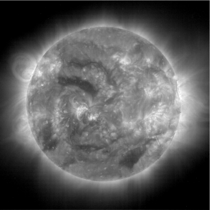
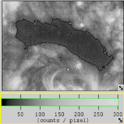
Figure 1: Left side Fig 1 (a) shows full-disk SOHO/EIT 195 $\AA$ image of 01-01-2001, 00:24:11 UT with CH (in the north eastern hemisphere and close to center) and Fig 1(b) illustrates threshold DN contour map of the same CH.

Fig 2(a)                                                     Fig 2(b)

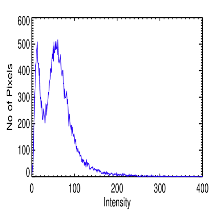
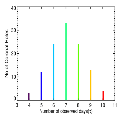
Figure 2: The figure on left side (Fig 2(a)) illustrates DN histogram of a typical coronal hole. Whereas right figure (Fig 2(b)) illustrates total number of CH for number of days ($\tau$) observed on the solar disk.

Following the previous method (Hiremath 2002) of computation of rotation rates of sunspots, daily siderial rotation rates $\Omega_{j}$ of the CH are computed as follows

$$\Omega_{j}=\frac{(L_{j+1}-L_{j})}{(t_{j+1}-t_{j})}+\delta\Omega\,,$$ (2)

where L_j, L_j+1 are average longitudes of the CH for the two consecutive days t_j and t_j+1 respectively, $j=1,2,..n-1$, $n$ is number of days of appearance of CH on the visible solar disk and, $\delta\Omega$ is a correction factor for the orbital motion of the Earth around the Sun. Strictly speaking, this correction factor is due to orbital motion of the SOHO spacecraft around the sun. Compared to the distance between the sun and earth, the distance between the SOHO satellite and the earth is very small and hence orbital distances of earth and the satellite are almost same and hence the correction factor $\delta\Omega$ is $\sim$ 1 deg/day. For the present work, this approximation is sufficient. However, if one wants to find the long term ($\sim$ 11 yrs) variation of rotation rates, correction factor $\delta\Omega$ should be computed accurately (Roša et.al. 1995; Wittmann 1996; Brajša et al. 2002). From the first and second day appearances of CH, one can compute the rotation rate $\Omega_{1}$ that we call as first rotation rate. Similarly for other successive days, rotation rates $\Omega_{2}$, $\Omega_{3}$, etc., are computed. For each computed rotation rate of CH, the respective latitude is assigned as the average of two latitudes corresponding to the two longitudes. We also compute standard deviation and error bars of the average heliographic coordinates and rotation rates. Here onwards computation of rotation rates of CH from equation (2) is called as First Method.

3 RESULTS

Fig 3(a)                                                     Fig 3(b)

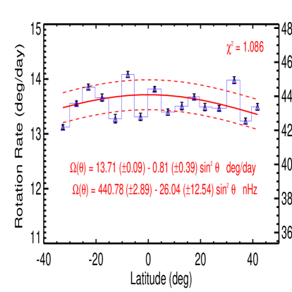
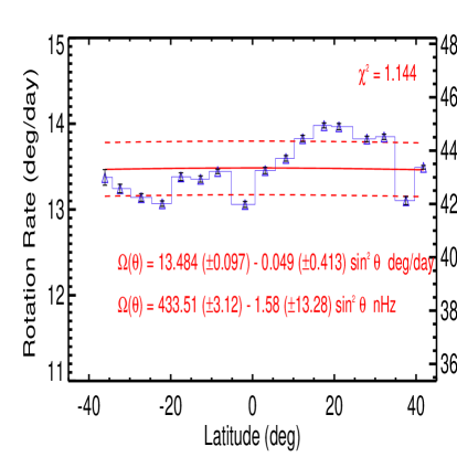
Figure 3: For different latitudes, rotation rates of coronal holes computed from the first method (see section 2). Fig 3(a) for the rotation rates of coronal holes that occur between 65 degrees east and west of the central meridian distance and Fig 3(b) illustrates the rotation rates of CH that occur between 45 degrees east and west of the central meridian distance. In both the figures blue bar plot represents the observed rotation rates; red dashed lines represent the one standard deviation (that is computed from all the data points) error bands and, the red continuous line represents a least-square fit of the form $\Omega(\theta)=\Omega_{0}+\Omega_{d}sin^{2}\theta$ to the observed values. $\Omega(\theta)$ is the observed CH rotation rate, $\theta$ is the latitude, and $\Omega_{0}$ and $\Omega_{d}$ are the constant coefficients determined from the least square fit. $\chi^{2}$ is a measure of goodness of fit.

Fig 4(a)                                                     Fig 4(b)

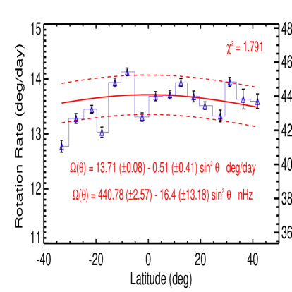
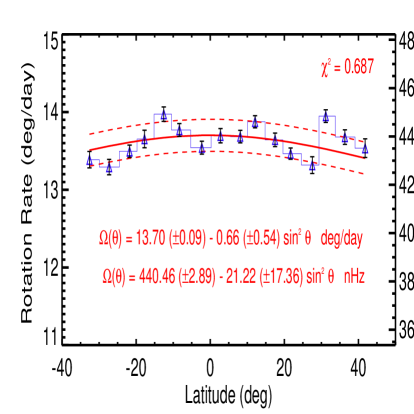
Figure 4: For different latitudes, rotation rates of coronal holes computed from the second method (see section 3.1). Fig 4(a) illustrates the rotation rates of coronal holes that occur between 65 degrees east and west of the central meridian distance and, Fig 4(b) illustrates the rotation rates of CH that occur between 45 degrees east and west of the central meridian distance. In both the figures blue bar plot represents the observed rotation rates; red dashed lines represent one standard deviation (that is computed from all the data points) error bands and, the red continuous line represents a least-square fit of the form $\Omega(\theta)=\Omega_{0}+\Omega_{d}sin^{2}\theta$ to the observed values. $\Omega(\theta)$ is the observed CH rotation rate, $\theta$ is the latitude, and $\Omega_{0}$ and $\Omega_{d}$ are the constant coefficients determined from the least square fit. $\chi^{2}$ is a measure of goodness of fit.

We followed the following criteria in selecting CH data: (i) In order to avoid projection effects (especially coronal holes near both the eastern and the western limbs), we considered only the coronal holes that emerge within 65^∘ central meridian distance, (ii) the coronal hole must be compact, independent, not elongated in latitude, and, (iii) during its passage across the solar disk it should not merge with other coronal holes. For the period of observations from 2001 to 2008, a total of 113 CH satisfy these criteria. We define the term $\tau$ of a CH as total number of days observed on same part of the solar disk satisfying the afore mentioned criteria. Suppose we assume that CH decay due to magnetic diffusion only, as the dimension $L$ of CH is very large (from the following section 3.1, one can note that area $A$ is $\sim 10^{20}cm^{2}$), magnetic diffusion time scale $\tau$ (${L^{2}\over\eta}$ $\sim$ ${A\over\pi\eta}$, where $\eta$ is magnetic diffusivity and area $A$ of CH is assumed to be a circle; magnetic diffusivity in the corona is considered to be $\sim$ $10^{13}cm^{2}sec^{-1}$ (Krista 2011; Krista et.al 2011)) is estimated to be $\sim$ 2 months. Hence, there is a possibility that CH might have reappeared again on the visible disk and might have diffused in the solar atmosphere. Hence, actual life span of CH must be of longer duration. In Fig 2(b), for different $\tau$, we present occurrence number of CH considered for this study.

During their evolutionary passage over the solar disk, we compute rotation rates and assign respective latitudes. If the CH exists for $n$ days, then its $\tau$ is $n$ days and, total number of rotation rates is $(n-1)$. Rotation rates of non-recurrent CH that appear and disappear on the visible disk are computed. According to above definition, and in the present data set (see Fig 2(b)), we find 4 CH that appear for 10 days, 13 CH for 9 days and so on. Integrated over all latitudes and in both the hemispheres, we determined a total of 683 rotation rates.

3.1 Average Rotation Rates : Variations With Respect to Latitude and Area

During their passage over the solar visible disk, daily rotation rates of CH are computed. In both the hemispheres, for each latitude bin of 5^∘, we collect rotation rates and compute average rotation rates with their respective standard deviations $\sigma$ and the errors (${\sigma\over\sqrt{N}}$, where N is number of rotation rates). We present the results in Fig 3 (a) that illustrate the variation of average rotation rates of the coronal holes for different latitudes. To be on the safer side from the projectional effects, we also compute average rotation rates of coronal holes that emerge within 45^∘ central meridian distances and are illustrated in Fig 3(b). For the sake of comparison with helioseismic inferred rotation rates, in both the plots, we include a frequency scale on the right hand side of the vertical axis. For different latitude bins, observed rotation rates are subjected to a least square fit of the form $\Omega(\theta)=\Omega_{0}+\Omega_{d}sin^{2}\theta$ (where $\theta$ is latitude, $\Omega_{0}$ & $\Omega_{d}$ are constant coefficients to be determined).

There is every possibility that as the errors in determination of centers of CH propagate to the rotation rates and hence rotation rates determined from the first method effectively enhance the error in the second coefficient ($\Omega_{d}$) yielding rigid body rotation rates of CH. Moreover, drawback of the first method is also reflected in Fig 3(b) where unlikely asymmetrical rotation profile in both the hemisphere is obtained. In order to minimize such propagating errors in the rotation rates of CH determined by the first method, we compute rotation rates of CH in the following way and define as a Second Method. In this method, as suggested by the referee, we fit all the daily centroid positions of the individual coronal holes by a first degree polynomial and, computed second coefficient (slope) represents the rotation rate. For each computed rotation rate of CH, the respective latitude is assigned by averaging all the latitudes of CH during its passage. As described in the previous paragraph we binned the rotation rates, computed the average rotation rates, standard deviations and error bars respectively. For different latitude bins, average rotation rates are subjected to a linear least square fit and the results are presented in Fig 4. From both the rotation laws, compared to the first coefficient, magnitude of small second coefficient ($\Omega_{d}=-0.81(\pm 1.58)$ in Fig 3(a) or $\Omega_{d}=-0.51(\pm 1.64)$ in Fig 4(a)) suggests that CH rotate rigidly.

Fig 5(a)                                                     Fig 5(b)

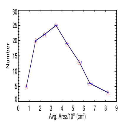
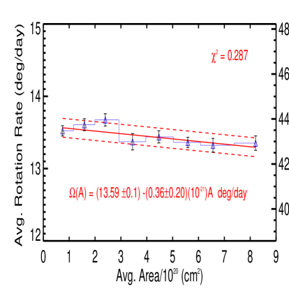
Figure 5: Irrespective of their latitude and number of days ($\tau$) observed on the disk, for different area bins, left figure (5(a)) illustrates occurrence number of CH considered for the analysis and right figure (5(b)) illustrates variation of rotation rates for different average areas. In Fig 5(b), the blue bar plot represents computed rotation rates and the red continuous line represents a least-square fit $Y=a+bX$ to the observed values. $Y$ is observed rotation rate of CH, $X$ is the average area, and $a$ and $b$ are the constant coefficients determined from the least square fit. Red dashed lines in Fig 5(b) represent one standard deviation (that is computed from all the data points) error bands. $\chi^{2}$ is a measure of goodness of fit.

Fig 6(a)                                                     Fig 6(b)

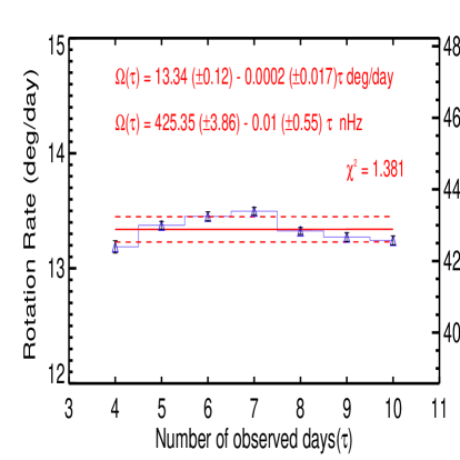
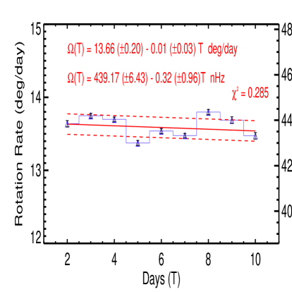
Figure 6: Irrespective of their area and latitude, left (6(a)) and right (6(b)) figures illustrate the variation of rotation rates of CH for different $\tau$ and for different days during their evolution respectively. In both the figures, blue bar plot represents the computed rotation rates and red continuous line represents a least-square fit $Y=a+bX$ to the observed values. $Y$ is the observed rotation rate of CH, $X$ is either $\tau$ or different days represented by $T$, and $a$ and $b$ are the constant coefficients determined from the least square fit. Red dashed lines represent one standard deviation (that is computed from all the data points) error bands. $\chi^{2}$ is a measure of goodness of fit.

Fig 7(a)                                                     Fig 7(b)

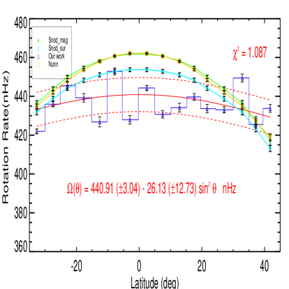
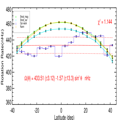
Figure 7: Irrespective of their areas, for different latitudes, blue bar plots that are connected by triangles in both the plots represent the rotation rates of coronal holes as determined from the first method (see section 2). Blue bar plots in both the illustrations represent rotation rates of CH that occur between East and West of 65 (Fig 7(a)) and 45 (Fig 7(b)) degrees central meridian distances respectively. Rotation rates of sunspots (yellow curve; Newton and Nunn 1951), magnetic activity (green curve; Snodgrass 1983) and surface rotation (cyan curve; Snodgrass 1992) are also over plotted. Red dashed lines in both the figures represent one standard deviation (that is computed from all the data points) error bands. $\chi^{2}$ is a measure of goodness of fit.

Fig 8(a)                                                     Fig 8(b)

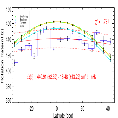
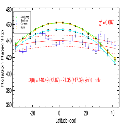
Figure 8: Irrespective of their areas, for different latitudes, blue bar plots that are connected by triangles in both the plots represent the rotation rates of coronal holes as determined from the second method (see section 3.1). Blue bar plots in both the illustrations represent rotation rates of CH that occur between East and West of 65 (Fig 8(a)) and 45 (Fig 8(b)) degrees central meridian distances respectively. Rotation rates of sunspots (yellow curve; Newton and Nunn 1951), magnetic activity (green curve; Snodgrass 1983) and surface rotation (cyan curve; Snodgrass 1992) are also over plotted. Red dashed lines in both the figures represent one standard deviation (that is computed from all the data points) error bands. $\chi^{2}$ is a measure of goodness of fit.

As sunspots show different rotation rates for the small and big areas (Hiremath 2002), it is interesting to know whether similar variations in rotation rates exist in case of coronal holes. As CH evolve, their area also changes and question arises: for which area during the evolutionary passage, rotation rate has to be considered. For this purpose, we adopt the following method. Daily areas and rotation rates of CH are computed. For all the days of CH${}^{{}^{\prime}}$ existence, average area and rotation rates are computed. Further, irrespective of their latitude and $\tau$, rotation rates are collected for the area bins (0-1)$\times 10^{20}cm^{2}$, (1-2)$\times 10^{20}cm^{2}$, etc, and mean rotation rates are computed. In Fig 5(a), we present occurrence number of CH for different area bins. Whereas, irrespective of their latitudes and $\tau$, for different area bins, Fig 5(b) illustrates the mean rotation rates of CH. It is important to note from Fig 5(b) that, unlike sunspots, for different areas, all the coronal holes (as the second coefficient is almost zero, i.e., $(0.36\pm 0.20)\times 10^{-21}$) rotate rigidly. This important result implies that all the CH must originate from same region of the solar interior that rotate rigidly.

3.2 Average Rotation Rates : Variations With Respect to $\tau$ and Daily Evolution

In order to check dependency of rotation rates of CH with respect to number of observed days $\tau$, daily rotation rates are computed during their evolution. As described in section 3, if CH has $\tau$ of $n$ days, we have $(n-1)$ rotation rates. Irrespective of their areas and the latitude, for each $\tau$, rotation rates are collected and average rotation rate is computed and the results are illustrated in Fig 6(a). We find that, rotation rates of CH are independent of $\tau$.

Further, irrespective of their area and $\tau$, we combined daily rotation rates for all the latitudinal bins; we present the resulting daily average rotation rates in Fig 6(b). If coronal holes rotate rigidly and are independent of latitude, then the integrated rotation rates for all the latitudes should remain constant. For example, let us consider the rotation law (red continuous line) over plotted on Fig 6(b). From this law, when one computes the difference between rotation rates of the first day and the 10th day, the difference is found to be $\sim$ 0.1 degree/day, approximately same magnitude as the formal uncertainty in the value for each bin, once again strongly suggesting that, for all the days during their evolutionary passage, coronal holes rotate rigidly.

Table 2: Sidereal rotation rates (deg/day) obtained by the present and previous studies.

Different	Observations	Wavelength	Coefficients		$|\Omega_{d}$/$\Omega_{0}|$	$\chi^{2}$
regions		region	$\Omega_{0}$	$\Omega_{d}$
Corona	Coronal holes1	EUV	13.71	-0.81	0.059	1.086
Corona	Coronal holes1a	EUV	13.48	-0.05	0.004	1.144
Corona	Coronal holes2	EUV	13.71	-0.51	0.037	1.791
Corona	Coronal holes2a	EUV	13.70	-0.66	0.048	0.686
Corona	Coronal holes3	EUV	13.61	-0.15	0.011	0.202
Photosphere	Doppler Shift4	Visible	14.11	-1.70	0.121
Photosphere	Surface magnetic5	Visible	14.37	-2.30	0.160
Photosphere	Sunspots6	Visible	14.38	-2.96	0.206
Photosphere	Sunspots7	Visible	14.37	-2.59	0.180
Radiative Core	Helioseismic8		13.63	-0.64	0.047	5.401

¹Average rotation rates from the First Method and for the CMD (+65^∘ to -65^∘)

${}^{1}a$Average rotation rates from the First Method and for the CMD (+45^∘ to -45^∘)

²Average rotation rates from the Second Method and for the CMD (+65^∘ to -65^∘)

${}^{2}a$Average rotation rates from the Second Method and for the CMD (+45^∘ to -45^∘)

³First rotation rates for the CMD (+45^∘ to -45^∘)

⁴Snodgrass (1992); ⁵Snodgrass (1983); ⁶Newton & Nunn (1951);

⁷Brajša et.al. 2002; ⁸Antia and Basu (2010)

*CMD-Central Meridian Distance

3.3 Comparison of Rotation Rates of CH With Other Activity Indices

Compared to rotation rates obtained by other surface activity indices (Figures 7 and 8), (i) coronal holes rotate almost like a rigid body and, (ii) on average, coronal holes rotate slower ($\sim$ 440 nHz) than the rotation rates of other activity indices over the latitude range $-40$ to $+40$. The ratio $R=|{\Omega_{d}\over\Omega_{0}}|$ of the two coefficients of each rotational law gives a sense of whether the rotation is rigid or differential. For example, if one computes this ratio for sunspots ($R_{sunspot}$) and for coronal holes ($R_{coronal\_hole}$), it is clear that $R_{sunspot}$ $\gg$ $R_{coronal\_hole}$, as can also be seen from the fifth column of Table 2. In this table, goodness of fit $\chi^{2}$ is also given in the last column. Small value of $\chi^{2}$ (typically $\chi^{2}$ should be $\leq$ (N-n), where $N$ is total number of data points and $n$ is degrees of freedom, in this case $n=2$) implies fit is very good. At least compared with any features lower in the solar atmosphere, it is clear that CH rotate rigidly.

Fig 9(a)                                                     Fig 9(b)

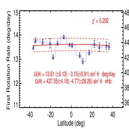
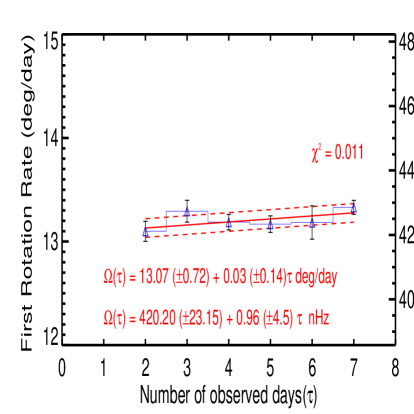
Figure 9: Irrespective of their area and number of days ($\tau$) observed on the disk, left figure (9a) illustrates the variation of first rotation rates of CH with respect to latitude. Irrespective of their area and latitude, for different $\tau$, right figure (9b) illustrates the variation of first rotation rates of CH. Red dashed lines in both the figures represent one standard deviation (that is computed from all the data points) error bands. $\chi^{2}$ is a measure of goodness of fit.

3.4 First Rotation Rates : Variations With Respect to Latitude and Number of Observed Days $\tau$

In the previous subsections, on the basis of small magnitude of second coefficient (as illustrated in Figures 3 and 4) in the rotation law and the ratio $R$ of CH, we concluded that CH rotate rigidly. Although second coefficient is small, it is not completely negligible to conclude unambiguously that CH rotate rigidly. That means a small contribution to the second coefficient due to differential rotation can not be ruled out. This result can be interpreted as follows. The rotation rates of CH presented in the previous sections are combination of rotation rates of CH that are anchored at different parts of the interior during their evolutionary passage on the visible disk. That means if CH are originated only in the convective envelope and raised their anchoring feet towards the surface, owing to differentially rotating convection zone and similar to magnitudes of rotation rates of sunspots, one should get a reliable and large magnitude of second coefficient in the rotation law. On the other hand, if the CH are originated in the radiative core and raised their anchoring feet towards surface, during their first appearance on the surface, one should get combined contribution (from the differential and rigidly rotating regions) to the second coefficient. That means if one computes the first rotation rates $\Omega_{1}$ of CH during their first appearance on the surface for different latitudes and number of days ($\tau$) observed on the disk, one should get unambiguously negligible contribution from the second coefficient of the rotation law. In order to test this conjecture, first rotation rates $\Omega_{1}$ of CH are computed as follows. Again, we consider CH that are born between +65^∘ to -65^∘ from the central meridian. From the first and second day computed longitudes (from the central meridian) of CH and by using first method, first rotation rates are computed. Each first rotation rate is collected in 5^∘ latitude bins and average of the first rotation rates is computed and, for different latitudes, are illustrated in Fig 9(a). Similarly, for different $\tau$, first rotation rates are collected and average of first rotation rates is computed and the results are presented in Fig 9(b). It is important to note that, according to our conjecture, we find that magnitude of the second coefficient has a negligible contribution to the rotation law that leads to inevitable conclusion that CH must rotate rigidly.

From all these results, finally we conclude unambiguously that, independent of their area, number of observed days ($\tau$) and latitude, CH rotate rigidly during the evolutionary passage on the solar disk. However, it is interesting to note from the present and previous studies (Wagner 1975; Wagner 1976; Timothy & Krieger 1975; Bohlin 1977) that although whole coronal hole structure rotates rigidly, individual coronal bright points (CBP) that are embedded in the coronal holes rotate differentially (Karachik et.al. 2006). As pointed by these authors, coronal bright points in the corona might be influenced by the surrounding differentially rotating plasma. However, it is not clear how CBP are influenced by the differential rotation of the surrounding plasma.

4 DISCUSSION AND CONCLUSIONS

In contrast to other persistent solar features of the corona, then, why do coronal holes rotate rigidly? Many observations (Madjarska et.al 2004; Subramanian et.al 2010; Tian et.al. 2011; Yang et.al 2011; Krista 2011; Krista et.al 2011; Crooker & Owens 2011; Madjarska et.al 2012) suggest magnetic reconnection at the coronal hole boundaries (CHBs) as the cause of rigid body rotation.

Pevtsov & Abramenko (2010) conclude that coronal holes^′ rotation rate is almost like rotation rate of sunspots and the CH are “analogous to a grass fire, which supports itself by continuously propagating from one patch of dry grass to the other”. That means coronal hole constantly changes its footprint moving from one available polarity to the other. This implies that area of coronal hole will depends on size of available polarity footprint, and it can either decrease or increase depending on size of photospheric magnetic field patch. This also suggests that, on average, difference in the coordinates at the eastern and western boundaries should remain constant yielding a rigid body rotation rate (as suggested by the previous studies). Thus one can argue that coronal holes are surface phenomena. If the coronal hole is a surface phenomenon and if it constantly changes its footprint moving from one available polarity to other, area of coronal hole depends on size of available polarity footprint. Hence, area should either decreases or increases with a result that, on average, area with respect to time must be nearly constant. In order to test this conjecture, in Fig 10, we illustrate measured areas (that are corrected for projection) of CH that have $\tau$ of 4 days and 5 days (upper panel) and, 6 days and 10 days (lower panel) respectively. Dates of occurrence of these individual coronal holes that are presented in the upper panel of are : 6th Nov to 9th Nov 2001 (2^∘ to 41^∘ East of central meridian); 8th May to 12th May 2004 ( 30^∘ East to 12^∘ west of central meridian) and, dates of occurrence of coronal holes that are presented in the lower panel are: 21st Aug to 26th Aug 2003 (45^∘ East to 11^∘ west of central meridian); 22nd Dec to 31st Dec 2005 (50^∘ East to 62 ^∘ west of central meridian) respectively.

One can notice from Fig 10 that, contrary to expectation (that area of coronal hole nearly remains constant during its evolution), on average, coronal holes^′ area smoothly decrease (upper panel) continuously or increase like sunspots^′ area evolutionary curve, reaches maximum area and then smoothly decreases (lower panel). From these figures, we can not find other expected signatures for the reconnection, viz., substantial daily variations of areas of CH during their evolution. This does not mean that there is no magnetic reconnection at the boundaries. However, in the following, we show that magnetic reconnection alone can not be sufficient for explanation of dynamics (rigid body rotation) and area evolution of the coronal holes. Hence, coronal holes must be deep rooted rather than mere surface phenomena. Interestingly, similar to Bohlin’s (1977) study, we also find the same order ($\sim 10^{14}cm^{2}/sec$) of average growth (or decay) of CH.

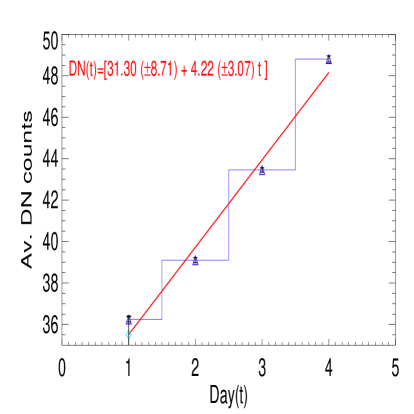
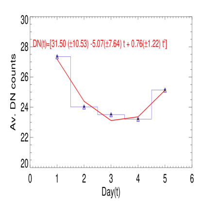
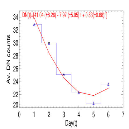
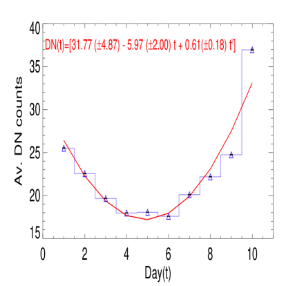
Figure 12: For different days, measured average DN counts of the CH (blue bar plot). Figures in the upper panel are the variation of average DN counts of CH for number of observed 4 and 5 days ($\tau$) respectively. Whereas the figures in the lower panel illustrate variation of average DN counts of CH for number of observed 6 and 10 days ($\tau$) respectively.

One would also expect, magnetic reconnection at the boundary of CH might have a substantial contribution for the enhancement of the average intensity (DN counts). In order to check this expectation, for the same CH presented in Fig 10, we compute the daily average DN counts ($=\frac{\sum\limits_{i=1}^{n}DN_{i}}{N}$, where N is total number of pixels) and are illustrated in Fig 12. Obvious fact from Fig 10 and 12 is that as the area of CH increases, average DN counts (intensity) decrease and vice versa. However, according to our expectation, coronal holes do not show any transient and substantial increase in the intensity during their daily evolutionary passage on the solar disk.

Off course, as CH is embedded in the atmosphere where closed field lines due to active regions coexist and hence, it is natural to expect reconnection at the boundary of a CH due to oppositely directed field lines. Possible reason for the null detection of magnetic reconnection from our data set is due to low temporal resolution of daily data used in this analysis. In fact, with a high temporal resolution of CH data set, majority of previous studies (Wang et al. 1998; Madjarska et al. 2004; Raju et.al 2005; Aiouaz 2008; Madjarska & Wiegelmann 2009; Subramanian et al. 2010; Edmondson et.al. 2010; Krista 2011; Yang et.al. 2011; Madjarska et.al 2012) show the evidences of reconnection, although other studies have lack of such a evidence (Kahler & Hudson 2002; Kahler et al. 2010). If we go by the majority of results that rigid rotation rates of the coronal holes is due to magnetic reconnection at the coronal hole boundaries, then one would expect that the shape (area) of the coronal hole during their disk passage must remains constant. As most of these majority of studies used short ($\sim$ hours) duration data set, question arises whether CH maintain their shape (and hence their areas) through out disk passage (as one can see from our analysis, most of CH exist more than 5 days on the solar disk). One can notice from the area-time plots (Fig 10), during ( $\sim$ days) its disk passage, CH do not maintain their shape and hence rigid body rotation rate of CH is not due to interchange reconnection. As the previous studies use high temporal, short duration ($\sim$ hours) data set and during such time scales (as the CH has a large dimension) obviously one gets constant shape and hence conclusion (that rigid rotation rates of CH is due to magnetic reconnection) is right. However, again we stress from the results presented in Fig 10 that, on long duration ($>$ 5 days), CH do not maintain their shape and rigid body rotation rate of CH is not due to magnetic reconnection alone at their boundaries. Rigid body rotation rate of CH is likely due to their deep rooted anchoring of their feet and subsequently raising towards the surface and then to the atmosphere.

As for area evolution of the coronal hole, question arises as to which is the dominant physical process that dictates temporal variation of area and hence removal of magnetic flux of the coronal hole? Is it due to magnetic diffusion (whose diffusion time scale is $\sim$ ${L\over\eta^{2}}$) or magnetic reconnection at the coronal hole boundaries? Similar to sunspots${}^{{}^{\prime}}$ area evolution curve (Hiremath 2010), formation and growth part of area evolution of CH are not understood. However, in order to answer afore mentioned queries, we consider decay part of the area evolution curve with following two physical reasonings: (i) if area evolution of CH is dominated by magnetic diffusion, then its area must varies as $\sim$ $t^{-1/2}$ (where $t$ is time variable) and, (ii) if area evolution of CH is mainly due to magnetic reconnection, annihilation of magnetic flux due to reconnection of opposite magnetic field lines at the boundaries of the coronal hole leads to an exponential decrease of area with time. If coronal hole is considered to be cylindrical magnetic flux tube with uniform magnetic field structure, from magnetic induction equation (with diffusive dominated term), it is instructive to show that equation for rate of change of magnetic flux $\phi$ is $\frac{d\phi}{dt}=\eta\frac{d^{2}\phi}{dz^{2}}$ (where $\phi$=$\int^{r}_{0}B_{z}Adr$ is magnetic flux of coronal hole flux tube, $A(=2\pi r^{2})$ is area, $t$ is time variable, $\eta$ is magnetic diffusivity, $B_{z}$ is a uniform magnetic field structure along the $z$ direction and $r$ is radius of flux tube). From the results (Krista and Gallagher 2009; CHARM algorithm from solarmonitor.org) illustrated in Fig 11a, absolute magnitude of $B_{z}$ of 10 days CH (during decay part of its area evolution as presented in Fig 10) is found to be nearly independent of time (number of observed days). Using this observational information and assumption that magnetic field structure of coronal hole is also uniform spatially along $r$ direction, it can be easily shown from the rate of change of magnetic flux equation that $\frac{dA}{dt}=\eta\frac{d^{2}A}{dz^{2}}$ and whose solution is obtained as $A\sim t^{-1/2}$ on diffusion time scales.

In order to test these afore mentioned two reasonings, for example, decay part of 10 days area evolution curve is subjected to diffusion and exponential fits. After linearizing the two laws, least-square fits are performed and the result is illustrated in Fig 11b. Compared to exponential fit, for the decay part of area evolution curve, least-square fit for law of diffusion yields very low value of $\chi^{2}$ with the expected decay index of $\sim$ -0.5. Hence, during decay part of its evolution of area, coronal hole is consistent with the first reasoning and area evolution of CH is mainly dictated by magnetic diffusion. However, persistent magnetic reconnection at the boundaries of CH during their evolution can not be neglected. Thus, it is reasonable to conclude that both the magnetic diffusion and the reconnection processes control the evolution of area of CH during their passage on the solar disk.

Another important result from this study is that why coronal holes rotate with a magnitude of $\sim$ 438 nHz during their first appearance, where as other active regions, approximately at the same height in the corona, have a magnitude of rotation rate similar to rotation rate of sunspots. Moreover, similar to sunspots, coronal holes are likely to be three dimensional structures whose dynamical evolution is not only controlled by the surface activity, but also related to the solar interior dynamics where roots of CH might be anchored, probably below base of convection zone. This idea that CH probably might be originated below base of the convection zone is not a new one. In fact, nearly three decades back, Gilman (1977) came to the conclusion that CH${}^{{}^{\prime}}$ origin and formation may not be due to so called “dynamo mechanism” that apparently explains the genesis of sunspot cycle. While discussing the origin of XBP (X-ray bright points), Golub et. al. (1981) came to the conclusion that XBP and coronal holes probably might be originated below base of the convection zone. Recently, Jones (2005) also expressed similar doubt that origin of CH is in the convection zone and concludes that their roots must be further deeper below base of convection zone. Very recently, by investigating the formation of isolated, non-polar coronal holes on the remnants of four decaying active regions at the minimum/early ascending phase of sunspot activity, Karachik et. al. (2010) came to a similar conclusion that, during their first appearance, CH might be deeply rooted.

Hence, on the basis of these two important results ((i) first rotation rates of CH during their initial appearance and during evolutionary passage and, (ii) magnitude of rotation rates ($\sim$ 438 nHz)), we suggest a possibly naive but plausible reasonable proposition in the following way. Compared to other activity indices such as x-ray bright points (XBP), coronal holes are very large ( $\sim$ 10 times the typical big sunspot) and it is not unreasonable to suggest that their roots may be anchored very deep below the surface. In case of coronal XBP, from the nature of their differential rotation rates, Hara (2009) has conjectured that their roots might be anchored in the convective envelope, as helioseismic inferences (Antia et al. 1998; Antia & Basu 2010) show that whole convective envelope is rotating differentially. On the other hand, the present and previous studies (Wagner 1975; Wagner 1976; Timothy & Krieger 1975; Bohlin 1977) strongly suggest that the rotation rate of coronal holes is independent of latitude, number of days ($\tau$) observed on the disk and area.

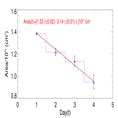
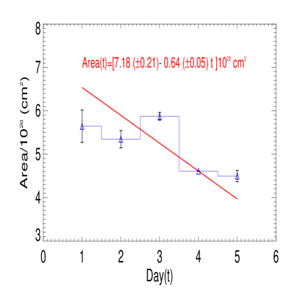
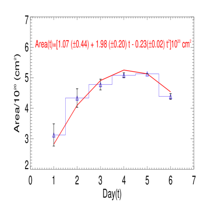
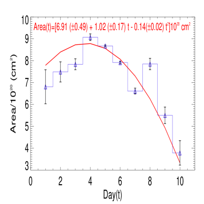
Figure 10: For different days, measured average areas of the CH (blue bar plot) that are normalized with the area $10^{20}cm^{2}$. Figures in the upper panel are the variation of areas of CH for the number of observed 4 and 5 days ($\tau$) respectively. Whereas figures in the lower panel illustrate the variation of areas of CH for the number of observed 6 and 10 days ($\tau$) respectively. $\chi^{2}$ is a measure of goodness of fit.

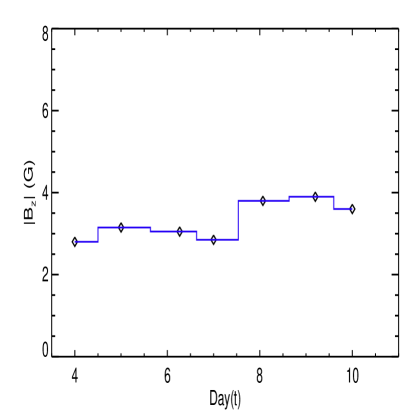
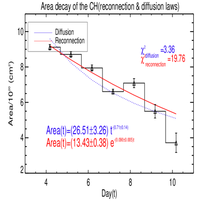
Figure 11: Variation of absolute magnitude of magnetic field structure (blue bar plot connected by diamonds; left figure) and area (black bar plot connected by triangles; right figure) of a CH for the decay part of 10 days area evolutionary curve. Areas are normalized with the area $10^{20}cm^{2}$ and are subjected to laws of magnetic diffusion ($Area(t)=A_{0}t^{-n}$, $t$ is time variable) and magnetic reconnection ($Area(t)=A_{0}e^{-c_{1}t}$) respectively. $A_{0}$, constants $n$ and $c_{1}$ are determined from the least square fit. $\chi^{2}$ is a measure of goodness of fit.

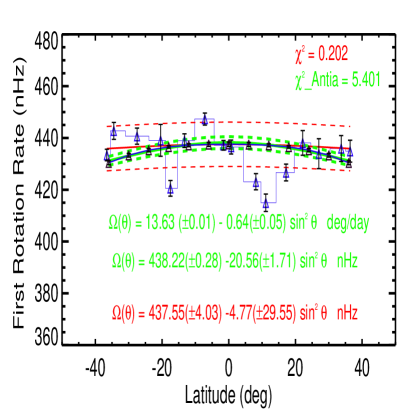
Figure 13: For all the sizes and number of observed days ($\tau$), figure illustrates first rotation rates of coronal holes (blue bar plot connected by blue triangles), with a least-square fit (red continuous line). Also plotted is the helioseismically inferred (Antia & Basu 2010) rotation rate (green continuous line connected by black triangles with green dashed lines as one sigma error bands) at a depth of $0.62(\pm 0.10)R_{\odot}$, as a function of latitude. Red and green dashed lines represent one standard deviation (that is computed from all the data points) error bands. $\chi^{2}$ is a measure of goodness of fit.

As for the anchoring depths, during their first appearance in the corona and owing to its magnetic nature (Gurman et al. 1974; Bohlin 1977; Levine 1977; Bohlin & Sheeley 1978; Stenflo 1978; Harvey & Sheeley 1979; Harvey et al. 1982; Shelke & Pande 1984; Obridko & Shelting 1989; Zhang et al. 2006; Fainshtein 2010), we expect that a coronal hole might isorotates with the solar plasma, so its rotation rate during its first appearance and the rotation rate at the anchoring depth must be identical. It is interesting to note that the average rotation rate ($\sim$ 438 nHz), we have measured in coronal holes (Fig 13) is similar to that of the average rotation rate of the solar plasma inferred by helioseismology (Antia & Basu 2010; rotation rate of the solar interior averaged over one solar cycle is kindly provided by Prof. Antia) at a depth of $\sim 0.62(\pm 0.10)R_{\odot}$. Hence, during first appearance of the coronal hole, it is reasonable to suggest that the depth of anchoring of CH might be around $0.62(\pm 0.10)R_{\odot}$. If we simply identify the rotation rates found here with the internal rotation rate at a given depth, we find a match only inside the radiative interior, at a depth of $0.62(\pm 0.10)R_{\odot}$ solar radii. In future, helioseismology may give further inferences on the anchoring depths of coronal holes. We know, however, of no currently accepted model of magnetic field generation that could anchor coronal structures to such a depth in the interior. With a caveat that unless a consistent and acceptable theoretical model of CH that supports of our proposition (that during their first appearance, roots of CH might be anchored in the radiative core), our proposed idea remains mere a conjecture only.

To conclude this study, we used SOHO/EIT 195 $\AA$ calibrated images to determine the latitudinal and day to day variations of rotation rates of the coronal holes. We found that: (1) irrespective of their areas and number of days ($\tau$) observed on the disk, for different latitude zones, rotation rates of CH follow a rigid body rotation law, (2) CH also rotate rigidly during their evolution history and, (3) during their first appearance, CH rotate rigidly with a constant angular velocity $\sim$ 438 nHz which only matches depth around $0.62(\pm 0.10)R_{\odot}$, in the radiative interior. This result is so counterintuitive that we can only conclude that we do not understand why CH rotate rigidly at that rate.

Acknowledgements

Authors are grateful to an anonymous referee for the invaluable comments and suggestions that substantially improved the results and presentation of the manuscript. Authors are also grateful to Dr. J. B. Gurman for giving useful information on the SOHO data, for going through the earlier version of this manuscript and, for giving useful ideas. Hiremath is thankful to former Director, Prof. Siraj Hasan, Indian Institute of Astrophysics, for encouraging this ISRO funded project. This work has been carried out under “CAWSES India Phase-II program of Theme 1” sponsored by Indian Space Research Organization(ISRO), Government of India. SOHO is a mission of international cooperation between ESA and NASA.

References

- [1] Aiouaz, T. 2008, ApJ, 674, 1144
- [2] Antia, H. M., Basu, S., & Chitre, S. M. 1998, MNRAS, 298, 543
- [3] Antia, H. M. & Basu, S. 2010, ApJ, 720, 494
- [4] Balthasar, H., Vazquez, M., & Woehl, H. 1986, A&A, 155, 87
- [5] Bohlin, J. D. 1977, Solar Phys, 51, 377
- [6] Bohlin, J. D. & Sheeley, N. R., Jr. 1978, Solar Phys, 56, 125
- [7] Brajša, R., Wöhl, W., Vršnak, B., Rudžjak, V., Clette, F., Hochedez, J.-F., & Roša, D. 2004, A&A, 414, 707
- [8] Brajša, R., Wöhl, W., Vršnak, B., Rudžjak., D. Sudar., Roša, D., & Hrzina, D. 2002, Solar Phys, 206, 229
- [9] Chandra, S., Vats, H. O., & Iyer, K. N. 2009, MNRAS, 400, L34
- [10] Chandra, S., Vats, H. O., & Iyer, K. N. 2010, MNRAS, 407, 1108
- [11] Choi, Y., Moon, Y.-J., Choi, S., Baek, J.-H., Kim, S. S., Cho, K.-S., & Choe, G. S. 2009, Solar Phys, 254, 311
- [12] Cranmer, S.R. 2009, Living Reviews in Solar Phys, 6, 3
- [13] Crooker, N. U. & Owens, M. J. 2011, Space Science Reviews, DOI:10.1007/s11214-011-9748-1
- [14] Dalsgaard, C. J. & Schou, J. 1988, Seismology of the Sun and Sun-like stars, ed. Rolfe, E. J., ESASP, 286, 149
- [15] Delaboudiniére, J. P. et al. 1995, Solar Phys, 162, 291
- [16] de Toma, G. 2011, Solar Phys, 274, 195
- [17] Edmondson, J. K., Antiochos, S. K., DeVore, C. R., Lynch, B. J., & Zurbuchen, T. H. 2010, ApJ, 714, 517
- [18] Fainshtein, V. G., Stepanian, N. N., Rudenko, G. V., Malashchuk, V. M., & Kashapova, L. K. 2010, Bulletin of the Crimean Astrophysical Observatory, 106, 1
- [19] Fisher, R. & Sime, D.G. 1984, ApJ, 287, 959
- [20] Freeland, S. L. & Handy, B. N. 1998, Solar Phys, 182, 497
- [21] Gilman, P. A. 1977, Coronal holes and high speed wind streams Conference, ed. Zirker, J. B. 331
- [22] Golub, L., Rosner, R., Vaiana, G. S., & Weiss, N. O. 1981, ApJ, 243, 309
- [23] Gurman, J. B., Withbroe, G. L., & Harvey, J. W. 1974, Solar Phys, 34, 105
- [24] Hansen, R.T., Hansen, S.F., & Looms, H.G. 1969, Solar Phys, 10, 135
- [25] Hara, H. 2009, ApJ, 687, 980
- [26] Harvey, J. W. & Sheeley, N. R., Jr. 1979, SSR, 23, 139
- [27] Harvey, K. L., Harvey, J. W., & Sheeley, N. R., Jr. 1982, Solar Phys, 79, 149
- [28] Hiremath, K. M. 2002, A&A, 386, 674
- [29] Hiremath, K. M. 2009, Sun and Geosphere, 4, 16
- [30] Hiremath, K. M. 2010, Sun and Geosphere, 5, 17
- [31] Hiremath, K. M. 2010, arXiv1012.5706
- [32] Hoeksema, J.T. 1984, Ph.D. Thesis, Stanford University
- [33] Howard, R. & Harvey, J. 1970, Solar Phys, 12, 23
- [34] Howard, R. & La Bonte, B. J. 1980, ApJ, 239, L33
- [35] Howard, R., Gilman, P. I., & Gilman, P. A. 1984, ApJ, 283, 373
- [36] Howe, R. 2009, Living Review in Solar Phys, 6, 1
- [37] Insley, J.E., Moore, V., & Harrison, R.A. 1995, Solar Phys, 160, 1
- [38] Javaraiah, J. 2003, Solar Phys, 212, 23
- [39] Jones, H. P. 2005, Large-scale Structures and their Role in Solar Activity ASP Conference, eds, Sankarasubramanian, K., Penn, M., & Pevtsov, A. 346, 229
- [40] Kahler, S. W. & Hudson, H. S. 2002, ApJ, 574, 467
- [41] Kahler, S., Jibben, P., & Deluca, E. E. 2010, Solar Phys, 262, 135
- [42] Kariyappa, R. 2008, A&A, 488, 297
- [43] Karachik, N. V., Pevtsov, A. A., & Sattarov, I. 2006, ApJ, 642, 562
- [44] Karachik, N. V., Pevtsov, A. A., & Abramenko, V. I. 2010, ApJ, 714, 1672
- [45] Karachik, N. V. & Pevtsov, A. A. 2011, ApJ, 735, 47
- [46] Komm, R. W., Howard, R. F., & Harvey, J. W. 1993, Solar Phys, 145, 1
- [47] Krieger, A.S., Timothy, A.F., & Roelof, E.C. 1973, Solar Phys, 29, 505
- [48] Krista, L. D. & Gallagher, P.T. 2009, Solar Phys, 256, 87
- [49] Krista, L. D. 2011, Ph.D Thesis, University of Dublin, Trinity College
- [50] Krista, L. D., Gallagher, P. T., & Bloomfield, D. S. 2011, ApJ, 731, 26
- [51] Levine, R. H. 1977, ApJ, 218, 291
- [52] Lei, J., Thayer, J. P., Forbes, J. M., Sutton, E. K., & Nerem, R. S. 2008, Geophys Res Let, 35, L19105
- [53] Li, K. J., Shi, X. J., Feng, W., Xie, J. L., Gao, P. X., Zhan, L. S., & Liang, H. F. 2012, MNRAS, 2012, DOI: 10.1111/j.1365-2966.2012.21155.x
- [54] Madjarska, M. S., Doyle, J. G. & van Driel-Gesztelyi, L. 2004, ApJ, 603, L57
- [55] Madjarska, M. S. & Wiegelmann, T. 2009, A&A, 503, 991
- [56] Madjarska, M. S., Huang, Z., Doyle, J. G., & Subramanian, S. 2012, A&A, 545, A67
- [57] Mancuso, S. & Giordano, S. 2011, ApJ, 729, 79
- [58] Navarro-Peralta, P. & Sanchez-Ibarra, A. 1994, Solar Phys, 153, 169
- [59] Neupert, W.M. & Pizzo, V. 1974, J. Geophys. Res., 79, 3701
- [60] Newton, H. W. & Nunn, M. L. 1951, MNRAS, 111, 413
- [61] Nolte, J. T., Krieger, A. S., Timothy, A. F., Gold, R. E., Roelof, E. C., Vaiana, G., Lazarus, A. J., Sullivan, J. D., & McIntosh, P. S. 1976, 46, 303
- [62] Parker, G. D., Hansen, R.T., & Hansen, S.F. 1982, Solar Phys, 80, 185
- [63] Pevtsov, A. A. & Abramenko, V. I. 2010, Solar and Stellar Variability: Impact on Earth and Planets, Proceedings of the International Astronomical Union, eds. Kosovichev, A. G., Andrei, A. H., & Rozelot, J.-P. 264, 210
- [64] Obridko, V. N. & Shelting, B. D. 1989, Solar Phys, 124, 73
- [65] Raju, K. P., Bromage, B. J. I., Chapman, S. A., & Del Zanna, G. 2005, A&A, 432, 341
- [66] Ram, S. T., Liu, C. H., & S.-Y. Su. 2010, JGR, 115, 14
- [67] Roša, D., Brajša, R., Vršnak, B., & Wöhl, H. 2005, Solar Phys, 159, 393
- [68] Shelke, R. N. & Pande, M. C. 1984, Bull. Astron. Soc. India, 12, 404
- [69] Shelke, R. N. & Pande, M. C. 1985, Solar Phys, 95, 193
- [70] Shugai, Yu. S., Veselovsky, I. S., & Trichtchenko, L. D. 2009, Ge&Ae, 49, 415
- [71] Shivaraman, K. R., Gupta, S. S., & Howard, R. F. 1993, Solar Phys, 146, 2
- [72] Snodgrass, H. B. 1983, ApJ, 270, 288
- [73] Snodgrass, H. B. & Ulrich, R. K. 1990, ApJ, 351, 309
- [74] Snodgrass, H. B. 1992, The Solar Cycle, ed. Harvery, K.L. ASP Conf. Ser, 27, 205
- [75] Sojka, J. J., McPherron, R. L., van Eyken, A. P., Nicolls, M. J., Heinselman, C. J., & Kelly, J. D. 2009, Geophys Res Let, 36, L19105
- [76] Soon, W., Baliunas, S., Posmentier, E. S., & Okeke, P. 2000, New Astronomy, 4, 563
- [77] Stenflo, J. O. 1978, Reports on Progress in Physics, 41, 865
- [78] Subramanian, S., Madjarska, M. S., & Doyle, J. G. 2010, A&A, 516, A50
- [79] Thompson, M. J. et al. 1996, Science, 272, 1300
- [80] Thompson, M. J., Dalsgaard, C. J., Miesch, M. S., & Toomre, J. 2003, AAPR, 41, 599
- [81] Tian, H., McIntosh, S. W., Habbal, S. R., & He, J. 2011, ApJ, 736, 130
- [82] Timothy, A. F. & Krieger, A. S. 1975, Solar Phys, 42, 135
- [83] Ulrich, R. K., Boyden, J. E., Webster, L., & Shieber, T. 1988, Seismology of the Sun and Sun-Like Stars, ed, Rolfe, E. J., ESASP, 286, 325
- [84] Verbanac, G., Vršnak, B., Veronig, A., & Temmer, M. 2011, A&A, 526, 20
- [85] Wagner, W. J. 1975, ApJ, 198L, 141
- [86] Wagner, W. J. 1976, Basic Mechanisms of Solar Activity, Proceedings from IAU Symposium no. 71, edts. Bumba, V and Kleczek, J, p. 41
- [87] Wang, Y.M., Sheeley, N. R., Jr., Nash, A. G., & Sampine, L. R. 1988, ApJ, 327, 427
- [88] Wang, Y.M., Space Sci Rev, 2009, 144, 383
- [89] Weber, M. A., Acton, L. W., Alexander, D., Kubo, S., & Hara, H. 1999, Solar Phys, 189, 271
- [90] Weber, M. A. & Sturrock, P. A. 2002, Multi-Wavelength Observations of Coronal Structure and Dynamics – Yohkoh 10th Anniversary Meeting. eds. Martens, P. C. H. & Cauffman, D. 347
- [91] Wilcox, J. M. & Howard, R. 1970, Solar Phys, 13, 251
- [92] Wiitmann, A. D. 1996, Solar Phys, 168, 211
- [93] Wöhl, H., Brajša, R., Hanslmeier, A., & Gissot, S. F. 2010, A&A, 520, 29
- [94] Yang, S.-H., Zhang, J., Li, T., & Liu, Y. 2011, ApJ, 732, L7
- [95] Zhang, J., Jun, M., & Wang, H. 2006, ApJ, 649, 464
- [96] Zirker, J. B. 1977, Reviews of Geophysics and Space Physics, 15, 257