Magic wavelengths for trapping the alkali-metal atoms with circularly polarized light

Abstract

Magic wavelengths for the Li, Na and K alkali atoms are determined using the circulalrly polarized light for the $ns-np_{1/2,3/2}$ transitions, with $n$ denoting their ground state principal quantum numbers, by studying their differential ac dynamic polarizabilities. These wavelengths for all possible sub-levels are given linearly as well as circulalrly polarized lights and are further compared with the available results for the linearly polarized light. The present study suggests that it is possible to carry out state insensitive trapping of different alkali atoms using the circularly polarized light.

I Introduction

It has been known for some time that atoms can be trapped and manipulated by the gradient forces of light waves Kazantsev et al. (1990); Grimm et al. (2000); Balykin et al. (2000). However, for any two internal states of an atom, the Stark shifts caused due to the trap light are different which affects the fidelity of the experiments Safronova et al. (2003); Takamoto and Katori (2003). Katori et al. Katori et al. (1999) suggested a solution to this problem that the trapping laser can be tuned to wavelength, “$\lambda_{\rm{magic}}$”, where the differential ac Stark shifts of the transition vanishes. Knowledge of magic wavelengths is necessary in many areas of physics. In particular, these wavelengths have unavoidable application for atomic clocks and quantum computing Katori (2002); Sackett et al. (2000). For example, a major concern for the accuracy of optical lattice clocks is the ability to cancel the large light shifts created by the trapping potential of the lattice. Similarly, for most of the quantum computational schemes, it is often desirable to optically trap the neutral atoms without affecting the internal energy-level spacing for the atoms.

Over the years, there has been quite a large number of calculations of the magic wavelengths of alkali-metal atoms for linearly polarized traps Ludlow and et al. (2005); McKeever et al. (2003); Arora et al. (2007), with rather fewer calculations of the magic wavelength for the circularly polarized traps. Moreover, as stated in Arora et al. (2007), the linearly polarized lattice scheme offers only a few cases in which the magic wavelengths are of experimental relevance. Therefore, we would like to explore the idea of using the circularly polarized light. Using the circularly polarized light may be advantageous owing to the dominant role played by vector polarizabilities in estimating the ac Stark shifts Arora and Sahoo (2012); Flambaum et al. (2008); Park et al. (2001). These polarizability contributions are absent in the linearly polarized light. Recently, we had investigated the magic wavelengths for the circularly polarized light in rubidium (Rb) atom and found spectacular results that can lead to state insensitive trapping of Rb atoms using this light Arora and Sahoo (2012). In this paper, we aim at searching for magic wavelengths in the Li, Na, and K atoms due to circularly polarized light and also compare our results for linearly polarized light with other available results.

II Theory

The energy shift of any state $v$ of an atom placed in a frequency-dependent ac electric field $\mathcal{E}(\omega)$, can be estimated from the time-independent perturbation theory at the second order perturbation level as

$$\Delta E_{v}\simeq-\frac{1}{2}\alpha_{v}(\omega)\mathcal{E}^{2},$$ (1)

where $\alpha_{v}(\omega)$ is the dynamic dipole polarizability of the atom in the $v^{th}$ state and can be expressed as

$$\alpha_{v}(\omega)=-\sum_{k\neq v}({p^{*}})_{vk}({p})_{kv}\left[\frac{1}{\delta E_{vk}+\omega}+\frac{1}{\delta E_{vk}-\omega}\right],$$ (2)

where $({p})_{kv}={\left\langle\psi_{k}\left|D\right|\psi_{v}\right\rangle}$ is the electric-dipole matrix element. In a more conventional form, the dipole polarizability $\alpha(\omega)$ can be decomposed into three components as

$$\alpha_{v}(\omega) = \alpha_{v}^{0}(\omega)+\mathcal{A}\cos{\theta_{k}}\frac{m_{j}}{j}\alpha_{v}^{1}(\omega)$$ (3)

$$+\left\{\frac{3\cos^{2}{\theta_{p}}-1}{2}\right\}\frac{3m_{j}^{2}-j(j+1)}{j(2j-1)}\alpha_{v}^{2}(\omega),$$

which separates out the $m_{j}$ dependent and independent components. The $m_{j}$ independent parameters $\alpha_{0}(\omega)$, $\alpha_{1}(\omega)$ and $\alpha_{2}(\omega)$ are known as scalar, vector and tensor polarizabilities, respectively. They are given in terms of the reduced matrix dipole matrix elements as Manakov et al. (1986)

$$\alpha_{v}^{0}(\omega) = \frac{1}{{3(2j_{v}+1)}}\sum_{j_{k}}|\langle\psi_{v}\parallel D\parallel\psi_{k}\rangle|^{2}$$ (4)

$$\times\left[\frac{1}{\delta E_{kv}+\omega}+\frac{1}{\delta E_{kv}-\omega}\right],$$

$$\alpha_{v}^{1}(\omega) = -\sqrt{\frac{6j_{v}}{(j_{v}+1)(2j_{v}+1)}}\sum_{j_{k}}\left\{\begin{array}[]{ccc}j_{v}&1&j_{v}\\ 1&j_{k}&1\end{array}\right\}$$ (8)

$$(-1)^{j_{v}+j_{k}+1}|\langle\psi_{v}\parallel D\parallel\psi_{k}\rangle|^{2}$$

$$\times\left[\frac{1}{\delta E_{kv}+\omega}-\frac{1}{\delta E_{kv}-\omega}\right]$$

and

$$\alpha_{v}^{2}(\omega) = -2\sqrt{\frac{5j_{v}(2j_{v}-1)}{6(j_{v}+1)(2j_{v}+1)(2j_{v}+3)}}$$ (12)

$$\sum_{j_{k}}\left\{\begin{array}[]{ccc}j_{v}&2&j_{v}\\ 1&j_{k}&1\end{array}\right\}(-1)^{j_{v}+j_{k}+1}|\langle\psi_{v}\parallel D\parallel\psi_{k}\rangle|^{2}$$

$$\times\left[\frac{1}{\delta E_{kv}+\omega}+\frac{1}{\delta E_{kv}-\omega}\right].$$

In the above expression $\mathcal{A}$, $\theta_{k}$ and $\theta_{p}$ define degree of circular polarization, angle between wave vector of the electric field and $z$-axis and angle between the direction of polarization and $z$-axis, respectively. Without the loss of generality, it is assumed that the considered frequencies ($\omega$s) are several line-widths off from the resonance lines and $\mathcal{A}=1$ for the right-handed and $\mathcal{A}=-1$ for the left-handed circularly polarized light. In the absence of the magnetic field (or in weak magnetic field), we approximate $\cos(\theta_{k})=\cos(\theta_{p})=1$.

The differential ac Stark shift for a transition is defined as the difference between the Stark shifts of individual levels which are further calculated from the frequency-dependent polarizabilities:

$$\delta(\Delta E)_{np_{i}-ns} = \Delta E_{np_{i}}-\Delta E_{ns}$$ (13)

$$= \frac{1}{2}\mathcal{E}^{2}(\alpha_{ns}-\alpha_{np_{i}}),$$

where we have used the total polarizabilities of the respective states and $i=1/2,3/2$. Since the external electric field $\mathcal{E}$ is arbitrary, we can locate the frequencies or wavelengths where $\alpha_{np_{i}}=\alpha_{ns}$, for an atom for the null differential ac Stark shifts which gives the value of magic wavelengths. In other words, the crossing between the two polarizabilities at various values of wavelengths will correspond to $\lambda_{\rm{magic}}$. As pointed out in the begining, it will be experimentally convenient to trap atoms at these wavelengths.

III Procedure for calculations

The scalar, vector and tensor polarizabilities can be written using sum-over intermediate states as

$$\alpha_{v}^{\lambda} = \sum_{j_{k}}C_{v,k}^{\lambda}\frac{|\langle j_{v}||D||j_{k}\rangle|^{2}}{E_{v}-E_{k}},$$ (14)

where $\lambda=0,\ 1$ and $2$ represents for scalar, vector and tensor polarizabilities and $C_{v,k}^{\lambda}$ are their corresponding angular coefficients. In order to apply this formula, it is necessary to determine intermediate $k$ states explicitly. Therefore, contributions from the intermediate states involving core orbitals cannot be determined in this procedure. For a practical approach, we divide contributions to $\alpha_{v}$ as

$$\alpha_{v}^{\lambda} = \alpha_{v}^{\lambda}(c)+\alpha_{v}^{\lambda}(vc)+\alpha_{v}^{\lambda}(v),$$ (15)

by expressing wave functions of the state $v$ as a closed core with the corresponding valence orbital so that $\alpha_{v}^{\lambda}(c)$ and $\alpha_{v}^{\lambda}(vc)$ account contributions from the intermediate states involving core orbitals and $\alpha_{v}^{\lambda}(v)$ take care of the contributions from the excited states involving the virtual orbitals. As a result, $\alpha_{v}^{\lambda}(v)$ contributions will be the dominant ones among them and and can be estimated determining the important low-lying intermediate states explicitly. Contributions from $\alpha_{v}^{\lambda}(c)$, $\alpha_{v}^{\lambda}(vc)$ and higher intermediate states with the virtual orbitals (given as $tail$ contributions) are obtained using the third order many-body perturbation theory (MBPT(3) method) in the Lewis-Galgarno approach Arora and Sahoo (2012); Arora et al. (2012).

To determine contributions to $\alpha_{v}^{\lambda}(v)$ from the low-lying intermediate states involving virtual orbitals, we express atomic wave functions of a given state with a colsed core and a valence orbital $k$ as

$$|\Phi_{k}\rangle=a_{k}^{\dagger}|\Phi_{0}\rangle,$$ (16)

where $|\Phi_{0}\rangle$ is the Dirac-Fock (DF) wave function for the closed core and $a_{k}^{\dagger}$ correspond to the attachment of the $k$ valence orbital to the core. The wave function of the exact state is then expressed in the coupled-cluster (CC) theory framework as Lindgren (1978)

$$|\Psi_{v}\rangle = e^{T}\{1+S_{v}\}|\Phi_{v}\rangle,$$ (17)

where $T$ and $S_{v}$ operators account coorelation effects from core and core with valence orbitals, respectively. Amplitudes of these operators are obtained using the Dirac-Coulomb (DC) Hamiltonian and the detailed procedures are explained else where (e.g. refer to Mukherjee et al. (2009); Sahoo et al. (2004)).

Table 1: Absolute values of E1 matrix elements in Li, Na, and K atoms in $ea_{0}$ using CCSD(T) methods. Uncertainties in the CCSD(T) results are given in the parentheses.

Transition	CCSD(T)	Transition	CCSD(T)
Li
$2s_{1/2}\rightarrow 2p_{1/2}$	3.318(4)	$2p_{1/2}\rightarrow 5d_{3/2}$	1.212(1)
$2s_{1/2}\rightarrow 3p_{1/2}$	0.182(2)	$2p_{1/2}\rightarrow 6d_{3/2}$	0.767(1)
$2s_{1/2}\rightarrow 4p_{1/2}$	0.159(2)	$2p_{1/2}\rightarrow 7d_{3/2}$	0.566(5)
$2s_{1/2}\rightarrow 5p_{1/2}$	0.119(4)	$2p_{3/2}\rightarrow 3s_{1/2}$	3.445(3)
$2s_{1/2}\rightarrow 6p_{1/2}$	0.092(2)	$2p_{3/2}\rightarrow 4s_{1/2}$	0.917(2)
$2s_{1/2}\rightarrow 7p_{1/2}$	0.072(1)	$2p_{3/2}\rightarrow 5s_{1/2}$	0.493(2)
$2s_{1/2}\rightarrow 2p_{3/2}$	4.692(5)	$2p_{3/2}\rightarrow 6s_{1/2}$	0.326(2)
$2s_{1/2}\rightarrow 3p_{3/2}$	0.257(2)	$2p_{3/2}\rightarrow 7s_{1/2}$	0.233(2)
$2s_{1/2}\rightarrow 4p_{3/2}$	0.225(2)	$2p_{3/2}\rightarrow 3d_{3/2}$	2.268(2)
$2s_{1/2}\rightarrow 5p_{3/2}$	0.169(4)	$2p_{3/2}\rightarrow 4d_{3/2}$	0.863(1)
$2s_{1/2}\rightarrow 6p_{3/2}$	0.130(2)	$2p_{3/2}\rightarrow 5d_{3/2}$	0.502(1)
$2s_{1/2}\rightarrow 7p_{3/2}$	0.102(1)	$2p_{3/2}\rightarrow 6d_{3/2}$	0.344(1)
$2p_{1/2}\rightarrow 3s_{1/2}$	2.436(3)	$2p_{3/2}\rightarrow 7d_{3/2}$	0.253(4)
$2p_{1/2}\rightarrow 4s_{1/2}$	0.648(3)	$2p_{3/2}\rightarrow 3d_{5/2}$	6.805(1)
$2p_{1/2}\rightarrow 5s_{1/2}$	0.349(3)	$2p_{3/2}\rightarrow 4d_{5/2}$	2.589(1)
$2p_{1/2}\rightarrow 6s_{1/2}$	0.231(2)	$2p_{3/2}\rightarrow 5d_{5/2}$	1.505(1)
$2p_{1/2}\rightarrow 7s_{1/2}$	0.165(2)	$2p_{3/2}\rightarrow 6d_{5/2}$	1.031(1)
$2p_{1/2}\rightarrow 3d_{3/2}$	5.072(1)	$2p_{3/2}\rightarrow 7d_{5/2}$	0.746(5)
$2p_{1/2}\rightarrow 4d_{3/2}$	1.929(1)
Na
$3s_{1/2}\rightarrow 3p_{1/2}$	3.545(3)	$3p_{1/2}\rightarrow 5d_{3/2}$	0.997(2)
$3s_{1/2}\rightarrow 4p_{1/2}$	0.304(2)	$3p_{1/2}\rightarrow 6d_{3/2}$	0.645(1)
$3s_{1/2}\rightarrow 5p_{1/2}$	0.107(1)	$3p_{1/2}\rightarrow 7d_{3/2}$	0.460(1)
$3s_{1/2}\rightarrow 6p_{1/2}$	0.056(2)	$3p_{3/2}\rightarrow 4s_{1/2}$	5.070(4)
$3s_{1/2}\rightarrow 7p_{1/2}$	0.035(2)	$3p_{3/2}\rightarrow 5s_{1/2}$	1.072(2)
$3s_{1/2}\rightarrow 8p_{1/2}$	0.026(2)	$3p_{3/2}\rightarrow 6s_{1/2}$	0.553(2)
$3s_{1/2}\rightarrow 3p_{3/2}$	5.012(4)	$3p_{3/2}\rightarrow 7s_{1/2}$	0.360(1)
$3s_{1/2}\rightarrow 4p_{3/2}$	0.434(2)	$3p_{3/2}\rightarrow 8s_{1/2}$	0.255(1)
$3s_{1/2}\rightarrow 5p_{3/2}$	0.153(2)	$3p_{3/2}\rightarrow 3d_{3/2}$	3.048(3)
$3s_{1/2}\rightarrow 6p_{3/2}$	0.081(2)	$3p_{3/2}\rightarrow 4d_{3/2}$	0.856(2)
$3s_{1/2}\rightarrow 7p_{3/2}$	0.051(2)	$3p_{3/2}\rightarrow 5d_{3/2}$	0.445(2)
$3s_{1/2}\rightarrow 8p_{3/2}$	0.037(2)	$3p_{3/2}\rightarrow 6d_{3/2}$	0.288(1)
$3p_{1/2}\rightarrow 4s_{1/2}$	3.578(4)	$3p_{3/2}\rightarrow 7d_{3/2}$	0.205(1)
$3p_{1/2}\rightarrow 5s_{1/2}$	0.758(3)	$3p_{3/2}\rightarrow 3d_{5/2}$	9.144(4)
$3p_{1/2}\rightarrow 6s_{1/2}$	0.391(2)	$3p_{3/2}\rightarrow 4d_{5/2}$	2.570(3)
$3p_{1/2}\rightarrow 7s_{1/2}$	0.255(2)	$3p_{3/2}\rightarrow 5d_{5/2}$	1.336(2)
$3p_{1/2}\rightarrow 8s_{1/2}$	0.180(1)	$3p_{3/2}\rightarrow 6d_{5/2}$	0.864(2)
$3p_{1/2}\rightarrow 3d_{3/2}$	6.807(3)	$3p_{3/2}\rightarrow 7d_{5/2}$	0.606(2)
$3p_{1/2}\rightarrow 4d_{3/2}$	1.916(2)
K
$4s_{1/2}\rightarrow 4p_{1/2}$	4.131(20)	$4p_{1/2}\rightarrow 6d_{3/2}$	0.293(5)
$4s_{1/2}\rightarrow 5p_{1/2}$	0.282(6)	$4p_{1/2}\rightarrow 7d_{3/2}$	0.261(4)
$4_{1/2}\rightarrow 6p_{1/2}$	0.087(5)	$4p_{1/2}\rightarrow 8d_{3/2}$	0.221(4)
$4s_{1/2}\rightarrow 7p_{1/2}$	0.041(5)	$4p_{3/2}\rightarrow 5s_{1/2}$	5.524(10)
$4s_{1/2}\rightarrow 8p_{1/2}$	0.023(3)	$4p_{3/2}\rightarrow 6s_{1/2}$	1.287(10)
$4s_{1/2}\rightarrow 9p_{1/2}$	0.016(3)	$4p_{3/2}\rightarrow 7s_{1/2}$	0.677(6)
$4s_{1/2}\rightarrow 4p_{3/2}$	5.841(20)	$4p_{3/2}\rightarrow 9s_{1/2}$	0.317(5)
$4s_{1/2}\rightarrow 5p_{3/2}$	0.416(6)	$4p_{3/2}\rightarrow 10s_{1/2}$	0.242(5)
$4s_{1/2}\rightarrow 6p_{3/2}$	0.132(6)	$4p_{3/2}\rightarrow 3d_{3/2}$	3.583(20)
$4s_{1/2}\rightarrow 7p_{3/2}$	0.064(5)	$4p_{3/2}\rightarrow 4d_{3/2}$	0.088(5)
$4s_{1/2}\rightarrow 8p_{3/2}$	0.038(3)	$4p_{3/2}\rightarrow 5d_{3/2}$	0.124(5)
$4s_{1/2}\rightarrow 9p_{3/2}$	0.027(3)	$4p_{3/2}\rightarrow 6d_{3/2}$	0.135(5)
$4p_{1/2}\rightarrow 5s_{1/2}$	3.876(10)	$4p_{3/2}\rightarrow 7d_{3/2}$	0.119(4)
$4p_{1/2}\rightarrow 6s_{1/2}$	0.909(10)	$4p_{3/2}\rightarrow 8d_{3/2}$	0.101(3)
$4p_{1/2}\rightarrow 7s_{1/2}$	0.479(5)	$4p_{3/2}\rightarrow 3d_{5/2}$	10.749(50)
$4p_{1/2}\rightarrow 8s_{1/2}$	0.316(5)	$4p_{3/2}\rightarrow 4d_{5/2}$	0.260(5)
$4p_{1/2}\rightarrow 9s_{1/2}$	0.225(3)	$4p_{3/2}\rightarrow 5d_{5/2}$	0.374(5)
$4p_{1/2}\rightarrow 10s_{1/2}$	0.171(3)	$4p_{3/2}\rightarrow 6d_{5/2}$	0.404(5)
$4p_{1/2}\rightarrow 3d_{3/2}$	7.988(40)	$4p_{3/2}\rightarrow 7d_{5/2}$	0.356(5)
$4p_{1/2}\rightarrow 4d_{3/2}$	0.220(5)	$4p_{3/2}\rightarrow 8d_{5/2}$	0.286(5)
$4p_{1/2}\rightarrow 5d_{3/2}$	0.264(5)

Table 2: Comparision of polarizabilities of the ground and first two excited states in Li, Na and K (a.u.) from this work with the results reported in Safronova et al. (2012)^a, Miffre et al. (2006)^b, Derevianko et al. (1999)^c, Arora et al. (2007)^d, Ekstrom et al. (1995)^e, Windholz and Musso (1989)^f, ^gRef. Holmgren et al. (2010),^hderived from Ref. Miller et al. (1994) D1 line Stark shift measurements and recommended values for ground state polarizability from Ref. Derevianko et al. (1999),ⁱRef. Krenn et al. (1997).

.

Contributions	$ns$	$np_{1/2}$	$np_{3/2}$
from	$\alpha_{v}^{0}$	$\alpha_{v}^{0}$	$\alpha_{v}^{0}$	$\alpha_{v}^{2}$
Li ($n=2$)
$2s$	-	-54.041(4)	-54.031(5)	54.031(5)
$2p_{1/2}$	54.041(4)	-	-	-
$2p_{3/2}$	108.06(1)	-	-	-
$3s$	-	35.288(2)	35.288(2)	-35.288(2)
$3p_{1/2}$	0.078	-	-	-
$3p_{3/2}$	0.156	-	-	-
$3d_{3/2}$	-	114.901(2)	11.488(1)	9.190
$3d_{5/2}$	-	-	103.419(2)	-20.684
$4s$	-	1.528()	1.530	-1.530
$4p_{1/2}$	0.051	-	-	-
$4p_{3/2}$	0.102	-	-	-
$4d_{3/2}$	-	12.534(1)	1.254	-2.258
$4d_{5/2}$	-	-	11.289	-2.258
$\alpha_{v}(v)$	0.154	7.63	6.931	-0.627
$\alpha_{v}(cv)$	$\sim 0$	$\sim 0$	$\sim 0$	$\sim 0$
$\alpha_{v}(tail)$	1.2(6)	10(5)	10(5)	-1.7(8)
Present	164.1(6)	128	127	1.5
Others	164.16(5)a	126.97(5)a	126.98(5)a	1.610(26)a
Expt.	164.2(11)b	-	-	-
Na ($n=3$)
3s	-	-53.60(7)	-53.53(7)	53.53(7)
${\bf 3p_{1/2}}$	53.60(7)	-	-	-
${\bf 3p_{3/2}}$	107.06(15)	-	-	-
$4s$	-	106.625(9)	107.255(9)	-107.255(9)
$3d_{3/2}$	-	277.47(2)	27.856(2)	22.285(1)
$3d_{5/2}$	-	-	250.71(2)	-50.141(4)
$4p_{1/2}$	0.223	-	-	-
$4p_{3/2}$	0.455	-	-	-
$5s$	-	2.588	2.591	-2.591
$5p_{1/2}$	0.024	-	-	-
$5p_{3/2}$	0.049	-	-	-
$4d_{3/2}$	-	15.266(1)	1.525	1.220
$4d_{5/2}$	-	-	13.747	-2.749
$\alpha_{v}(v)$	0.030	6.647	6.616	-1.479
$\alpha_{v}(cv)$	$\sim 0$	$-1.3$x $10^{-4}$	$-2.6$ x $10^{-4}$	$\sim 0$
$\alpha_{v}(tail)$	0.08(4)	5(3)	5(3)	-1.5(7)
Present	162.4(2)	361	362	-88
Others	162.6(3)c	359.9d	361.6d	-88.4d
Expt.	162.7(8)e	359.2(6)e	360.4(7)e	-88.3(4)f
K ($n=4$)
${\bf 4s}$	-	-94.8(2)	-94.3(3)	94.3(3)
${\bf 4p_{1/2}}$	94.8(2)	-	-	-
${\bf 4p_{3/2}}$	188.7(5)	-	-	-
$5s$	-	0.027	139.81(3)	-139.81(3)
$3d_{3/2}$	-	545.9(4)	55.29(2)	44.23(2)
$3d_{5/2}$	-	-	497.7(5)	-99.54(10)
$5p_{1/2}$	0.236	-	-	-
$5p_{3/2}$	0.512	-	-	-
$4d_{3/2}$	-	0.246	0.020	0.016
$4d_{5/2}$	-	-	0.172	-0.035
$6s$	-	4.179(1)	4.205(1)	-4.205(1)
$6p_{1/2}$	0.019	-	-	-
$6p_{3/2}$	0.044	-	-	-
$5d_{3/2}$	-	0.296	0.033	0.026
$5d_{5/2}$	-	-	0.299	-0.060
$\alpha_{v}(v)$	0.020	2.421	2.444	-3.160
$\alpha_{v}(cv)$	-0.13	$\sim 0$	$\sim 0$	$\sim 0$
$\alpha_{v}(tail)$	0.06(3)	6.1(6)	6.2(6)	-2.1(4)
Present	289.8(6)	605.3	616.0	-107.5
Others	290.2(8)c	602d	613d	-109d
Expt.	290.58(1.42)g	606.7(6)h	614(10)i	107(2)i

We calculate the reduced matrix elements of $D$ between states $|\Psi_{f}\rangle$ and $|\Psi_{i}\rangle$ after obtaining from the above procedure that to be used in the sum-over-states approach as expression

$$\langle\Psi_{f}||D||\Psi_{i}\rangle = \frac{\langle\Phi_{f}||\{1+S_{f}^{\dagger}\}\overline{D}\{1+S_{i}\}||\Phi_{i}\rangle}{\sqrt{{\cal N}_{f}{\cal N}_{i}}},$$ (18)

where $\overline{D}=e^{T^{\dagger}}De^{T}$ and ${\cal N}_{v}=\langle\Phi_{v}|e^{T^{\dagger}}e^{T}+S_{v}^{\dagger}e^{T^{\dagger}}e^{T}S_{v}|\Phi_{v}\rangle$. Detailed calculation procedures of these expressions are discussed elsewhere Mukherjee et al. (2009); Sahoo et al. (2004).

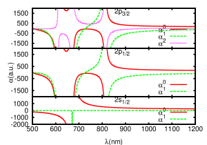
Figure 1: (color online)Scalar $\alpha^{0}$, vector $\alpha^{1}$ and tensor $\alpha^{2}$ polarizability (in a.u.) for $2s_{1/2}$, $2p_{1/2}$ and $2p_{3/2}$ state of Li atom as a function of wavelength (in n.m.)

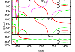
Figure 2: (color online) Scalar $\alpha^{0}$, vector $\alpha^{1}$ and tensor $\alpha^{2}$ polarizability (in a.u.) for $3s_{1/2}$, $3p_{1/2}$ and $3p_{3/2}$ state of Na atom as a function of wavelength (in n.m.)

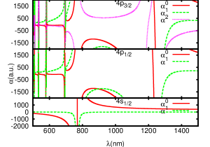
Figure 3: (color online) Scalar $\alpha^{0}$, vector $\alpha^{1}$ and tensor $\alpha^{2}$ polarizability (in a.u.) for $4s_{1/2}$, $4p_{1/2}$ and $4p_{3/2}$ state of K atom as a function of wavelength (in n.m.)

IV Results and Discussion

We first use the obtained E1 matrix elements and other MBPT(3) results to evaluate static polarizabilities ($\omega=0$) of the considered states in Li, Na and K to bench mark their accuracies aganist the previously reported experimental and theoretical results. The matrix elements calculated using the method mentioned above are shown in Table 1 and are presented under the column CCSD(T). Uncertainties in the E1 matrix elements and MBPT(3) results are estimated using the procedures given in Arora and Sahoo (2012); Nandy et al. (2012). To reduce the uncertainties in our calculations, we have taken the E1 matrix elements complied in Ref. Volz and Schmoranzer (1996), they are pointed out in the table explicitly, instead from our calculations. Experimental energies from the national institute of science and technology (NIST) database Moore (1971); Kramida et al. (2012); Sansonetti et al. (2005) are used in the present calculations. The determined polarizabilities are given in Table 2 and compared with the other results. The most accurate experimental measurement of Li ground state polarizability $\alpha_{2s}^{0}=164.2(11)$ a.u. was obtained in Miffre et al. (2006). Our result $\alpha_{2s}^{0}=164(1)$ a.u. is in excellent agreement with the experimental value. The most strigent experimental value for Na ground state polarizabilitty was obtained by interferometry experiment as $\alpha_{3s}^{0}=162.7(8)$ a.u. Ekstrom et al. (1995) and our present value $\alpha_{3s}^{0}=162.4(2)$ a.u. agrees well with the experimental value within the uncertainty limits. The most recent experimental result available for the ground state polarizability in K is $\alpha_{4s}^{0}=290.58(1.42)$ a.u.  Holmgren et al. (2010), which is very close to our calculated value $\alpha_{4s}^{0}=289.8(6)$ a.u. Our results for all the states in the considered three atoms also agree with other theoretical results. Therefore, the present polarizability results can be used further to find out magic wavelengths in these atoms.

To find magic wavelengths, i.e. the null differenial dynamic polarizabilities among various states, we first determine the frequency dependent polarizabilities. In Figs. 1, 2, and 3, we present these results for the scalar, vector and tensor polarizabilities for Li, Na, and K atoms, respectively. In Figs. 4, 5, and 6 we plot the total dynamic polarizability for the $ns$ and $np_{3/2}$ states of Li, Na, and K atoms respectively (where $n=2$ for Li, $n=3$ for Na and $n=4$ for K). In the case of the $np_{3/2}$ states, the total polarizability in the presence of linearly polarized light, is determined as $\alpha=\alpha_{0}-\alpha_{2}$ for $m_{j}=\pm 1/2$ and $\alpha=\alpha_{0}+\alpha_{2}$ for $m_{j}=\pm 3/2$. Similarly, the total polarizability for the $np_{3/2}$ states due to the circularly polarized light is determined separately for the $m_{j}=-3/2,-1/2,1/2,3/2$ sublevels using Eq.(3). Magic wavelengths for the corresponding transitions are located at the crossing of the two curves.

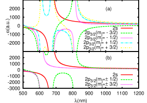
Figure 4: (color online)Total dynamic polarizability for $2s$ and $2p_{3/2}$ states of Li atom due to (a) linearly polarized light (b) circularly polarized light. Magic wavelength for the corresponding $2s-2p_{3/2}$ transition are given by the crossing of two polarizability curves.

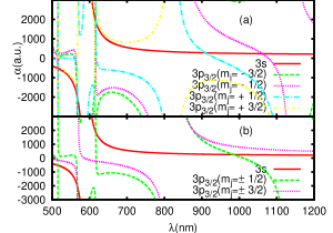
Figure 5: (color online) Total dynamic polarizability for $3s$ and $3p_{3/2}$ states of Na atom due to (a) linearly polarized light (b) circularly polarized light. Magic wavelength for the corresponding $3s-3p_{3/2}$ transition are given by the crossing of two polarizability curves.

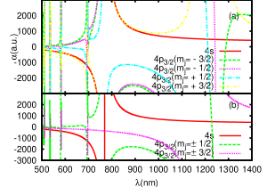
Figure 6: (color online) Total dynamic polarizability for $4s$ and $4p_{3/2}$ states of K atom due to (a) linearly polarized light (b) circularly polarized light. Magic wavelength for the corresponding $4s-4p_{3/2}$ transition are given by the crossing of two polarizability curves.

Table 3: List of magic wavelengths in Li, Na and K atoms for the linearly polarized light.

	$np_{1/2}\rightarrow ns$		$np_{3/2}\rightarrow ns$
$m_{j}\rightarrow$	$|1/2|$		$|1/2|$		$|3/2|$
Li	Present	Ref. Safronova et al. (2012)	Present	Ref. Safronova et al. (2012)	Present	Ref. Safronova et al. (2012)
$\alpha(\lambda_{\rm{magic}})$	-328	-327.1(3)	-357	-357.26(7)	-288	-288.0(3)
$\lambda_{\rm{magic}}$	550(1)	549.42(6)	557(1)	557.16(2)	537(3)	537.61(7)
$\alpha(\lambda_{\rm{magic}})$	-398	398.7(2)	339	339.9(2)	-	-
$\lambda_{\rm{magic}}$	873(2)	872.57(9)	931(2)	930.3(2)	-	-
$\alpha(\lambda_{\rm{magic}})$	398.7(2)	339.9(2)	-
$\lambda_{\rm{magic}}$	872.57(9)	930.3(2)	-
Na	Present	Ref. Arora et al. (2007)	Present	Ref. Arora et al. (2007)	Present	Ref. Arora et al. (2007)
$\alpha(\lambda_{\rm{magic}})$	-520	-514(1)	-522	-517(1)	-	-
$\lambda_{\rm{magic}}$	514.73(1)	514.72(1)	515.01(1)	515.01(1)	-	-
$\alpha(\lambda_{\rm{magic}})$	-1981	-1956(3)	-2063	-2038(3)	-2002	-1976(3)
$\lambda_{\rm{magic}}$	566.594(5)	566.57(1)	567.451(3)	567.43(1)	566.819(2)	566.79(1)
$\alpha(\lambda_{\rm{magic}})$	53361	52760(100)	-66978	-66230(80)	-47	-42(2)
$\lambda_{\rm{magic}}$	589.4570(1)	589.457	589.6363(1)	589.636	589.5563(3)	589.557(1)
$\alpha(\lambda_{\rm{magic}})$	1931	1909(2)	1876	1854(2)	-	-
$\lambda_{\rm{magic}}$	615.872(1)	615.88(1)	616.708(1)	616.712(1)	-	-
$\alpha(\lambda_{\rm{magic}})$	244	241(1)	255	252(1)	-	-
$\lambda_{\rm{magic}}$	1028.6(4)	1028.7(2)	984.7(9)	984.8(1)	-	-
K	Present	Ref. Arora et al. (2007)	Present	Ref. Arora et al. (2007)	Present	Ref. Arora et al. (2007)
$\alpha(\lambda_{\rm{magic}})$	-208	-	-209	-	-210	-
$\lambda_{\rm{magic}}$	502.59(1)	-	503.70(2)	-	504.0(1)	-
$\alpha(\lambda_{\rm{magic}})$	-216		-218		-
$\lambda_{\rm{magic}}$	508.086(4)	-	509.31(5)	-	-	-
$\alpha(\lambda_{\rm{magic}})$	-218	-	-221	-	-221	-
$\lambda_{\rm{magic}}$	509.428(8)	-	510.83(2)	-	510.80(8)	-
$\alpha(\lambda_{\rm{magic}})$	-258		-260		-
$\lambda_{\rm{magic}}$	532(2)	-	533.07(1)	-	-	-
$\alpha(\lambda_{\rm{magic}})$	-262	-	-266	-	-265	-
$\lambda_{\rm{magic}}$	534.091(2)	-	535.81(2)	-	535.53(1)	-
$\alpha(\lambda_{\rm{magic}})$	-367	-	-371	-	-	-
$\lambda_{\rm{magic}}$	577.36(1)	-	578.71(8)	-	-	-
$\alpha(\lambda_{\rm{magic}})$	-379	-	-385	-	-384	-
$\lambda_{\rm{magic}}$	581.163(1)	-	583.168(1)	-	582.98(3)	-
$\alpha(\lambda_{\rm{magic}})$	-1203	-1186(2)	-	-	-	-
$\lambda_{\rm{magic}}$	690.137(2)	690.15(1)	-	-	-	-
$\alpha(\lambda_{\rm{magic}})$	-1272	-	-1243	-1226(3)	-1331	-
$\lambda_{\rm{magic}}$	693.775(1)	-	692.31(2)	692.32(2)	696.582(1)	-
$\alpha(\lambda_{\rm{magic}})$	21290	20990(80)	-27566	-27190(60)	-356	-356(8)
$\lambda_{\rm{magic}}$	768.413(1)	768.413(4)	769.432(1)	769.432(2)	768.980(1)	768.980(3)
$\alpha(\lambda_{\rm{magic}})$	479	472(1)	479	472(1)	-	-
$\lambda_{\rm{magic}}$	1227.73(1)	1227.7(2)	1227.73(2)	1227.7(2)	-	-

Table 4: List of magic wavelengths for the circularly polarized light in Li, Na and K atoms.

	$np_{1/2}\rightarrow ns$		$np_{3/2}\rightarrow ns$
$m_{j}\rightarrow$	$-1/2$	$1/2$	$-3/2$	$-1/2$	$1/2$	$3/2$
Li
$\alpha(\lambda_{\rm{magic}})$	-274	-	-239	-316	-449	-
$\lambda_{\rm{magic}}$	533(1)	-	518.8(2.5)	546.1(1.3)	575.5(0.9)	-
$\alpha(\lambda_{\rm{magic}})$	596	-	779	432	250	-
$\lambda_{\rm{magic}}$	786.9(3)	-	754.2(3)	850.0(9)	1140(5)	-
Na
$\alpha(\lambda_{\rm{magic}})$	-522	-506	-530	-523	-517	-
$\lambda_{\rm{magic}}$	515.231(2)	513.25(6)	516.10(1)	515.28(1)	514.60(2)	-
$\alpha(\lambda_{\rm{magic}})$	-1884	-	-1893	-1991	-2076	-
$\lambda_{\rm{magic}}$	565.864(5)	-	565.963(7)	567.076(4)	567.947(3)	-
$\alpha(\lambda_{\rm{magic}})$	1994	1863	1974	1923	1878	-
$\lambda_{\rm{magic}}$	615.412(1)	617.352(7)	615.694(1)	616.435(1)	617.117(2)	-
$\alpha(\lambda_{\rm{magic}})$	211	-	-	237	283	-
$\lambda_{\rm{magic}}$	1252.9(8)	-	-	1061.7(3)	909.2(4)	-
K
$\alpha(\lambda_{\rm{magic}})$	-	-205	-	-208	-208	-210
$\lambda_{\rm{magic}}$	-	501.68(5)	-	503.83(3)	503.48(5)	505.0(2)
$\alpha(\lambda_{\rm{magic}})$	-	-212	-	-218	-216	-
$\lambda_{\rm{magic}}$	-	506.17(6)	-	509.73(1)	508.71(2)	-
$\alpha(\lambda_{\rm{magic}})$	-218	-217	-219.39	-219.26	-219.30	-219.26
$\lambda_{\rm{magic}}$	509.9(8)	509.57(2)	-510.90(4)	510.82(3)	510.84(2)	510.85(3))
$\alpha(\lambda_{\rm{magic}})$	-	-	-219.8	-219.9	-220.0	-220.5
$\lambda_{\rm{magic}}$	-	-	511.168(1)	511.20(8)	511.298(4)	511.56(3)
$\alpha(\lambda_{\rm{magic}})$	-259	-250	-	-259	-257	-265
$\lambda_{\rm{magic}}$	533.5(5)	528.74(8)	-	534(3)	532.21(3)	536.66(2)
$\alpha(\lambda_{\rm{magic}})$	-374	-348	-	-370	-363	-382
$\lambda_{\rm{magic}}$	579(2)	572.02(7)	-	579.645(3)	577.25(2)	583.598(2)
$\alpha(\lambda_{\rm{magic}})$	-1169	-1170	-	-	-	-
$\lambda_{\rm{magic}}$	690.072(2)	690.137(2)	-	-	-	-
$\alpha(\lambda_{\rm{magic}})$	-1205	-1069	-1292	-1228	-1179	-1294
$\lambda_{\rm{magic}}$	692.104(1)	683.83(2)	696.60976(1)	693.329(1)	690.63(6)	696.69199(1)
$\alpha(\lambda_{\rm{magic}})$	468	-	453	475	491	-
$\lambda_{\rm{magic}}$	1255.37(4)	-	1292.7(2)	1241.6(1)	1209.4(9)	-

Table 5: List of average magic wavelengths $\lambda_{\rm{magic}}(\rm{avg})$ for Li, Na and K atoms for the linearly polarized light.

	$np_{1/2}\rightarrow ns$	$np_{3/2}\rightarrow ns$
Li
	550(1)	547(20)
	873(2)	931(2)
Na
	514.73(1)	515.01(1)
	566.59(1)	567(1)
	589.4570(1)	589.6(1)
	616.872(1)	616.708(1)
	1028.6(4)	984.7(9)
K
	502.59(1)	503.8(3)
	508.086(4)	509.31(5)
	509.43(1)	10.8(1)
	532(2)	533.07(1)
	534.091(2)	535.7(3)
	577.36(1)	578.7(1)
	581.163(1)	583.1(8)
	690.137(2)	-
	693.7752(1)	694(4)
	768.413(1)	768.6(5)
	1227.73(1)	1227.73(2)

Table 6: List of average magic wavelengths $\lambda_{\rm{magic}}(\rm{avg})$ for Li, Na and K atoms for the left-circularly polarized light.

	$np_{1/2}\rightarrow ns$	$np_{3/2}\rightarrow ns$
Li
	533(1)	-
	786.9(3)	-
Na
	514(2)	515(2)
	565.86(1)	567(2)
	616(2)	616(1)
	1252.9(8)	985(153)
K
	501.7(1)	504(1)
	506.2(1)	509(1)
	509.7(3)	510.9(1)
	-	511.3(4)
	531(5)	534(4)
	576(7)	580(6)
	690.1(1)	-
	688(4)	694(6)
	1255.37(4)	1248(84)

In Table 3, we list magic wavelengths for the considered atoms in the presence of linearly polarized light. As shown in the table, the magic wavelengths found in the present work agrees very well with the previous publications Arora et al. (2007); Safronova et al. (2012). We do not discuss these results in detail here since they are discussed in the above works and we focus mainly on the results obtained due to the circularly polarized light. It is to be noted that we did not find any other data to compare our magic wavelength results in the case of K atom for wavelengths less than 600 nm. We consider hereafter the left-handed circularly polarized light for all the practical purposes as the results will have a similar trend with the right-handed circularly polarized light due to the linear dependency of degree of polarizability $\mathcal{A}$ in Eq. (3).

In Table 4, we list magic wavelengths for the $ns-np_{1/2,3/2}$ transitions of Li, Na, and K atoms in the wavelength range 500$-$1500 $nm$ in the presence of circularly polarized light. As found, the number of magic wavelengths for the $ns-np_{1/2}$ transitions for the circularly polarized light are less compared to the linearly polarized light. Therefore, using the linearly polarized light to trap the atoms for these transitions would be more advantage. However, the reported magic wavelengths could be useful in a situation where it demands to trap the atoms using the circulalrly polarized light. Below, we discuss the results only for the $ns-np_{3/2}$ transitions as they seem to be of more experimental relevance owing to the fact that there are only fewer convenient magic wavelengths for these transitions found using the linearly polarized light.

First we discuss the results for the $2s-2p_{3/2}$ transition of Li atom. As seen in the table, the number of convenient magic wavelengths for the above transition in this atom is less compared to the linearly polarized light. Moreover, no magic wavelength was located for the $m_{j}=3/2$ sub-level. Therefore, it would be appropriate to use linearly polarized light for the state insensitive trapping of this atom. Next, we list a number of $\lambda_{\rm{magic}}$ and the corresponding polarizabilities for the $3s-3p_{3/2}$ transition of Na in the wavelength range 500$-$1500 $nm$ in the same table. The number inside the brackets for $\lambda_{\rm{magic}}$ depicts the uncertainty of the match of polarizability curves for the two states involved in the transition. These uncertainties are found as the maximum differences between the $\alpha_{3s}\pm\delta\alpha_{3s}$ and $\alpha_{3p}\pm\delta\alpha_{3p}$ contributions with their respective magnetic quantum numbers, where the $\delta\alpha$ are the uncertainties in the polarizabilities for their corresponding states. For Na atom, we get a set of four magic wavelengths in between six $3p_{3/2}$ resonances lying in the wavelength range 500$-$1400 $nm$; i.e. $3p_{3/2}-4s$ resonance at 1140.7 $nm$, $3p_{3/2}-3d_{j}$ resonance at 819.7 $nm$, $3p_{3/2}-5s$ resonance at 616.3 $nm$, $3p_{3/2}-3s$ resonance at 589.2 $nm$, $5p_{3/2}-4d_{j}$ resonance at 569 $nm$, and $5p_{3/2}-6s$ resonance at 515.5 $nm$. The magic wavelength expected between $3p_{3/2}-5s$ and $3p_{3/2}-3s$ resonances is missing for the circularly polarized traps. Half of the magic wavelengths support blue-detuned whereas the other half favour towards the red-detuned optical traps. It can be observed from Table 4 that $m_{j}=3/2$ sub-level does not support state-insensitive trapping at any of the listed magic wavelengths. However, using a switching trapping scheme as described in Arora and Sahoo (2012) can allow trapping this sub-level too. The magic wavelength at 616 $nm$ is recommended owing to the fact that it supports a strong red-detuned trap as depicted by a large positive value of polarizability at this wavelength. For the $4s-4p_{3/2}$ transition in K atom, we get eight sets of magic wavelengths in the wavelength range $500-1500$ $nm$ as shown in Table 4. Out of these eight magic wavelengths, the magic wavelength at 1247 $nm$ supports red-detuned optical trap. The magic wavelengths at 510.9, 511.3, and 694 $nm$ occur for all the $m_{j}$ sub-levels at nearly same value of polarizability. However, at 511.3 and 694 $nm$ the crossing for polarizability curves for the $4s$ and $4p_{3/2}$ states is very sharp. In addition to the magic wavelengths mentioned in Table 4, we found five more magic wavelengths for the $m_{j}=3/2$ state at 516.8(7), 543.4(5), 605.2(9), 724.5(3), and 849.7(8) $nm$.

The final magic wavelengths are calculated as the average of the magic wavelengths for various $m_{j}$ sublevels and are written as $\lambda_{\rm{magic}}(\rm{avg})$ in Table 5 and 6, for linearly and circularly polarized light respectively. The error in the $\lambda_{\rm{magic}}(\rm{avg})$ is calculated as the maximum difference between the magic wavelengths from different $m_{j}$ sub-levels. For cases where the magic wavelength was found for only one $m_{j}$ sublevel (for example, $\lambda_{\rm{magic}}$ for the $4s-4p_{3/2}$ transition at 1227.73 nm for K atom) , the number in the bracket corresponds to the uncertainty in the match of the polarizabilities of the $ns$ and $np$ states in place of representing the spread in the magic wavelengths for various $m_{j}$ sublevels.

V summary

In summary, we have investigated magic wavelengths in Li, Na and K atoms for both the linearly and circularly polarized optical traps. To determined these values, we have calculated dynamic polarizabilities using the best know E1 matrix elements. Our predictions for the linearly polarized trap agree well with the previously reported results. This study demonstrates a significant number of magic wavelengths due to the the circularly polarized light which will be very useful in trapping the above atoms in the ac Stark shift free regime. However, we do not recommend to use the circularly polarized traps for trapping Li atoms.

References

- Kazantsev et al. (1990) A. Kazantsev, G. Surdutovich, and V. Yakovlev, Mechanical Action of Light on Atoms (World Scientific, Singapore, 1990).
- Grimm et al. (2000) R. Grimm, M. Weidemller, and Yu.B.Ovchinnikov, Adv. At. Mol. Opt. Phys. 42, 95 (2000).
- Balykin et al. (2000) V. Balykin, V. Minogin, and V. Letokhov, Rep. Prog. Phys. 63, 1429 (2000).
- Safronova et al. (2003) M. S. Safronova, C. J. Williams, and C. W. Clark, Phys. Rev. A 67, 040303(R) (2003).
- Takamoto and Katori (2003) M. Takamoto and H. Katori, Phys. Rev. Lett. 91, 223001 (2003).
- Katori et al. (1999) H. Katori, T. Ido, and M. Kuwata-Gonokami, J. Phys. Soc. Jpn 68, 2479 (1999).
- Katori (2002) H. Katori, pp. 323–330 (2002), proceedings of the Sixth Symposium Frequency Standards and Metrology, Edited by P. Gill.
- Sackett et al. (2000) C. A. Sackett, D. Kielpinski, B. E. King, C. Langer, V. Meyer, C. J. Myatt, M. Rowe, Q. A. Turchette, W. M. Itano, D. J. Wineland, et al., Nature 404, 256 (2000).
- Ludlow and et al. (2005) A. D. Ludlow and et al., Science 319, 1805 (2005).
- McKeever et al. (2003) J. McKeever, J. R. Buck, A. D. Boozer, A. Kuzmich, H.-C. Nagerl, D. M. Stamper-Kurn, and H. J. Kimble, Phys. Rev. Lett. 90, 133602 (2003).
- Arora et al. (2007) B. Arora, M. S. Safronova, and C. W. Clark, Phys. Rev. A 76, 052509 (2007).
- Arora and Sahoo (2012) B. Arora and B. K. Sahoo, Phys. Rev. A 86, 033416 (2012).
- Flambaum et al. (2008) V. V. Flambaum, V. A. Dzuba, and A. Derevianko, Phys. Rev. Lett. 101, 220801 (2008).
- Park et al. (2001) C. Y. Park, H. Noh, C. M. Lee, and D. Cho, Phys. Rev. A 63, 032512 (2001).
- Manakov et al. (1986) N. L. Manakov, V. D. Ovsiannikov, and L. P. Rapoport, Physics Reports 141 141, 319 (1986).
- Moore (1971) C. E. Moore, Atomic Energy Levels, vol. 35 of Natl. Bur. Stand. Ref. Data Ser. (U.§. Govt. Print. Off., U.S. GPO, Washington, D.C., 1971).
- Kramida et al. (2012) A. Kramida, Y. Ralchenko, J. Reader, and N. A. T. (2012), Nist atomic spectra database (2012), (version 5). [Online]. Available: http://physics.nist.gov/asd [2012, December 12]. National Institute of Standards and Technology, Gaithersburg, MD.
- Sansonetti et al. (2005) J. Sansonetti, W. Martin, and S. Young, Handbook of basic atomic spectroscopic data (2005), (version 1.1.2). [Online] Available: http://physics.nist.gov/Handbook [2007, August 29]. National Institute of Standards and Technology, Gaithersburg, MD.
- Miffre et al. (2006) A. Miffre, M. Jacquest, M. Buchner, G. Trenec, and J. Vigue, Eur. Phys. J. D 38, 353 (2006).
- Derevianko et al. (1999) A. Derevianko, W. R. Johnson, M. S. Safronova, and J. F. Babb, Phys. Rev. Lett. 82, 3589 (1999).
- Ekstrom et al. (1995) C. R. Ekstrom, J. Schmiedmayer, M. S. Chapman, T. D. Hammond, and D. E. Pritchard, Phys. Rev. A 51, 3883 (1995).
- Windholz and Musso (1989) L. Windholz and M. Musso, Phys. Rev. A 39, 2472 (1989).
- Holmgren et al. (2010) W. F. Holmgren, M. C. Revelle, V. P. A. Lonij, and A. D. Cronin, Phys. Rev. A 81, 053607 (2010).
- Miller et al. (1994) K. E. Miller, D. Krause, and L. R. Hunter, Phys. Rev. A 49, 5128 (1994).
- Krenn et al. (1997) C. Krenn, W. Scherf, O. Khait, M. Musso, and L. Windholz, Z. Phys. D:At. Mol. Clusters 41, 229 (1997).
- Safronova et al. (2012) M. S. Safronova, U. I. Safronova, and C. W. Clark, Phys. Rev. A 86, 042505 (2012).
- Volz and Schmoranzer (1996) U. Volz and H. Schmoranzer, Phys. Scr. T 65, 48 (1996).
- Nandy et al. (2012) D. K. Nandy, Y. Singh, B. P. Shah, and B. K. Sahoo, Phys. Rev. A 86, 052517 (2012).
- Lindgren (1978) I. Lindgren, Int. J. Quantum Chem. 12, 33 (1978).
- Arora et al. (2012) B. Arora, D. Nandy, and B. K. Sahoo, Phys. Rev. A 85, 02506 (2012).
- Sahoo et al. (2009) B. K. Sahoo, B. P. Das, and D. Mukherjee, Phys. Rev. A 79, 052511 (2009).
- Mukherjee et al. (2009) D. Mukherjee, B. K. Sahoo, H. S. Nataraj, and B. P. Das, J. Phys. Chem. A 113, 12549 (2009).
- Sahoo et al. (2004) B. K. Sahoo, S. Majumder, R. K. Chaudhuri, B. P. Das, and D. Mukhrejee, J. Phys. B 37, 3409 (2004).