Out-of-equilibrium catalysis of chemical reactions by electronic tunnel currents

Abstract

We present an escape rate theory for current-induced chemical reactions. We use Keldysh nonequilibrium Green’s functions to derive a Langevin equation for the reaction coordinate. Due to the out of equilibrium electronic degrees of freedom, the friction, noise, and effective temperature in the Langevin equation depend locally on the reaction coordinate. As an example, we consider the dissociation of diatomic molecules induced by the electronic current from a scanning tunnelling microscope tip. In the resonant tunnelling regime, the molecular dissociation involves two processes which are intricately interconnected: a modification of the potential energy barrier and heating of the molecule. The decrease of the molecular barrier (i.e. the current induced catalytic reduction of the barrier) accompanied by the appearance of the effective, reaction-coordinate-dependent temperature is an alternative mechanism for current-induced chemical reactions, which is distinctly different from the usual paradigm of pumping vibrational degrees of freedom.

I Introduction

The recent advances in nano fabrication make it possible to use the scanning tunnelling microscope (STM) as a ”nanoscale chemical reactor”. The tunnelling current from the STM tip can selectively break or form chemical bonds Stipe et al. (1997); Lauhon and Ho (2000); Lee and Ho (1999) and initiate chemical reactions of the reactants.Hla et al. (2000); Repp et al. (2006)

The rates of chemical reactions can be routinely computed for molecular systems in thermodynamic equilibrium. Usually one relies on the Born-Oppenheimer approximationMiller (1993); Truhlar et al. (1983); Manthe (2011) and may include various nonadiabatic effects, when the electronic energy levels are not well separated or coupled to the continuum of the environment states.Tully (1990); Alavi et al. (1994); Doltsinis and Marx (2002); Head-Gordon and Tully (1995) Let us now assume that the electronic system is driven out of equilibrium. As an example for an out of equilibrium system we consider a molecular junction (molecule attached to two macroscopic metal electrodes held at different chemical potentials) or a molecule absorbed on a metal surface under a scanning tunnelling microscope tip. As electric current is flowing through the molecule, considerable amounts of energy are dissipated and partly passed from electronic to nuclear degrees of freedom — in linear response the total dissipated power is proportional to $IV$. Thus, since the current is in the range of nanoamperes and the voltage is a few volts, a significant energy ($\sim 0.2$ Hartree per nanosecond) is dissipated in total and the energy which is dissipated in the molecule per nanosecond can be comparable to typical barriers for chemical reactions.

Generally speaking, the electrons produce not only the standard adiabatic force but also give random fluctuations and viscosity to the nuclear dynamics.Head-Gordon and Tully (1995) Close to equilibrium, the latter are related by the fluctuation-dissipation theorem,Dzhioev and Kosov (2011) but far from equilibrium the noise is no longer balanced by the viscosity. The absence of the fluctuation-dissipation relation as a direct consequence of nonequilibrium opens new possibilities in chemistry, such as unusual ways to catalyse chemical reactions.

In this paper, we develop a theory for current-induced chemical reactions. The main physical assumptions of our theory are that the electronic dynamics is much faster than the nuclear motion and that the reaction coordinate is a classical variable. This results in Markovian dynamics of the reaction coordinate described by a Fokker-Planck equation. This Fokker-Planck equation has interesting new features. Namely, the nonequilibrium potential energy surface depends on the electronic current flow through the molecule and the effective temperature produced by the nonequilibrium electrons on nuclear degrees of freedom is no longer constant but becomes a function of the reaction coordinate. In other words, the out of equilibrium electrons not only change the profile of the potential energy surface for the reaction coordinate but locally heat it with different rates. For the paradigmatic example of the dissociation of diatomic molecules, we show that current-induced chemical reactions involve two interconnected processes: a modification of the potential energy barrier and heating of the molecule. This new mechanism for current-induced chemical reactions, complements the familiar paradigm of pumping vibrational degrees of freedom.Koch et al. (2006); Härtle and Thoss (2011) The principal difference between this paper and previous work Dzhioev and Kosov (2011) lies in lifting the strong assumption that the temperature of the nuclear degrees of freedom is exactly the same as that of the equilibrium electrons in the metal surface.

The remainder of the paper is organized as follows. Our main results are summarized and illustrated by Figs. 7 and we discuss our results in relation to experiment at the end of Sec. 3. In Sec. 2, we describe the Langevin equation for the reaction coordinate. Section 3 presents the calculation of the reaction rates via the solution of a Fokker-Planck equation. Conclusions are given in Sec. 4. Some technical aspects are relegated to appendices. We use atomic units throughout the equations in the paper.

II Langevin equation for the reaction coordinate

As a model system, we consider a diatomic molecule attached to two metal electrodes, say, a metal surface on one side and an STM tip on the other. A sketch of a possible experimental setup is shown in Fig. 1 . The molecule is modeled by one electronic spin-degenerate molecular orbital with single particle energy $\varepsilon(x)+V_{g}$, which depends on the bond length $x$ and the gate voltage $V_{\mathrm{g}}$. The bond length $x$ can be considered as the reaction coordinate. The Coulomb interaction between electrons is accounted for by a charging energy $U_{\mathrm{C}}(x)$ which is a function of the bond length $x$. The reaction coordinate $x$ is considered to be a classical variable with corresponding momentum $p$ and a reduced mass $m$ (taken as that of the H₂ molecule, $m=918$ a.u.). The nuclear Coulomb repulsion energy is $V_{N}(x)=1/x$. Then the molecular Hamiltonian is

$$H_{M}=(\varepsilon(x)_{\mathrm{}}+V_{g})\sum_{\sigma}a^{\dagger}_{\sigma}a_{\sigma}+\frac{1}{2}U_{\mathrm{C}}(x)n_{\uparrow}n_{\downarrow}+\frac{p^{2}}{2m}+V_{N}(x).$$ (1)

Here $a^{\dagger}_{\sigma}$($a_{\sigma}$) creates (annihilates) an electron with spin $\sigma=\uparrow,\downarrow$ in the molecular orbital and $n_{\sigma}=a^{\dagger}_{\sigma}a_{\sigma}$. The details of the parametrization of the molecular Hamiltonian are given in appendix A. The model Hamiltonian is not restricted to the H₂ molecule. It should rather be considered as a physically simple yet qualitative accurate model of a covalent chemical bond.

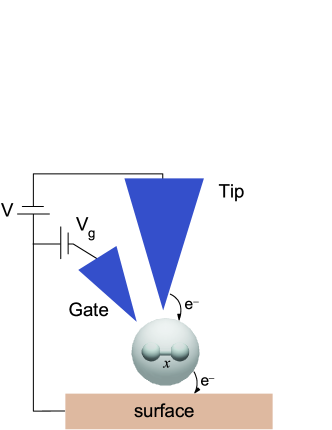
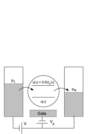
Figure 1: Upper part: Possible experimental setup. The STM tip is positioned above a molecule (represented as a sphere). An electron coming from the tip onto the molecule then tunnel into the conducting surface. A gate electrode is used to tune the molecular energy level(s) and to control the current flow between the STM tip and the conducting surface. Lower part: Schematic illustration of the model. By varying the gate voltage the molecular energy level can be shifted near the chemical potential of the electrodes. The molecular orbital energy $\varepsilon(x)$ and electron-electron interaction energy $U_{\mathrm{C}}(x)$ depend on the bond length $x$.

The complete Hamiltonian of the molecular junction consists of the molecular Hamiltonian (1), the Hamiltonians for noninteracting left and right electrodes, and the molecule-electrode interaction:

$$H=H_{M}+\sum_{\sigma,k\in L,R}\varepsilon_{k}a^{\dagger}_{\sigma k}a_{\sigma k}+\sum_{\sigma,k\in L,R}(t_{k}a^{\dagger}_{\sigma k}a_{\sigma}+\mbox{h.c.}),$$ (2)

where $a^{\dagger}_{\sigma k}$($a_{\sigma k}$) creates (annihilates) an electron in the single-particle state $\sigma k$ of either the left ($L$) or the right ($R$) electrode. The electron creation and annihilation operators satisfy standard fermionic anticommutation relations. The electron occupation numbers in both electrodes obey the Fermi-Dirac distribution $f_{L,R}(\varepsilon_{k})=[1+e^{(\varepsilon_{k}-\mu_{L,R})/T}]^{-1}$. The chemical potentials in the electrodes, $\mu_{L}$ and $\mu_{R}$, are assumed to be biased by the external symmetrically applied voltage $V=\mu_{L}-\mu_{R}$, which we take to be positive, and $\mu_{L,R}=\pm 0.5V$. The Fermi energies of the electrodes are set to zero. We also assume that the tunnelling matrix element $t_{k}$ is spin independent.

The coupling with the electrodes broadens the molecular level, with the width given by the imaginary part of the electrode self-energy,

$$\Gamma(\omega)=\Gamma_{L}+\Gamma_{R}=-\mathrm{Im}\sum\limits_{k\in L,R}|t_{k}|^{2}/(\omega-\varepsilon_{k}+i0^{+}).$$ (3)

In what follows, for the sake of simplicity, we will use the wide-band approximation for the electrodes, i.e., the imaginary part $\Gamma$ of the self-energy is energy independent and the real part vanishes. The total width of the molecular level is fixed in our numerical calculations, $\Gamma=1.36$ eV, but we vary the relative contributions of left and right electrodes.

We neglect the effect of the electric field on the molecule – for diatomic molecules lying flat on the metal surface the electric field is perpendicular to the bond length and does not influence the dynamics. In other cases, the electric field may give an additive contribution which can be easily included into the model for particular molecule-electrode geometries and inter-electrode distances.

We begin with the Ehrenfest coupled electron-nuclei dynamical equations

$$i\hbar\dot{\rho}(x,t)=[H,\rho(x,t)]$$ (4)

$$m\ddot{x}=-\mathrm{Tr}\bigl{[}\rho(x,t)\frac{\partial H}{\partial x}\bigr{]}.$$ (5)

We eliminate the electronic density matrix from this equation assuming that the electronic degrees of freedom vary much faster than the nuclear motion. Physically this means that the oscillation period $\tau_{p}$ of the reaction coordinate is much larger than the tunneling time for the electrons, i.e., $\tau_{p}\gg 1/\Gamma$. Below we will see that this assumption is fulfilled for the model under consideration. This eliminates the direct time dependence from the electronic density matrix $\rho(x,t)\sim\rho(x)$, which now depends parametrically on time through the reaction coordinate. The result is the following Langevin equation for the reaction coordinate,

$$m\ddot{x}=-\mathrm{Tr}\bigl{[}\rho(x)\frac{\partial H}{\partial x}\bigr{]}-\xi(x)\dot{x}+\delta f(x,t).$$ (6)

Here $\rho(x)$ is the nonequilibrium density matrix, $\xi(x)$ is the frictional force (viscosity), and $\delta f(x,t)$ is the random force (noise) taken in the Gaussian form

$$\langle\delta f(x,t)\rangle=0,~{}~{}~{}~{}\langle\delta f(x,t)\delta f(x,t^{\prime})\rangle=D(x)\delta(t-t^{\prime}),$$ (7)

The derivation of the Langevin equation via Keldysh nonequilibrium Green’s functions (NEGF) is presented in Appendix B.

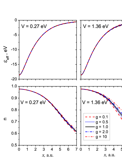
Figure 2: Effective single particle energy level $\varepsilon_{\mathrm{eff}}(x)$ and population $n(x)$ as a function of the reaction coordinate $x$ for different values of the asymmetry coefficient $g=\Gamma_{L}/\Gamma_{R}$ and applied voltage $V$. We chose $\varepsilon_{\mathrm{eff}}(x_{\mathrm{min}})=-9.8$ eV, where $x_{\mathrm{min}}=1.66$ a.u. corresponds to the minimum of the equilibrium potential energy of the molecule. The Fermi energies of the electrodes are set to zero.

To obtain expressions for the frictional force and noise intensity $D(x)$ we apply the mean-field approximation to the Hamiltonian (1), i.e., we replace it by

$$H^{\mathrm{mf}}_{M}=\varepsilon_{\mathrm{eff}}(x)\sum_{\sigma}n_{\sigma}+V_{N}(x)+\frac{p^{2}}{2m},$$ (8)

where

$$\varepsilon_{\mathrm{eff}}(x)=\varepsilon(x)+V_{g}+\frac{1}{2}U_{\mathrm{C}}(x)n(x)$$ (9)

is the effective single particle energy and $n(x)=\mathrm{Tr}[\rho(x)n_{\sigma}]$ is the nonequilibrium population of the electronic level of the molecule. This can be computed by means of the NEGF, see Eq. (50) in Appendix B. In Appendix B we also present the details of the derivation of the explicit expressions for $\xi(x)$ and $D(x)$.

For low temperatures, $T\to 0$, the Fermi-Dirac electron distributions in the electrodes $f_{L,R}(\omega)$ can be approximated by a step like function, and the level population, friction coefficient, and noise intensity can be written as

$$n(x)=\frac{1}{2}-\frac{1}{\pi\Gamma}\left\{\Gamma_{L}\arctan\left(\frac{\varepsilon_{\mathrm{eff}}(x)-\mu_{L}}{\Gamma}\right)\right.$$

$$+\left.\Gamma_{R}\arctan\left(\frac{\varepsilon_{\mathrm{eff}}(x)-\mu_{R}}{\Gamma}\right)\right\}$$ (10)

$$\xi(x)=\frac{2\Gamma}{\pi}\left\{\Gamma_{L}Q(\mu_{L},x)+\Gamma_{R}Q(\mu_{R},x)\right\},$$ (11)

$$D(x)=\frac{4\Gamma_{L}\Gamma_{R}}{\pi}\int_{\mu_{R}}^{\mu_{L}}d\omega\,Q(\omega,x),$$ (12)

where the function $Q(\omega,x)$ is defined as

$$Q(\omega,x)=\left[\frac{\varepsilon^{\prime}_{\mathrm{eff}}(x)}{(\omega-\varepsilon_{\mathrm{eff}}(x))^{2}+\Gamma^{2}}\right]^{2}.$$ (13)

Note that in the derivation of Eq. (11) we have utilized $(-\partial_{\omega}f_{\alpha})=f_{\alpha}(1-f_{\alpha})/T$ and $\lim\limits_{T\to 0}(-\partial_{\omega}f_{\alpha})=\delta(\omega-\mu_{\alpha})$.

Equations (9, 11, 12, II) are the main equations of our model. Their solution provides us with the parameters of the Langevin equation (6). Note that $\varepsilon_{\mathrm{eff}}(x)$ in (II) itself depends on $n(x)$, through Eq. (9). Therefore, both equations should be solved self-consistently. The main variables in our model are the applied voltage $V$ and the asymmetry coefficient $g=\Gamma_{L}/\Gamma_{R}$. The asymmetry coefficient $g$ controls the relative strength of the coupling to left and right electrodes. Replacing $g$ by $1/g$ is equivalent to reversing the applied voltage.

In Fig. 2 the effective single particle energy $\varepsilon_{\mathrm{eff}}(x)$ and the population $n(x)$ are depicted for two values of the applied voltage, small ($V=0.27$ eV) and large ($V=1.36$ eV), and for different values of the asymmetry coefficient $g$. The reference point for the effective molecular orbital energy is chosen to be $\varepsilon_{\mathrm{eff}}(x_{\mathrm{min}})=-9.8$ eV (relative to the electrode Fermi energy), where $x_{\mathrm{min}}=1.66$ a.u. determines the minimum of the $H_{2}$ ground state energy [see Eq.(32)]. This reference point can be shifted by the real part of the electrode self-energy, if we revoke the wide-band approximation, or by the application of a gate voltage $V_{g}$. The dependence of the results on gate voltage will be discussed below. As seen from the figure, at small values of the reaction coordinate, i.e., when the electron level is well below the electrode Fermi levels, both $\varepsilon_{\mathrm{eff}}(x)$ and $n(x)$ are nearly independent of the applied voltage and the asymmetry coefficient. The situation changes with increasing $x$, i.e., when $\varepsilon_{\mathrm{eff}}(x)$ comes into resonance with the electrode Fermi levels. In that case, the electron population is strongly affected by the asymmetry coefficient and the effect becomes more pronounced at larger values of $V$. As a result, at large $x$ and $V$ the effective single particle energy $\varepsilon_{\mathrm{eff}}(x)$ grows with increasing $g$.

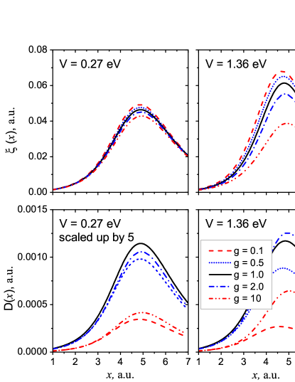
Figure 3: Friction coefficient $\xi(x)$ and noise intensity $D(x)$ as a function of the reaction coordinate $x$. All the parameters are the same as those in Fig. 2.

In Fig. 3 the friction coefficient $\xi(x)$ and the noise intensity $D(x)$ are plotted for the same parameters as those in Fig. 2. The friction coefficient grows with increasing $x$ and reaches its maximum value when $\varepsilon_{\mathrm{eff}}(x)$ is close to the chemical potentials of the electrodes, i.e., when the resonant regime is approached. The friction $\xi(x)$ becomes smaller when the molecule starts to fall apart (due to the decrease of $\varepsilon^{\prime}_{\mathrm{eff}}(x)$). As seen from the figure, the friction coefficient grows as the asymmetry coefficient is reduced and this dependence is more pronounced for larger values of $V$. Besides, for small values of $g$ the friction is more sensitive to changes in the applied voltage.

The noise intensity $D(x)$ also reaches its maximum value when $\varepsilon_{\mathrm{eff}}(x)$ is close to the chemical potentials of the electrodes. However, in contrast to the previous case, $D(x)$ is maximal for symmetric coupling to the electrodes, i.e., when $g=1$. Moreover, because of the integral in Eq. (12) the order of magnitude of $D(x)$ is proportional to the applied voltage.

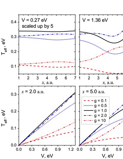
Figure 4: Upper panels: Effective temperature $T_{\mathrm{eff}}$ as a function of the reaction coordinate $x$ for two values of the applied voltage $x$. Lower panels: Effective temperature $T_{\mathrm{eff}}$ as a function of the applied voltage $V$ for two values of the reaction coordinate $x$. All the parameters are the same as those in Fig. 2.

Motivated by the fluctuation-dissipation theorem, we can also introduce an effective ”temperature” which depends on the reaction coordinate,

$$T_{\mathrm{eff}}(x)=\frac{D(x)}{2\xi(x)}=\frac{\Gamma^{-1}\Gamma_{R}\Gamma_{L}\int_{\mu_{R}}^{\mu_{L}}Q(\omega,x)d\omega}{\Gamma_{L}Q(\mu_{L},x)+\Gamma_{R}Q(\mu_{R},x)}.$$ (14)

Assuming that $Q(\omega,x)\approx\mathrm{const}$ for $\mu_{L}>\omega>\mu_{R}$ we can approximate (14) by

$$T_{\mathrm{eff}}(x)\approx T(V,g)=V\frac{\Gamma_{R}\Gamma_{L}}{\Gamma^{2}}=V\frac{g}{(1+g)^{2}},$$ (15)

The effective temperature (15) has a maximum of $V/4$ when $g=1$. Note that the current is also maximal when the coupling to the electrodes is symmetric. In the upper panels of Fig. 4 the effective temperature $T_{\mathrm{eff}}(x)$ is shown for the same parameters as those in Fig. 2 for two values of the applied voltage. As seen, for small applied voltages $T_{\mathrm{eff}}(x)$ is nearly independent of $x$ and can be approximated by Eq. (15). When the applied voltage increases the effective temperature also grows and $T_{\mathrm{eff}}$ becomes dependent on the reaction coordinate in a rather nontrivial way. The lower panels of Fig. 4 depict the effective temperature as a function of $V$ for two particular values of the reaction coordinate. The point $x=2.0$ a.u. is close to the minimum of the effective potential, while $x=5.0$ a.u. is near the top of the barrier. We emphasize that by reversing the applied voltage polarity (i.e., replacing $g$ by $1/g$) we can vary the effective temperature and the effect is more pronounced the larger the value of $V$.

III Reaction rates

III.1 Fokker-Planck equation for the reaction coordinate

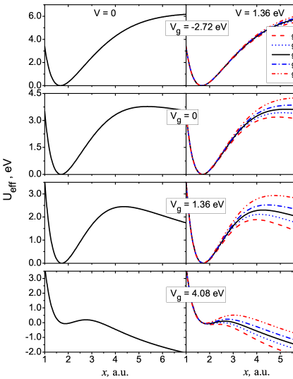
Figure 5: Effective nonequilibrium potential $U_{\mathrm{eff}}(x)$ as a function of the reaction coordinate $x$ for two values of the applied voltage $V$. The panels correspond to different positions of the effective molecular orbital energy relative to the electrode Fermi energy $\varepsilon_{\mathrm{eff}}(x_{\mathrm{min}})=-9.8\mbox{ eV}+V_{g}$. All other parameters are the same as those in Fig. 2.

Since $\partial H/\partial x=\varepsilon^{\prime}_{\mathrm{eff}}(x)\sum_{\sigma}n_{\sigma}+V^{\prime}_{N}(x)$ in mean-field approximation, Eq. (6) becomes

$$m\ddot{x}=-2\varepsilon^{\prime}_{\mathrm{eff}}(x)n(x)-V^{\prime}_{N}(x)-\xi(x)\dot{x}+\delta f(x,t).$$ (16)

The Langevin equation (16) is equivalent to the Fokker-Planck equation for the distribution function $F(x,p,t)$,

$$\frac{\partial}{\partial t}F=-\left\{U^{\prime}_{\mathrm{eff}}(x)\frac{\partial}{\partial p}-\frac{p}{m}\frac{\partial}{\partial x}\right\}F$$

$$+\frac{\xi(x)}{m}\frac{\partial}{\partial p}(pF)+\frac{D(x)}{2}\frac{\partial^{2}}{\partial p^{2}}F.$$ (17)

Here the effective nonequilibrium potential energy surface is defined via integration of the nonequilibrium force in the Langevin equation,

$$U_{\mathrm{eff}}(x)=V_{N}(x)+2\int_{x_{0}}^{x}\varepsilon^{\prime}_{\mathrm{eff}}(y)n(y)dy.$$ (18)

In Fig. 5 the nonequilibrium effective potential is shown as a function of the reaction coordinate for different values of the asymmetry coefficient $g$, applied voltage bias $V$, and gate voltage $V_{g}$. The current flow through the molecule changes the height of the potential barrier: for $g<1$ the current reduces the barrier height and for $g>1$ the current increases it. The explanation is the following: when the coupling to the left electrode is stronger ($g>1$) the current pumps electrons into the molecule and enhances the chemical bond. Conversely, when the coupling to the right electrode is stronger the current depletes the molecular electrons, thereby weakening the chemical bond. Thus, by reversing the voltage polarity we can vary the height of the potential barrier. But it should be stressed that the effective temperature $T_{\mathrm{eff}}$ also changes with reversing the voltage polarity and the barrier growth is accompanied by a temperature increase. We also see from Fig. 5 that the height of the potential barrier can be decreased by increasing the gate voltage. The resonant tunneling regime $V_{g}=0$ and $V_{g}=1.36$ eV is physically most interesting, since the nonequilibrium potential energy profile exhibits a clear barrier between product and reactant states. We focus on the resonant tunnelling regime in our calculations of the reaction rates.

	$V_{g}=0.0$				$V_{g}=1.36$ eV
$k$	$g=0.1$	$g=1.0$	$g=10$		$g=0.1$	$g=1.0$	$g=10$
$0.1$	400	405	393		435	414	407
$0.5$	498	496	497		515	500	491
$0.9$	781	806	817		744	752	776

Table 1: The period of motion (Eq. (19), a.u. of time) in the nonequilibrium effective potential (the bias voltage $V=1.36$ eV) for different values of the asymmetry coefficient $g$ and the gate voltage $V_{g}$. The parameter $k$ defines the energy, $k=(E-E_{\mathrm{min}})/(E_{\mathrm{max}}-E_{\mathrm{min}})$. All other parameters are the same as those in Fig. 2.

Now we want to reduce the Fokker-Planck equation (III.1) to the Smoluchowski equation for the distribution function which depends either on the reaction coordinate $x$ (overdamped motion) or on the energy $E=\frac{p^{2}}{2m}+U_{\mathrm{eff}}(x)$ (underdamped motion). To find which case is realized for the considered model we compare the oscillation period along the reaction coordinate and the relaxation time due to friction. The oscillation period is given by

$$\tau_{p}(E)=2\int_{x_{1}}^{x_{2}}\frac{dx}{\dot{x}}=2\int_{x_{1}}^{x_{2}}\frac{dx}{\sqrt{\frac{2}{m}(E-U_{\mathrm{eff}}(x))}},$$ (19)

where $x_{1}$ and $x_{2}$ are left and right turning points, i.e., $E=U_{\mathrm{eff}}(x_{1,2})$. If $E\approx U_{\mathrm{eff}}(x_{\mathrm{min}})$ then $\tau_{p}\approx 2\pi/\omega_{0}$, where $\omega_{0}=\sqrt{U^{\prime\prime}_{\mathrm{eff}}(x_{\mathrm{min}})/m}$ is the oscillation frequency near the bottom of the effective potential. In Table 1 the oscillation period is computed for various values of the bias voltage, gate voltage, and asymmetry coefficient. Since $\tau_{p}\gg 1/\Gamma$ ($\Gamma=0.05$ a.u.) the assumption behind the derivation of the Langevin equation (appendix B), namely the assumption that the electronic degrees of freedom are much faster than the motion along $x$ is fulfilled. In Fig. 3 the friction $\xi(x)$ is shown for different values of asymmetry coefficient $g$ and applied voltage $V$. It is evident that the relaxation time due to the friction $m/\xi(x)$ is much larger than the oscillation period. Therefore the energy dissipation per period of the motion is small, which means that we deal with underdamped motion.

III.2 Calculations of the reaction rates

The solution of the Fokker-Planck equation is not trivial in our case, since the effective temperature depends on the reaction coordinate. Using the method described by Coffey et al. Coffey et al. (1996) the Fokker-Planck equation is reduced to the equation for the distribution function for the energy, $P(E,t)$

$$\frac{\partial}{\partial t}P(E,t)= \frac{\partial}{\partial E}\left[\xi(E)P(E,t)\right]$$

$$+\frac{1}{2}\frac{\partial}{\partial E}\left[D(E)\frac{\partial}{\partial E}P(E,T)\right],$$ (20)

where

$$\xi(E)=\frac{1}{T(E)}\int_{x_{1}}^{x_{2}}\xi(x)\dot{x}dx$$ (21)

and

$$D(E)=\frac{1}{T(E)}\int_{x_{1}}^{x_{2}}D(x)\dot{x}dx.$$ (22)

By introducing

$$\alpha(E)=\frac{1}{2}\frac{\partial}{\partial E}D(E)-\xi(E)$$ (23)

we re-write this equation as the Smoluchowski equation

$$\frac{\partial}{\partial t}P(E,t)=-\frac{\partial}{\partial E}\left[\alpha(E)P(E,t)\right]+\frac{1}{2}\frac{\partial^{2}}{\partial E^{2}}\left[D(E)P(E,T)\right].$$ (24)

The same equation was obtained in Ref. Mozyrsky et al., 2006, though the theory was applied only to a nano-mechanical harmonic oscillator and thus did not consider dissociation processes. Then, the mean time for a particle with initial energy $E_{\mathrm{min}}=U_{\mathrm{eff}}(x_{\mathrm{min}})$ to arrive at the top $E_{\mathrm{max}}=U_{\mathrm{eff}}(x_{\mathrm{max}})$ of the potential barrier is given by (see, for example, Eq. XII.3.7 in Ref. Van Kampen, 2007)

$$\tau=2\int_{E_{\mathrm{min}}}^{E_{\mathrm{max}}}dEe^{\Phi(E)}\int^{E}_{E_{\mathrm{min}}}\frac{dE^{\prime}}{D(E^{\prime})}e^{-\Phi(E^{\prime})},$$ (25)

where

$$\Phi(E)=-\int_{E_{0}}^{E}\frac{2\alpha(E^{\prime})}{D(E^{\prime})}dE^{\prime}.$$ (26)

Note, that the choice of $E_{0}$ is not relevant since it does not contribute to the escape time (25). Using relation (23) we can rewrite (25) as

$$\tau=2\int_{E_{\mathrm{min}}}^{E_{\mathrm{max}}}\frac{dE}{D(E)}e^{\Psi(E)}\int^{E}_{E_{\mathrm{min}}}e^{-\Psi(E^{\prime})}dE^{\prime},$$ (27)

where

$$\Psi(E)=\int_{E_{0}}^{E}\frac{1}{T_{\mathrm{eff}}(E^{\prime})}dE^{\prime}$$ (28)

in terms of the effective temperature $T_{\mathrm{eff}}(E)={D(E)}/2\xi(E)$.

Equation (27) gives us the exact escape time (mean first passage time) for the Brownian particle in the underdamped regime with coordinate-dependent effective temperature. In our particular case it can be further simplified, because our calculations show that the effective temperature $T_{\mathrm{eff}}(E)$ depends only slightly on energy when $E_{\mathrm{min}}<E<E_{\mathrm{max}}$ and can be approximated by Eq. (15)., i.e., $T_{\mathrm{eff}}(E)=T(V,g)$. With this approximation, the integral (28) becomes $\Psi(E)\approx E/T_{\mathrm{eff}}(E)$. Substituting this into Eq. (27) we obtain

$$\tau\approx 2T_{\mathrm{eff}}(E_{\mathrm{min}})\int_{E_{\mathrm{min}}}^{E_{\mathrm{max}}}\frac{dE}{D(E)}\exp\left\{\frac{E-E_{\mathrm{min}}}{T_{\mathrm{eff}}(E)}\right\},$$ (29)

This formula gives us the escape time from the nonequilibrium potential barrier with the effective temperature which depends on the energy of the particle.

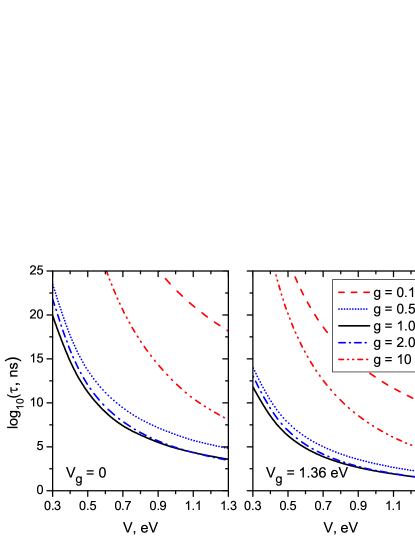
Figure 6: Escape time computed for various values of the asymmetry coefficient $g$ as a function of the applied voltage. The left and right panels correspond to different positions of the effective molecular orbital energy relative to the electrode Fermi energy $\varepsilon_{\mathrm{eff}}(x_{\mathrm{min}})=-9.8\mbox{ eV}+V_{g}$. All other parameters are the same as those in Fig. 2.

In Fig. 6 we show the escape time (29) computed for various values of the asymmetry coefficient $g$ as a function of the applied voltage $V$. For all values of $g$ the escape time decreases with increasing applied voltage. We also see that moving the molecular orbital closer to the Fermi energy of the electrodes facilitates the dissociation. When the noise is balanced by the viscosity, i.e. when the fluctuation-dissipation relations is forced for the nuclear degrees of freedom,Dzhioev and Kosov (2011) the dependence of the reaction rates on asymmetry coefficient is more complicated. For example, it was shown that the chemical reaction can be catalysed or stopped depending on the direction of the electric current.Dzhioev and Kosov (2011) In contrast, the absence of the fluctuation-dissipation relation leads to a rise of the effective temperature $T_{\mathrm{eff}}(x)$ (or $T_{\mathrm{eff}}(E)$) which always overrides the increase of the nonequilibrium potential barrier. We also see from the figure that for asymmetric coupling the escape time can be controlled by changing the applied voltage polarity, i.e., by replacing $g$ by $1/g$.

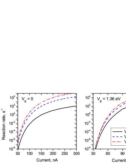
Figure 7: Reaction rate for the molecule dissociation computed at the fixed applied voltage as a function of the electric current. The left and right panels correspond to different positions of the effective molecular orbital energy relative to the electrode Fermi energy $\varepsilon_{\mathrm{eff}}(x_{\mathrm{min}})=-9.8\mbox{ eV}+V_{g}$. In our calculations we choose the right coupling fixed, $\Gamma_{R}=1.36$ eV, and vary the left coupling to change the current at constant applied voltage. All other parameters are the same as those in Fig. 2.

In experiments on STM induced molecular dissociation, the applied voltage bias is usually fixed while the electric current is varied by changing the distance between STM tip and molecule.Stipe et al. (1997) In the following, we apply our approach to model this experimental scenario. Similar to the experimental conditions, we keep the coupling to the surface, $\Gamma_{R}$, and the applied bias voltage fixed. Then we compute the reaction rate (inverse escape time) as a function of the electric current by changing the coupling to the left electrode $\Gamma_{L}$, which is equivalent to changing the distance between STM tip and molecule. The results of the calculation are shown in Fig.7. Our calculations predict a rather nontrivial dependence of the reaction rate on the tunnelling current. Note that these results reveal much more structure than the power law dependence on current reported experimentally for a related but different system, namely O₂.Stipe et al. (1997) The main reason for this is the following. The simple estimation shows that the coupling to the STM tip, $\Gamma_{L}$, which reflects the experimental conditions,Stipe et al. (1997) is of order $0.001$ eV. This makes the electronic tunneling rate small compared to the vibrational frequency of the molecule. In this limit, a simple Fermi Golden Rule calculation applies and gives a power law dependence of the reaction rate.Stipe et al. (1997) In contrast, we treat the interesting limit of larger electronic currents where the molecule is in fully developed nonequilibrium. It is in this regime that we predict a highly nontrivial current dependence of the dissociation rate. This reflects the fact that our approach is geared towards fully developed nonequilibrium, while previous work effectively treated systems close to thermal equilibrium. Therefore, the absence of a simple power low dependence of the reaction rate and the appearance of nontrivial nonlinear behaviour as shown in Fig.7 may serve as an indication of fully developed electronic nonequilibrium.

IV Conclusions

In this paper, we have formulated and solved Kramers problem for current-induced, out of equilibrium chemical reactions. As a general model of covalent bond breaking, we have considered the dissociation of a diatomic molecules induced by the tunnelling current from a STM tip. We have proposed a model Hamiltonian for the system and, by projecting out the electronic degrees of freedom, we have derived a Langevin equation for the time evolution of the reaction coordinate. The Langevin equation leads to Fokker-Planck dynamics with an effective temperature which depends on the reaction coordinate. The reaction rate for the dissociation is computed by solving the Fokker-Planck equation for the escape time. In the resonant tunnelling regime, two processes play equally important roles in the molecular dissociation: the decrease of the potential energy barrier and reaction-coordinate-dependent local heating of the molecule. The current induced catalytic reduction of the barrier accompanied by the local heating is an alternative mechanism for current-induced bond breaking, which is very different from the widely accepted paradigm of merely pumping vibrational degrees of freedom.

Appendix A Parametrization of the Hamiltonian

In our calculations we take $\varepsilon(x)$ in the form of the bonding orbital for the $H_{2}^{+}$ molecule in the gas phase McQuarrie (2007)

$$\varepsilon(x)=-\frac{1}{2}+\frac{J(x)+K(x)}{1+S(x)}$$ (30)

where the functions $J(x),~{}K(x),~{}S(x)$ are given by

$$J(x) =\mathrm{e}^{-2x}\left(1+\frac{1}{x}\right)-\frac{1}{x},~{}~{}K(x)=-\mathrm{e}^{-x}(1+x),$$

$$S(x) =\mathrm{e}^{-x}\left(1+x+\frac{x^{2}}{3}\right).$$ (31)

The Coulomb interaction between electrons $U_{\mathrm{C}}(x)$ is chosen such to reproduce, within the equilibrium ($n(x)=1,~{}V_{g}=0$) mean-field Hamiltonian (2), the energy of the $H_{2}$ molecule obtained within the molecular orbital theory (see Appendix on page 543 in Ref. McQuarrie, 2007), i.e.,

$$\langle{H^{\mathrm{mf}}_{M}}\rangle=E_{MO}(x)=2\varepsilon(x)+U_{\mathrm{C}}(x)+\frac{1}{x}.$$ (32)

Here we neglect the nuclear kinetic energy contribution. Therefore, $U_{\mathrm{C}}(x)$ can be written as follows

$$U_{\mathrm{C}}(x)=\frac{\frac{5}{16}+0.5J_{p}(x)+K_{p}(x)+2L(x)}{(1+S(x))^{2}},$$ (33)

where the functions $L(x),~{}J_{p}(x),~{}K_{p}(x)$ are listed in Table 10.8 of Ref. McQuarrie, 2007.

Appendix B Derivation of the Langevin equation for the reaction coordinate via NEGF

The Langevin equation for nuclear degrees of freedom coupled to out-of-equilibrium electrons has recently been given in various contexts Mozyrsky et al. (2006); Pistolesi et al. (2008); Bode et al. (2011, 2012); Lü et al. (2012); Thomas et al. (2012). To make this paper self-contained, we provide here an explicit derivation which is directly adapted to the Hamiltonian under consideration. Our starting point is the Heisenberg equation of motion for the reaction coordinate as obtained from the mean-field Hamiltonian (2),

$$m\ddot{x}+\frac{\partial V_{N}}{\partial x}=-\varepsilon^{\prime}_{\rm eff}(x)\sum_{\sigma}a^{\dagger}_{\sigma}a_{\sigma}\,,$$ (34)

Here, the right-hand side contains the operator describing the current-induced forces. Given that the molecular dissociation dynamics is slow compared to the electronic degrees of freedom, we calculate these forces within a nonequilibrium adiabatic approximation. In this approximation, the reaction coordinate is taken as classical. The electronic state should be computed for a given trajectory $x=x(t)$ while in turn, the electrons affect this trajectory through adiabatic reaction forces.

In the nonequilibrium adiabatic approximation, one averages the force appearing on the right-hand side of Eq. (34) over times which are long on the scale of the electronic dynamics, but short on the scale of the dissociation dynamics. The average adiabatic reaction force is thus given by the expectation value $\langle\varepsilon^{\prime}_{\rm eff}(x)a_{\sigma}^{\dagger}a_{\sigma}\rangle_{x(t)}$, evaluated for a given trajectory ${x}(t)$ of the reaction coordinate. The fluctuation-dissipation theorem implies that we need to include a fluctuating Langevin force $\delta f(t)$ in addition to the friction force. Hence Eq. (34) becomes

$$m\ddot{x}+\frac{\partial V_{N}}{\partial x}=2i\varepsilon^{\prime}_{\rm eff}(x){\cal G}^{<}(t,t)+\delta f(t),$$ (35)

where we have introduced the lesser Green’s function

$${\cal G}^{<}(t,t^{\prime})=i\langle a_{\sigma}^{\dagger}(t^{\prime})a_{\sigma}(t)\rangle_{{x}(t)}\,,$$ (36)

and the factor of two accounts for spin. Thus, except for the stochastic noise force, the current-induced forces are encoded in $2i\varepsilon^{\prime}_{\rm eff}(x){\cal G}^{<}$. Below we demonstrate that the current-induced forces can be represented as a sum of two contributions: the adiabatic force and a velocity-dependent contribution,

$$2i\varepsilon^{\prime}_{\rm eff}(x){\cal G}^{<}\simeq F(x)-\xi(x)\dot{x}.$$ (37)

The variance of the stochastic force $\delta f(t)$ is governed by the symmetrized fluctuations of the operator $\varepsilon^{\prime}_{\rm eff}(x)a_{\sigma}^{\dagger}a_{\sigma}$. Given that the electronic fluctuations happen on short time scales, $\delta f(t)$ is locally correlated in time,

$$\langle\delta f(t)\delta f(t^{\prime})\rangle=D({x})\delta(t-t^{\prime})\,.$$ (38)

Since we are dealing with a mean-field Hamiltonian, $D({x})$ can be evaluated using Wick’s theorem,

$$\langle\delta f(t)\delta f(t^{\prime})\rangle=2[\varepsilon^{\prime}_{\rm eff}(x)]^{2}{\cal G}^{>}(t,t^{\prime}){\cal G}^{<}(t^{\prime},t)\,,$$ (39)

where

$${\cal G}^{>}(t,t^{\prime})=-i\langle a_{\sigma}(t)a_{\sigma}^{\dagger}(t^{\prime})\rangle_{{x}(t)}\,$$ (40)

is the greater Green’s function. These expressions show that we need to evaluate the electronic Green’s function for a given classical trajectory ${x}(t)$.

We start with the Keldysh equation for lesser Green’s function:

$${\cal G}^{<}(t,t^{\prime})=\int\mathrm{d}t_{1}\int\mathrm{d}t_{2}\,{\cal G}^{R}(t,t_{1})\Sigma^{<}(t_{1},t_{2}){\cal G}^{A}(t_{2},t^{\prime})\,,$$ (41)

where the retarded and advanced Green’s functions are given by the standard expressions

$${\cal G}^{R}(t,t^{\prime})=-i\theta(t-t^{\prime})\langle\{a_{\sigma}(t),a_{\sigma}^{\dagger}(t^{\prime})\}\rangle_{{x}(t)}\,,$$ (42)

$${\cal G}^{A}(t,t^{\prime})={\cal G}^{R}(t^{\prime},t)^{*}.$$ (43)

The Keldysh equation (41) involves the lesser self-energy

$$\Sigma^{<}(\omega)=2i\,\sum_{\alpha}f_{\alpha}(\omega)\Gamma_{\alpha}(\omega)\,,$$ (44)

where $f_{\alpha}(\omega)=[1+e^{\beta_{\alpha}(\omega-\mu_{\alpha})}]^{-1}$ is the Fermi-Dirac electron distribution in the left ($\alpha=L$) or the right ($\alpha=R$) electrode, and $\Gamma_{\alpha}(\omega)$ is the imaginary part of the retarded self-energy due to interaction with the electrodes

$$\Sigma^{R}_{\alpha}(\omega)=\sum\limits_{k\in\alpha}\frac{|t_{k}|^{2}}{\omega-\varepsilon_{k}+i0^{+}}=\Lambda_{\alpha}(\omega)-i\Gamma_{\alpha}(\omega).$$ (45)

The adiabatic expansion of Keldysh equation is carried out in the Wigner representation, given by

$$\tilde{A}(t,\omega)=\int\mathrm{d}\tau\,e^{i\omega\tau}A(t+\tau/2,t-\tau/2)$$ (46)

for a general function $A(t,t^{\prime})$, in which fast and slow time scales are easily identifiable. For the Green’s function ${\cal G}^{A,R,<}$, the slow mechanical motion implies that ${\cal G}^{A,R,<}(t_{1},t_{2})$ varies slowly with the central time $t=\frac{t_{1}+t_{2}}{2}$, but oscillates fast with the relative time $\tau=t_{1}-t_{2}$. As usual, the Wigner transform of a convolution $C(t_{1},t_{2})=\int\mathrm{d}t_{3}\,A(t_{1},t_{3})B(t_{3},t_{2})$ is given by

$$\tilde{C} = \exp\left[\frac{i}{2}\left(\partial_{\epsilon}^{\tilde{A}}\partial_{t}^{\tilde{B}}-\partial_{t}^{\tilde{A}}\partial_{\epsilon}^{\tilde{B}}\right)\right]\tilde{A}\tilde{B}$$ (47)

$$\simeq \tilde{A}\tilde{B}+\frac{i}{2}\partial_{\epsilon}\tilde{A}\partial_{t}\tilde{B}-\frac{i}{2}\partial_{t}\tilde{A}\partial_{\epsilon}\tilde{B},$$

where we have dropped higher order derivatives in the last line, exploiting the slow variation with the central time $t$.

Expanding Eq. (41) up to the leading adiabatic correction according to Eq. (47) and taking into account that $\Sigma^{<}$ depends only on $\omega$ and is independent of the central time, we obtain ${\cal G}^{<}$ to first order in $\dot{x}$,

$${\cal\tilde{G}}^{<}= G^{<}+\frac{i}{2}\,\dot{x}\,\varepsilon^{\prime}_{\rm eff}(x)\,\left[G^{<}\partial_{\omega}G^{>}+G^{>}\partial_{\omega}G^{<}\right]$$ (48)

Here ${\cal\tilde{G}}$ denotes full Green’s functions in Wigner representation, while $G$ denotes the strictly adiabatic (or ”frozen”) Green’s functions that are evaluated for a fixed value of $x$: $G^{R}(x,\omega)=\left[\omega-\varepsilon_{{\rm eff}}(x)-\Sigma^{R}(\omega)\right]^{-1}$, $\Sigma^{R}(\omega)=\sum_{\alpha}\Sigma^{R}_{\alpha}(\omega)$, ${G}^{A}=({G}^{R})^{\dagger}$, $G^{<}=G^{R}\Sigma^{<}G^{A}$, $G^{>}=G^{<}+G^{R}-G^{A}$.

Let us now compute the current-induced forces appearing in the Langevin equation (6). In the strictly adiabatic limit, i.e., retaining only the first term on the RHS of Eq. (48), ${\cal\tilde{G}}^{<}\simeq G^{<}$, we obtain the mean force

$$F(x)=-2\varepsilon^{\prime}_{\rm eff}(x)\,n(x)\,$$ (49)

where $n(x)$ is the nonequilibrium population of the electronic level

$$n(x)=\int\frac{d\omega}{2\pi i}\,G^{<}(x,\omega).$$ (50)

The leading order correction in Eq. (48) gives a velocity-dependent contribution to the current induced forces, which determines the friction $\xi(x)$ in the Langevin equation. After integration by parts we obtain the explicit expression

$$\xi(x)=2[\varepsilon^{\prime}_{\rm eff}(x)]^{2}\int\frac{d\omega}{2\pi}\,G^{<}(x,\omega)\partial_{\omega}G^{>}(x,\omega).$$ (51)

We evaluate the noise intensity $D(x)$ (39) for the stochastic force $\delta f$ to the lowest order in the adiabatic expansion, so that

$$D(x)=2[\varepsilon^{\prime}_{\rm eff}(x)]^{2}\int\frac{d\omega}{2\pi}\,{G}^{>}(x,\omega){G}^{<}(x,\omega).$$ (52)

Expressions Eqs, (51,52) can be simplified if we use the wide-band approximation for the electrodes. Namely, the wide-band limit employs that the retarded self-energy is energy independent, $\Sigma_{\alpha}^{R}(\omega)=-i\Gamma_{\alpha}$. In that case

$$G^{<}(x,\omega)=2i\frac{\sum_{\alpha}f_{\alpha}\Gamma_{\alpha}}{(\omega-\varepsilon_{\mathrm{eff}}(x))^{2}+\Gamma^{2}}$$ (53)

and we we obtain the following expressions for the friction

$$\xi(x)=4\Gamma\int\frac{d\omega}{2\pi}\,Q(\omega,x)\sum_{\alpha=L,R}(-\partial_{\omega}f_{\alpha})\Gamma_{\alpha}$$ (54)

and the noise intensity

$$D(x)=8\int\frac{d\omega}{2\pi}\,\,Q(\omega,x)\sum_{\alpha\alpha^{\prime}=L,R}\Gamma_{\alpha}\Gamma_{\alpha^{\prime}}f_{\alpha}(1-f_{\alpha^{\prime}}).$$ (55)

Here, the factor $Q(\omega,x)$ is given by Eq. (13).

References

- Stipe et al. (1997) B. C. Stipe, M. A. Rezaei, W. Ho, S. Gao, M. Persson, and B. I. Lundqvist, Phys. Rev. Lett. 78, 4410 (1997).
- Lauhon and Ho (2000) L. J. Lauhon and W. Ho, Phys. Rev. Lett. 84, 1527 (2000).
- Lee and Ho (1999) H. J. Lee and W. Ho, Science 286, 1719 (1999).
- Hla et al. (2000) S.-W. Hla, L. Bartels, G. Meyer, and K.-H. Rieder, Phys. Rev. Lett. 85, 2777 (2000).
- Repp et al. (2006) J. Repp, G. Meyer, S. Paavilainen, F. E. Olsson, and M. Persson, Science 312, 1196 (2006).
- Miller (1993) W. H. Miller, Acc. Chem. Res. 26, 174 (1993).
- Truhlar et al. (1983) D. G. Truhlar, W. L. Hase, and J. T. Hynes, J. Phys. Chem. 87, 2664 (1983).
- Manthe (2011) U. Manthe, Molecular Physics 109, 1415 (2011).
- Tully (1990) J. C. Tully, J. Chem. Phys. 93, 1061 (1990).
- Alavi et al. (1994) A. Alavi, J. Kohanoff, M. Parrinello, and D. Frenkel, Phys. Rev. Lett. 73, 2599 (1994).
- Doltsinis and Marx (2002) N. L. Doltsinis and D. Marx, Phys. Rev. Lett. 88, 166402 (2002).
- Head-Gordon and Tully (1995) M. Head-Gordon and J. C. Tully, J. Chem. Phys. 103, 10137 (1995).
- Dzhioev and Kosov (2011) A. A. Dzhioev and D. S. Kosov, J. Chem. Phys. 135, 074701 (2011).
- Koch et al. (2006) J. Koch, M. Semmelhack, F. von Oppen, and A. Nitzan, Phys. Rev. B 73, 155306 (2006).
- Härtle and Thoss (2011) R. Härtle and M. Thoss, Phys. Rev. B 83, 115414 (2011).
- Coffey et al. (1996) W. T. Coffey, Y. P. Kalmykov, and J. Waldron, The Langevin Equation: With Applications in Physics, Chemistry and Electrical Engineering (World Scientific, Singapore, 1996).
- Mozyrsky et al. (2006) D. Mozyrsky, M. B. Hastings, and I. Martin, Phys. Rev. B 73, 035104 (2006).
- Van Kampen (2007) N. G. Van Kampen, Stochastic Processes in Physics and Chemistry (3th ed. Elsevier, Amsterdam, 2007).
- McQuarrie (2007) D. A. McQuarrie, Quantum Chemistry (University Science Books, Sausalito, California, 2007).
- Pistolesi et al. (2008) F. Pistolesi, Y. M. Blanter, and I. Martin, Phys. Rev. B 78, 085127 (2008).
- Bode et al. (2011) N. Bode, S. V. Kusminskiy, R. Egger, and F. von Oppen, Phys. Rev. Lett. 107, 036804 (2011).
- Bode et al. (2012) N. Bode, S. V. Kusminskiy, R. Egger, and F. von Oppen, Beilstein J. Nanotechnol 3, 144 (2012).
- Lü et al. (2012) J.-T. Lü, M. Brandbyge, P. Hedegård, T. N. Todorov, and D. Dundas, Phys. Rev. B 85, 245444 (2012).
- Thomas et al. (2012) M. Thomas, T. Karzig, S. V. Kusminskiy, G. Zaránd, and F. von Oppen, Phys. Rev. B 86, 195419 (2012).