Optimal transport and von Neumann entropy in an Heisenberg XXZ chain out of equilibrium

Abstract

In this paper we investigate the spin currents and the von Neumann entropy (VNE) of an Heisenberg XXZ chain in contact with twisted XY-boundary magnetic reservoirs by means of the Lindblad master equation. Exact solutions for the stationary reduced density matrix are explicitly constructed for chains of small sizes by using a quantum symmetry operation of the system. These solutions are then used to investigate the optimal transport in the chain in terms of the VNE. As a result we show that the maximal spin current always occurs in the proximity of extrema of the VNE and for particular choices of parameters (coupling with reservoirs and anisotropy) it can exactly coincide with them. In the limit of strong coupling we show that minima of the VNE tend to zero, meaning that the maximal transport is achieved in this case with states that are very close to pure states.

I Introduction

There is presently an increasing amount of interest for the understanding of the transport properties in quantum open (out of equilibrium) systems Petruccione ; PlenioJumps due to possible application in the field of condensed matter physics and of quantum computing. In particular, transport properties in anisotropic XXZ Heisenberg spin chains in contact with magnetic reservoirs have been extensively investigated in the past years (for extended reviews see Ref. review1 ; zotos ) with a range of alternate methods, including exact diagonalizations zotos96 ; andrei98 , Bethe-ansatz shastry ; klumper ; zotos99 , Lagrange multipliers Anta97 ; Anta98 , Lanczos method lanczos , quantum Monte Carlo alvarez , etc. On the other hand, it is well known that these systems can be also treated by replacing observables associated with the reservoirs (or more in general with the environment) by means of quantum noise and studying the remaining degrees of freedoms within the formalism of the quantum open systems Petruccione . Within the Markovian approximation this amounts to model reservoirs by means of Lindblad operators acting at the system ends and to replace the Liouville equation for the time evolution of the density matrix with a master equation of Lindblad type for the reduced density matrix acting of the Hilbert space associated to the degrees of freedoms of physical interest Petruccione ; PlenioJumps .

The aim of the present paper is to use the formalism of the Lindblad master equation to provide a first characterization of the optimal transport in an open spin chain out of equilibrium in terms of the von Neumann entropy (VNE). In this respect we consider a XXZ Heisenberg chain with twisted XY boundary reservoirs at the ends which possesses inversion symmetry with respect to the middle point of the chain. By means of this symmetry we derive a set of algebraic equations which allow to compute in exact manner the stationary density matrix elements for chains of small sizes. As a result we show that the maximal spin current always occurs in proximity of a minimum of the VNE and for particular choices of parameters it can exactly coincide with it. We also show that in the strong coupling limit the minima of the VNE approach zero (exactly vanishing for infinite coupling), this meaning that the optimal transport is achieved in this case with states that are very close to pure states.

We remark that the open XXZ chain with an effective constant pumping at the chain ends which induce a gradient along the $z$ axis Casati2009 or with easy-plane magnetizations at the boundaries PSS2012 , have also been investigated. To the best of our knowledge, however, no specific link between optimal transport and extrema of VNE has been previously reported.

The paper is organized as follows. In Section II we present the model equation and discuss the quantum symmetry of the system. We show (in this section and in the Appendix) how the symmetry operator can be used to derive a set of algebraic equations which allow to obtain elements of the stationary reduced density matrix in exact manner. In Section III this approach is used to investigate the relationship between spin current and optimal transport in terms of the VNE for chains of small size. In the last Section the main results of the paper are briefly summarized.

II Model Equation and Symmetry Properties

We consider the quantum Master equation for the open XXZ model in the Lindblad form:

$$\frac{\partial\rho}{\partial t}=-i\left[H,\rho\right]+\gamma[-\frac{1}{2}\sum_{m}\left\{\rho,L_{m}^{{\dagger}}L_{m}\right\}+\sum_{m}L_{m}\rho L_{m}^{{\dagger}}]$$ (1)

where $\rho$ is the reduced density matrix, $H$ is the $XXZ$ Hamiltonian

$$H=\sum_{k=1}^{N-1}\{\sigma_{k}^{x}\sigma_{k+1}^{x}+\sigma_{k}^{y}\sigma_{k+1}^{y}+\Delta\sigma_{k}^{z}\sigma_{k+1}^{z}\}$$ (2)

(we have fixed $\hbar=1$ and used $\dagger$ to denote adjoint operator) and $L_{m}$ denote Lindblad operators introducing dissipation in the system at the ends of the chain. In the following we consider the case of only two Lindblad operators of the form

$$L_{1}=\sigma_{z}(1)-i\sigma_{x}(1),\,\,L_{2}=\sigma_{y}(N)+i\sigma_{z}(N),$$ (3)

with $\sigma_{\alpha}(i)$, $i=1,...N,\;\alpha=x,y,z,$ denoting usual Pauli matrices acting on site $i$, $N$ being the length of the chain. This choice of Lindblad operators models magnetic reservoirs at the left ($i=1$) and right ($i=N$) end of the chain, with fixed polarization along the axes $x$ and $y$, respectively. Note that the operators $L_{1},L_{2}$, introduce boundary gradient in the polarization along the negative $x$ and positive $y-$direction which allow to sustain a nonzero spin current in the transverse z-direction which depends in a non trivial manner on the anisotropy parameter $\Delta$ (see also PSS2012 ,slava ). Moreover, it is easy to check that with this choice of Lindblad operators the master equation becomes invariant under the action of the symmetry operator

$$T=R\cdot P$$ (4)

where $R$ performs in the common $\sigma_{j}^{z}$ eigenbasis an inversion of the spin x-direction followed by a rotation in the $x-y$ plane, e.g.

$$R=\prod_{k=1}^{N}\begin{subarray}{c}\otimes\\ {}_{k}\end{subarray}\left(\begin{array}[]{cc}0&i\\ 1&0\\ \end{array}\right),$$ (5)

and the operator $P$ reverses the order of the sites $j\leftrightarrow N-j+1$, e.g. $P(A_{1}\otimes A_{2}\otimes...\otimes A_{N})=A_{N}\otimes A_{N-1}\otimes...\otimes A_{1}$, with $A_{i}$, $2\times 2$ matrices. Notice that $P$ is also performing a reflection of the chain with respect to its middle point and as such, its action is different for $N$ odd or $N$ even, since for $N$ odd the central site is unaffected by $P$ while for N even all lattice sites are affected (the reflection occurring with respect to an inter-site point). Also, one can readily see that $T$ is a unitary operator $T^{\dagger}=T^{-1}$ satisfying $T^{2}=1$ and

$$TL_{2}=-iL_{1},\;\;TL_{1}=iL_{2}.$$ (6)

Moreover, $T$ commutes with $H$ (it is a symmetry of the closed XXZ chain) as well as with the products $L{\dagger}_{m}L_{m}$, $m=1,2,$

$$[T,H]=0,\;\;[T,L^{\dagger}_{m}L_{m}]=[T,L_{m}L^{\dagger}_{m}]=0,\;m=1,2,$$ (7)

this making $T$, for the chosen Lindblad operators (3), a symmetry of the open XXZ chain.

In terms of stationary density matrix $\rho_{s}$, the above relations, together with Eq. (1) and the assumption of uniqueness for $\rho$ (verifiable as in ProsenUniqueness ), imply that $[\rho_{s},T]=0$, or equivalently:

$$T\rho_{s}T^{-1}=\rho_{s}.$$ (8)

This property can be used to obtain exact unique solutions of the stationary Lindblad master equation for arbitrary values of the parameters $\Delta,\gamma$. In this respect, it is worth to note that the stationarity of (1) together with the fulfillment of Eq. (8) and the condition $Tr(\rho)=1$, provide a system of $d_{N}$ algebraic equations for matrix elements $\rho_{ij}$, with $d_{N}$ given by

$$d_{N}=\left\{\begin{array}[c]{c}2^{2N-1}\text{\;\;\;\;\;\;\;\;\;\;\;\; for}\;\text{\ $N$}\text{\ odd},\\ (1+2^{N})2^{N-1}\text{\;\; for}\;\text{\ $N$}\text{\ even}.\end{array}\right.$$ (9)

Thus, for example, for the case $N=3$, one can easily derive from Eq. (8) that the most general form for the matrix $\rho$, compatible with the symmetry $T$, is the matrix with real diagonal elements given by

$$\rho_{11}=\rho_{88}=a_{11},\;\rho_{22}=\rho_{44}=a_{22},$$

$$\rho_{33}=\rho_{66}=a_{33},\;\rho_{55}=\rho_{77}=a_{55},$$ (10)

and with off-diagonal elements $\rho_{i,j}=\rho_{j,i}^{*}=a_{i,j}+ib_{i,j}$ satisfying the relations:

$$\rho_{28}=-\rho_{14}^{*},\;\rho_{34}=i\rho_{26}^{*},\;\rho_{38}=-\rho_{16}^{*},$$

$$\rho_{45}=-i\rho_{27},\;\rho_{46}=i\rho_{23}^{*},\;\rho_{47}=\rho_{25},$$

$$\rho_{48}=i\rho_{12}^{*},\;\rho_{56}=i\rho_{37}^{*},\;\rho_{58}=-\rho_{17}^{*},$$

$$\rho_{67}=\rho_{35},\;\rho_{68}=i\rho_{13}^{*},\;\rho_{78}=i\rho_{15}^{*},$$

$$\rho_{18}=(1+i)a_{18},\;\rho_{24}=(1+i)a_{24},$$

$$\rho_{36}=(1+i)a_{36},\;\rho_{57}=(1+i)a_{57},$$ (11)

where the star denotes the complex conjugation and $a_{ij},b_{ij}$, are real numbers (see details in the Appendix). By substituting this form of $\rho$ into Eq. (1) and requiring stationarity, one gets a system of $32$ independent equations for $a_{ij},b_{ij}$ which admits a unique solution when the normalization condition $Tr[\rho]=2(a_{11}+a_{22}+a_{33}+a_{55})=1$ is imposed. We remark that while for interacting closed many body systems a complete characterization of the reduced density matrix in terms of the system symmetries is possible (mainly for systems with the permutational invariance RDM-perm ), very little is known in this respect for open quantum systems.

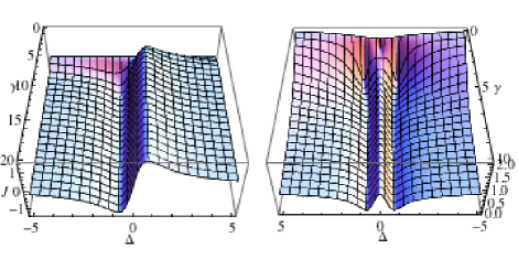
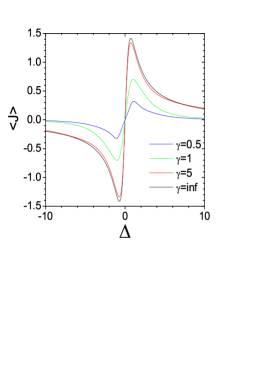
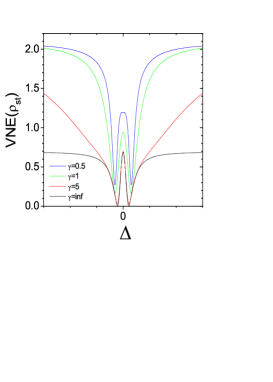
Figure 1: (Color online) Top panels. Stationary spin current $J$ (left) and von Neumann entropy (right) as a function of parameters $\gamma,\Delta$ for the open $\mathcal{H}_{XXZ}$ chain with Lindblad operators (3) and length $N=3$. Bottom panels. Sections of the spin current $J$ (left) and von Neumann entropy (right) surfaces in the top panel taken at different values of parameter $\gamma$.

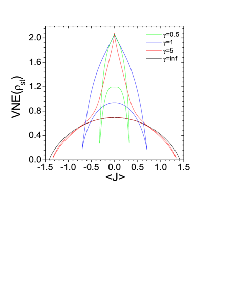
Figure 2: (Color online) Average spin current vs von Neumann entropy for different values of the coupling parameter $\gamma$. The curves are obtained as parametric plots for fixed $\gamma$ and $\Delta$ varied in the range $]-\infty,\infty[$. The VNE attains it maximum value (same for all curves) at $J=0$ and for $\Delta=\pm\infty$.

Although our approach is completely general, the rapid exponential growth of the number of algebraic equations to solve as $N$ is increased see Eq. (9), quickly restricts the application of the symmetry method to chains of small sizes. On the other hand, qubits systems with few sites can be already of potential interest for applications, and in view to the scarcity of exact results for open systems, we shall take the opportunity to investigate transport properties of these systems in exact manner for arbitrary parameters. In this respect we remark that this problem has been also investigated in previous papers using quantum trajectory method Casati2009 or direct time integrations of the Lindblad master equation PSS2012 . Our approach, being exact, is free of convergence problems of time integrations present in these alternate approaches (typically the convergence becomes very slow in the critical region $-1\leq\Delta\leq 1$ and in the weak and strong coupling limits).

In addition, the steady state density matrices for positive and negative values of the anysotropy parameter $\Delta$ are connected via relations slava

$$\rho_{s}(N,-\Delta)=U\rho_{s}^{\ast}(N,\Delta)U\text{ for }N\text{ even.}$$ (12)

$$\rho_{s}(N,-\Delta)=(\sigma^{y})^{\otimes_{N}}U\rho_{s}^{\ast}(N,\Delta)U(\sigma^{y})^{\otimes_{N}}\text{ for }N\text{ odd}$$ (13)

where $U=\sigma^{z}\otimes I\otimes\sigma^{z}\otimes....$ is a tensor product over all odd sites, which has the property $UH(\Delta)U=-H(-\Delta)$, and $\rho^{\ast}$ a complex conjugated matrix in the basis where $\sigma^{z}$ is diagonal. Note that the above transformations depend on parity of $N$ and, in particular, result in the current being an odd (even) function of $\Delta$ for odd (even) $N$,

$$j(\Delta)=(-1)^{N}j(-\Delta)$$ (14)

For the case $N=3$ the system of $d_{3}=32$ algebraic equations obtained with the help of the symmetry (8) is reported in Appendix A. From the solution of this system one can easily check that the analytical expression for the average current $J(\gamma,\Delta)=Tr(\rho(\sigma_{x}(i)\sigma_{y}(i+1)-\sigma_{y}(i)\sigma_{x}(i+1)))$ is of the form

$$J(\gamma,\Delta)=\frac{\sum_{i=0}^{N^{2}+1}\alpha_{i}(\Delta)\gamma^{2(i+1)}}{\sum_{i=0}^{N^{2}+2}\beta_{i}(\Delta)\gamma^{2i}},\;\;\;N=3,$$ (15)

with coefficients $\alpha_{i}(\Delta),\beta_{i}(\Delta)$, odd and even polynomials in $\Delta$, respectively. This implies that the current is an odd function of $\Delta$, in accordance to (14). The first leading coefficients relevant for strong and weak coupling limits are

$$\alpha_{0}(\Delta)=144\Delta^{5}(\Delta^{2}-1)^{4}(9\Delta^{2}+59),\;$$

$$\alpha_{1}(\Delta)=8\Delta^{3}(\Delta^{2}-1)^{2}(9420+13895\Delta^{2}+5822\Delta^{4}$$

$$+6561\Delta^{6}+2396\Delta^{8}+186\Delta^{10}),$$

$$\;\;\;\;\;\;\;...$$

$$\alpha_{9}(\Delta)=248832\Delta(265+96\Delta^{2}),$$

$$\alpha_{10}(\Delta)=8957952\Delta.\;$$

and

$$\beta_{0}(\Delta)=24\Delta^{4}(\Delta^{2}-1)^{4}(416+155\Delta^{2}+9\Delta^{4}),$$

$$\beta_{1}(\Delta)=2\Delta^{2}(\Delta^{2}-1)^{2}(34032+45152\Delta^{2}-7764\Delta^{4}$$

$$\;\;\;\;\;\;\;...$$

$$\beta_{10}(\Delta)=62208(228\Delta^{4}+644\Delta^{2}+355),$$

$$\beta_{11}(\Delta)=2239488(1+2\Delta^{2}).$$

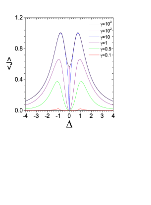
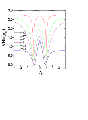
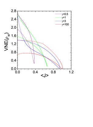
Figure 3: (Color online) Top panels.Stationary spin currents $J$ (left panel) and von Neumann entropies (right panel) vs $\Delta$ for the $\mathcal{H}_{XXZ}$ chain of length $N=4$ for different values of $\gamma$ indicated in the figure. Curves are obtained from exact stationary solution of the Lindblad Master Equation. Bottom panels. Corresponding von Neumann entropies vs stationary currents $J$ for different coupling constants $\gamma$ indicated in the panels. Bottom right panel show details of the crossover through the cusp point at which minimum of VNE and maximum of current are in exact coincidence (e.g. they occur at the same value of $\Delta$). All curves are obtained from exact stationary solutions of the Lindblad equation.

To avoid lengthy expressions we omitted other coefficients since they can be easily obtained from the exact solution of the algebraic system in Appendix A. Substituting the leading coefficients into Eq. (15) we obtain expressions for the current

$$J(\Delta,\gamma)\approx\frac{4\gamma^{2}\Delta[18(9\Delta^{2}+59)(\Delta-\Delta^{3})^{2}+\gamma^{2}F_{1}]}{12\Delta^{2}(\Delta^{2}-1)^{2}(9\Delta^{4}+155\Delta^{2}+416)+\gamma^{2}F_{2}},$$

$$J(\Delta,\gamma)\approx\frac{4\Delta(96\Delta^{2}+36\gamma^{2}+265)}{228\Delta^{4}+36\gamma^{2}(1+2\Delta^{2})+664\Delta^{2}+355},$$ (18)

valid for arbitrary values of $\Delta$ and small, $\gamma\ll 1$, and large, $\gamma\gg 1$, values of $\gamma$, respectively. Here $F_{1}=186\Delta^{10}+2396\Delta^{8}+6561\Delta^{6}+5822\Delta^{4}+13895\Delta^{2}+9420$ and $F_{2}=153\Delta^{12}+3411\Delta^{10}+19179\Delta^{8}+24007\Delta^{6}+7764\Delta^{4}+45152\Delta^{2}+34032$. Note, from the second Eq. in (18), that in the infinite coupling limit $\gamma\rightarrow\infty$ the current is:

$$\lim_{\gamma\rightarrow\infty}J(\gamma,\Delta)=\frac{4\Delta}{1+2\Delta^{2}},$$ (19)

this coinciding with the expression derived in slava by means of a perturbative approach. Similar results are obtained for other values of $N$, with the only difference that the case of $N$ even the coefficients of the series in Eq. (15) are even functions of $\Delta$, e.g. for even (odd) $N$ the current is an even (odd) function of $\Delta$. Explicit expressions of $\rho$ (and derived quantities), however, become very involved as $N$ increases since the number of algebraic equations to solve increases exponentially (see Eq. (9). Although it may be a problem to get analytical expressions for such large systems, it is not a problem to solve them numerically with very high accuracy to be considered exact for any practical purpose.

III Transport properties and von Neumann entropy for out of equilibrium finite size XXZ chains

The symmetry approach discussed above allows to obtain exact analytical results for the physical quantities of interest in the transport, such as the spin current $J$ and the von Neumann entropy $VNE(\rho_{st})=-\sum_{i}\lambda_{i}\ln\lambda_{i}$, where $\lambda_{i}$ denote the eigenvalues of the stationary reduced density matrix.

Figure 4: (Color online) Top panels. Stationary spin currents $J$ (left panel) and von Neumann entropies (right panel) vs $\Delta$ for the $\mathcal{H}_{XXZ}$ chain of length $N=5$ for different values of $\gamma$ as indicated in the figure. Curves are obtained from exact stationary solutions of the Lindblad Master Equation and, taking into account their antisymmetry property in $\Delta$, they have been plotted for positive $\Delta$ values only, just for graphical convenience). Bottom Panels. Details of the reversal current transition (left panel) and corresponding von Neumann entropy. Curves from left to right in the left panel refer to $\gamma$ values $1.9,1.95,1.96285,1.965,1.97$, respectively. Curves from top to bottom in the right panel refer to $\gamma$ values $1.8,1.9,1.97,2,2.5,3,5,6$, respectively.

In the top panels of Fig. 1 we show stationary spin current $J$ (left) and von Neumann entropy (right), as obtained from the exact solution of the system in Eq. (LABEL:systemn3) for the case $N=3$, as function functions of the parameters $\gamma,\Delta$. Sections of the spin current $J$ (left) and von Neumann entropy (right) surfaces are reported in the bottom panels for different values of parameter $\gamma$. We see that the mean current is an odd function of $\Delta$ and the VNE curve has minima very close (practically in correspondence) to maxima of $|J|$. This is clear also from Fig. 2 where a parametric curve J vs VNE is reported for different values of $\gamma$. Notice that in the strong coupling limit the VNE becomes zero exactly in correspondence to the maxima of $|J|$. This implies that optimal transport (e.g. the maximal current) is achieved in correspondence of pure states of the open $XXZ$ chain . Notice that the current vanishes for $\Delta=\pm\infty$ (Ising limit) and the VNE attains its maximum at $\Delta=0$ (free fermion point). It is also worth to note here that although analytic results are available for the Lindblad Master equation at the free fermion point Pros08 ; ZnidaricJStat2010 ; ZnidaricJPhysA ; KarevskiPatini ; ProsenZnidaric , these results do not apply to our choice of Lindblad operators (3).

Similar results, obtained for the case $N=4$, are shown in Fig. 3. We see that the spin currents $J$ (top left panel) for different values of $\gamma$ are even functions of $\Delta$, and that the von Neumann entropies (top right panel) attain their maximal value at $\Delta=\pm\infty$ where $J$ is zero, while their minima are still very close to the maxima of $|J|$. Notice from the bottom left panel, that while the minima of the VNE always reduce to zero in the strong coupling limit $\gamma\rightarrow\infty$, the correspondence between the max of $|J|$ and the min of VNE remains non exact also in this limit. This property is completely general for all $N>3$ (see below). It is also worth to note from this Fig. that as $\gamma$ is increased from small (green curve) to strong coupling limit (red curve) the VNE-$J$ curve undergoes a crossing point with the development of a cusp at a particular value of $\Delta$ for which the maximal current exactly coincides with the minimum of the VNE. This process is clearly shown in the bottom right panel of Fig. 3 where the cusp appears on the black curve $\gamma=0.85$ for $J\approx 0.6$. This folding of the curve as $\gamma$ is increased is also a general property observed for other values of $N$.

Figure 5: (Color online) The von Neumann entropy VNE vs stationary current $J$ for the open $\mathcal{H}_{XXZ}$ chain of length $N=5$ with different coupling constants $\gamma$ as indicated in the panels.The curves are obtained as parametric plots for fixed $\gamma$ and $\Delta$ varied in the range $]-\infty,\infty[$. From panel insets one can see that the minima of the VNE are always very close to maxima of the absolute value of the current. As the coupling constant $\gamma$ is increased the values of the VNE at the minima decrease and in the strong coupling limit $\gamma\rightarrow\infty$ they reduce exactly to zero (pure states).

As $N$ is increased, however, curves becomes more and more complicated with the occurrence of the interesting phenomenon of current reversal. This is first observed for the case $N=5$ reported in Figs. 4, 5 where the spin current $J$ and the von-Neumann entropy VNE, are depicted both as explicit and as implicit functions of $\Delta$. From the top left panel of Fig. 4 we see that, quite interestingly, the system undergoes current reversals in the critical region $-1\leq\Delta\leq 1$ (see the reversal occurring at $\Delta\approx 0.4$), this increasing by two the number of peaks of $|J|$ discussed for the $N=3,4$ cases (notice that, due to the antisymmetry of $J(\Delta)$ for $N$ odds, we restricted these figures to the range $\Delta\geq 0$).

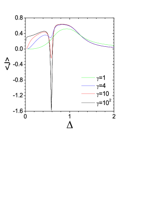
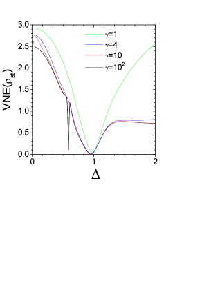
Figure 6: (Color online) Top panels.Stationary spin currents $J$ (left panel) and von Neumann entropies (right panel) vs $\Delta$ for the $\mathcal{H}_{XXZ}$ chain of length $N=6$ for different values of $\gamma$. Curves are obtained from exact stationary solution of the Lindblad Master Equation. Due to the parity of $J(\Delta)$ for $N$ even, we have restricted the figure to the range $\Delta\geq 0$ only.

The negative peaks in the current correspond to a relative minima appearing in the VNE curve, as one can see from the top right panel of this figure. Notice, however, that the correspondence between secondary peaks of $|J|$ and corresponding VNE minima occurs with delay in $\gamma$ (notice that there exist tiny minima in $J$ which have no corresponding minima in the VNE curve). Details of the current reversal phase transition and the behavior of the corresponding VNE curves are reported in the bottom panels of Fig. 4 for different values of the coupling parameters. Also, in Fig. 5 we have depicted the VNE vs stationary current $J$ as parametric plots for fixed $\gamma$ and $\Delta$ varied in the range $]-\infty,\infty[$.

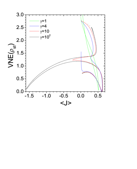
Figure 7: (Color online) von Neumann entropy VNE vs stationary current $J$ for the open $\mathcal{H}_{XXZ}$ chain of length $N=6$ for coupling constants $\gamma$ as indicated in the panels. As the coupling constant $\gamma$ is increased the values of the VNE at the two minima decrease and in the strong coupling limit $\gamma\rightarrow\infty$ they reduce exactly to zero (pure states).

From the panel insets one can see that the minima of the VNE are always very close to maxima of the absolute value of the current. As the coupling constant $\gamma$ is increased the values of the VNE at the minima decrease and in the strong coupling limit $\gamma\rightarrow\infty$ they reduce exactly to zero (pure states), in analogy with the cases $N=3,4$ discussed before.

Similar behavior, with appearance of reversal currents in the critical region is observed also for the case $N=6$, as one can see from Fig. 6. The appearance of the reversal current can be seen as a precursor of a quantum phase transition driven by the boundaries as the coupling parameter is varied. As a general rule we conjecture that the number of extrema of $|J|$ is at most $N-2$ times for $N$ even and $N-1$ times for N odd. These extrema occur always in the critical region and may disappear as the coupling constant is decreased.

IV Discussion and Conclusions

We have investigated the transport properties of an Heisenberg XXZ chain in contact with twisted XY-boundary magnetic reservoirs by means of the Lindblad master equation. Exact solutions for the stationary density matrix have been constructed for chains of small sizes using the quantum symmetry of the system. Using these solutions we have investigated the transport property of the chain in terms of the von Neumann entropy. As a result we have shown that the maximal spin current always occurs in the proximity of a minimum of the VNE and for particular choices of the anisotropy parameters it can exactly coincide with it. More precisely, we found that as the coupling constant increases, the VNE-$J$ curve undergoes a crossing point with the development of a cusp for a particular value of $\Delta$ for which the maximal current is in exact coincidence with the minimum of the VNE. We also showed the existence of current reversals e.g. the presence of negative peaks in current, which correlate to relative minima in the VNE curve, when the anisotropy parameter is in the critical region $-1\leq\Delta\leq 1$. These relative minima disappear in the small coupling limit, while in the infinite coupling limit we show that the minima of the VNE becomes exactly zero, meaning that maximal transport in this case is achieved with states very close to pure states.

Appendix A Exact stationary density matrix elements for the case $N=3$

One can check that the most general form of the density matrix compatible with the symmetry operation $T$ in Eq. (4) for the case $N=3$, is

$$\rho=\left(\begin{array}[]{cccccccc}a_{11}&a_{12}+ib_{12}&a_{13}+ib_{13}&a_{14}+ib_{14}&a_{15}+ib_{15}&a_{16}+ib_{16}&a_{17}+ib_{17}&(1-i)a_{18}\\ a_{12}-ib_{12}&a_{22}&a_{23}+ib_{23}&(1+i)a_{24}&a_{25}+ib_{25}&a_{26}+ib_{26}&a_{27}+ib_{27}&ib_{14}-a_{14}\\ a_{13}-ib_{13}&a_{23}-ib_{23}&a_{33}&ia_{26}+b_{26}&a_{35}+ib_{35}&(1+i)a_{36}&a_{37}+ib_{37}&ib_{16}-a_{16}\\ a_{14}-ib_{14}&(1-i)a_{24}&b_{26}-ia_{26}&a_{22}&b_{27}-ia_{27}&a_{23}+ib_{23}&a_{25}+ib_{25}&ia_{12}+b_{12}\\ a_{15}-ib_{15}&a_{25}-ib_{25}&a_{35}-ib_{35}&ia_{27}+b_{27}&a_{55}&ia_{37}+b_{37}&(1+i)a_{57}&ib_{17}-a_{17}\\ a_{16}-ib_{16}&a_{26}-ib_{26}&(1-i)a_{36}&a_{23}-ib_{23}&b_{37}-ia_{37}&a_{33}&a_{35}+ib_{35}&ia_{13}+b_{13}\\ a_{17}-ib_{17}&a_{27}-ib_{27}&a_{37}-ib_{37}&a_{25}-ib_{25}&(1-i)a_{57}&a_{35}-ib_{35}&a_{55}&ia_{15}+b_{15}\\ (1+i)a_{18}&-a_{14}-ib_{14}&-a_{16}-ib_{16}&b_{12}-ia_{12}&-a_{17}-ib_{17}&b_{13}-ia_{13}&b_{15}-ia_{15}&a_{11}\\ \end{array}\right)$$ (20)

This can be easily proved by substituting an arbitrary form of $\rho$, e.g. with arbitrary diagonal real elements, $a_{ii}$, and arbitrary off diagonal complex elements, $a_{ij}+ib_{ij}$, into Eq. (8) and by imposing the equality. This gives the set of relations reported in Eqs. (10), (11) and made explicit in the above $\rho$.

The exact expressions of $\rho_{ij}$ are obtained by substituting (A1) into the Lindblad master equation and by imposing the stationarity. This gives the following system of algebraic equations :

$$2(a_{14}-a_{17})+2(b_{14}+b_{17})+a_{27}-b_{27}+6a_{18}=0,$$

$$2a_{11}-a_{22}-a_{55}=0,$$

$$\gamma(2a_{22}-a_{11}-a_{33})+4b_{23}=0,$$

$$\gamma(2a_{55}-a_{11}-a_{33})-4b_{3,5}=0,$$

$$\gamma(2a_{33}-a_{22}-a_{55})+4(b_{35}-b_{23})=0,$$

$$\gamma(2a_{24}-a_{13}-b_{13})+2(b_{26}-a_{26})=0,$$

$$\gamma(2a_{57}-a_{13}-b_{13})+2(a_{37}-b_{37})=0,$$

$$\gamma(a_{12}+b_{15}-b_{16}-3b_{25}+b_{26}+b_{37})+a_{23}-a_{35}=0,$$

$$\gamma(a_{15}+a_{26}-a_{37}-3a_{16}-b_{12})-b_{14}-b_{17}+2\Delta b_{16}=0,$$

$$\gamma(3a_{15}-a_{26})+2(b_{13}-\Delta b_{15})=0,$$

$$\gamma(3b_{12}-a_{37})-2(a_{13}-\Delta a_{12})=0,$$

$$\gamma(3a_{37}-b_{12})-2(a_{57}-a_{36}+b_{27}-\Delta b_{37})=0,$$

$$\gamma(3a_{26}-a_{15})+2(a_{24}-a_{36}+b_{27}-\Delta b_{26})=0,$$

$$\gamma(3a_{25}-a_{15}-a_{26}-a_{37}-b_{12})-b_{35}+b_{23}=0,$$

$$\gamma(2a_{13}-a_{24}-a_{57})+2(b_{12}+b_{15}-2\Delta b_{13})=0,$$

$$\gamma(2b_{13}-a_{24}-a_{57})-2(a_{12}+a_{15}-2\Delta a_{13})=0,$$ (21)

$$\gamma[2(a_{24}+a_{13})-4a_{14}-a_{17}-a_{23}]-2(b_{16}-\Delta b_{14})=0,$$

$$\gamma[2(a_{24}+b_{13})-4b_{14}+b_{17}-b_{23}]+2(a_{16}-\Delta a_{14})=0,$$

$$\gamma[2(a_{57}+a_{13})-4b_{17}+b_{14}-b_{35}]+2(a_{16}-\Delta a_{17})=0,$$

$$\gamma[2(a_{57}+b_{13})+4a_{17}+a_{14}-a_{35}]+2(b_{16}-\Delta b_{17})=0,$$

$$\gamma[2(a_{57}+b_{13})-4a_{35}+a_{23}+a_{17}]+2(b_{25}-\Delta b_{35})=0,$$

$$\gamma[2(a_{57}+a_{13})-4b_{35}+b_{23}-b_{17}]+2(a_{33}-a_{55}-a_{25}+\Delta a_{35})=0,$$

$$\gamma[2(a_{24}+a_{13})-4a_{23}-a_{14}+a_{35}]-2(b_{25}-\Delta b_{23})=0,$$

$$\gamma[2(a_{24}+b_{13})-4b_{23}-b_{14}+b_{35}]+2(a_{22}-a_{33}+a_{25}-\Delta a_{23})=0,$$

$$\gamma[2(a_{11}+a_{55})-5b_{15}+b_{26}]+2(a_{13}-\Delta a_{15})=0,$$

$$\gamma[2(a_{11}+a_{22})-5a_{12}+b_{37}]-2(b_{13}-\Delta b_{12})=0,$$

$$\gamma[2(a_{33}+a_{22})-5b_{26}+b_{15}]+2(a_{24}+a_{27}-a_{36}-\Delta a_{26})=0,$$

$$\gamma[2(a_{33}+a_{55})-5b_{37}+a_{12}]+2(a_{36}-a_{27}-a_{57}+\Delta a_{37})=0,$$

$$\gamma[2(a_{14}-a_{17})+6a_{27}+a_{18}-a_{36}+2(b_{23}+b_{35})]+2(b_{26}-b_{37})=0,$$

$$\gamma[2(a_{23}+a_{35})-6b_{27}+a_{18}-a_{36}+2(b_{14}+b_{17})]+2(a_{26}-a_{37})=0,$$

$$\gamma[2(a_{23}+a_{35})-6a_{36}+a_{27}-b_{27}+2(b_{23}+b_{35})]-2(a_{26}-a_{37}-b_{26}+b_{37})=0,$$

$$\gamma(a_{12}+b_{15}-3b_{16}-b_{25}+b_{26}+b_{37})+a_{14}+a_{17}-2\Delta a_{16}=0,$$

for the real and imaginary parts, $a_{ij},b_{ij}$, respectively, of the density matrix elements. One can easily check that the solution becomes unique when the normalization condition $Tr(\rho)=1$ is imposed, this completely solving the problem. This approach, being general, can be used for other values of $N$.

In the limit $\gamma\rightarrow\infty$ the above set of equation simplifies and yields a compact solution for the density matrix, (see also slava ), in the form

$$\rho_{\gamma\rightarrow\infty}=\frac{1}{4}I+\frac{1}{4}(I-\sigma^{y})\otimes\frac{\Delta}{1+2\Delta^{2}}(\sigma^{x}-\sigma^{y})\otimes(I+\sigma^{x}).$$ (22)

From this expression we readily compute the eigenvalues for the reduced density matrix, $\lambda_{i}=(0,0,0,0,0,0,\lambda_{1},\lambda_{2})$ where

$$\lambda_{1,2}=\frac{1+4\Delta^{2}+4\Delta^{4}\pm 2\Delta\sqrt{2}\sqrt{1+4\Delta^{2}+4\Delta^{4}}}{2(1+4\Delta^{2}+4\Delta^{4})}.$$ (23)

At the point $\Delta=1/\sqrt{2}$, $\lambda_{1}=0,\lambda_{2}=1$ and the density matrix spectrum becomes that of a pure state. The point $\Delta=1/\sqrt{2}$ is exactly the point where the steady current attains its maximum value $max_{0\leq\Delta\leq\infty}J(\Delta)=\sqrt{2}$.

Analogous calculations for higher number of sites $N>3$ lead to similar results, with the difference that the steady state in the limit of large couplings becomes pure not exactly at the point $\Delta$ where the magnetization current has an extremum, but quite close to it. For $N=4$, the extremum of the current at $\gamma\rightarrow\infty$ reaches its maximum at the point $\Delta=(-1/4+\sqrt{3}/2)^{1/2}\approx 0.785$ while the density matrix spectrum becomes ”pure” at $\Delta^{\ast}=\sqrt{3}/2\approx 0.866$. Note however that the maximum peak $J(\Delta)$ is rather broad in this case, so that the maximal $j$ value and its value at the ”pure” point $J(\Delta^{\ast})$ are very close, $(J_{\max}-$ $J(\Delta^{\ast}))/J_{\max}\approx 0.009$. At $N=5$, there are two extrema, at $\Delta_{1,2}\approx 0.384,0.814$, while the state becomes pure at the points $\Delta_{1,2}^{\ast}\approx 0.383,0.924$. In the point $\Delta_{1}\approx 0.384$ the peak is narrow, and so $\Delta_{1}\approx\Delta_{1}^{\ast}$, while the second peak at $\Delta_{2}\approx 0.814$ is broad one, justifying the discrepancy between the $\Delta_{1}$ and $\Delta_{2}^{\ast}$ (data not shown).

References

• (1) H.-P. Breuer and F. Petruccione, The Theory of Open Quantum Systems, Oxford University Press, (2002).
• (2) M.B. Plenio and P.L Knight, Rev. Mod. Phys. 70, 101 (1998).
• (3) F. Heidrich-Meisner, A. Honecker, and W. Brenig, Eur. Phys. J. Special Topics 151, 135 (2007), and references therein.
• (4) X. Zotos, J. Phys. Soc. Jpn. Supp. 74, 173 (2005) and references therein.
• (5) X. Zotos and P. Prelovsek, Phys. Rev. B 53, 983 (1996).
• (6) B. N. Narozhny, A. J. Millis, and N. Andrei, Phys. Rev. B 58, R2921 (1998).
• (7) B. S. Shastry and B. Sutherland, Phys. Rev. Lett. 65, 243 (1990).
• (8) A. Klumper, Lect. Notes Phys. 645, 349 (2004).
• (9) X. Zotos, Phys. Rev. Lett. 82, 1764 (1999); J. Benz, T. Fukui, A. Klümper and C. Scheeren, J. Phys. Soc. Jpn. Suppl. 74, 181 (2005).
• (10) T. Antal, Z. Rácz and L. Sasvári, Phys. Rev. Lett. 78, 167 (1997).
• (11) T. Antal, Z. Rácz, A Rákos, and G. M. Schütz, Phys. Rev. E. 57, 5184 (1998).
• (12) P. Prelovšek, S. El Shawish, X. Zotos, and M. Long , Phys. Rev. B 70, 205129 (2004).
• (13) J.V. Alvarez and C. Gros, Phys. Rev. Lett. 88, 077203 (2002).
• (14) G. Benenti, G. Casati, T. Prosen, D. Rossini, Europhys. Lett. 85, 37001 (2009).
• (15) V. Popkov, M. Salerno, and G. Schütz, Phys. Rev E 85, 031137 (2012).
• (16) V. Popkov, A sign alternation in magnetization current in driven XXZ chains with twisted XY boundary gradients, arXiv:1210.4555v1 (2012).
• (17) T. Prosen, Phys. Scr. Lett. 86, 058511 (2012).
• (18) V. Popkov and M. Salerno, Phys. Rev. A 71, 012301 (2005); V. Popkov and M. Salerno, Europhys. Lett. 84, 30007 (2008); M. Salerno and V. Popkov, Phys. Rev. E 82, 011142 (2010).
• (19) T. Prosen, New. J. Phys. 10, 043026 (2008).
• (20) M. Žnidarič, J. Stat. Mech. L05002 (2010).
• (21) M. Žnidarič, J. Phys. A, 43 415004 (2010).
• (22) D. Karevski and T. Platini, Phys. Rev. Lett. 102, 207207 (2009).
• (23) T. Prosen and M. Žnidarič, Phys. Rev. Lett. 105, 060603 (2010).