The stability of the triangular libration points for the plane circular restricted three-body problem with light pressure

Abstract

We study the fourth-order stability of the triangular libration points in the absence of resonance for the three-body problem when the infinitesimal mass is affected not only by gravitation but also by light pressure from both primaries. A comprehensive summary of previous results is given, with some inaccuracies being corrected. The Lie triangle method is used to obtain the fourth-order Birkhoff normal form of the Hamiltonian, and the corresponding complex transformation to pre-normal form is given explicitly. We obtain an explicit expression for the determinant required by the Arnold-Moser theorem, and show that it is a rational function of the parameters, whose numerator is a fifth-order polynomial in the mass parameter. Particular cases where this polynomial reduces to a quartic are described. Our results reduce correctly to the purely gravitational case in the appropriate limits, and extend numerical work by previous authors.

1 Introduction

Stars (including the Sun) exert not only gravitation, but also radiation pressure on nearby bodies. At the same time, it is well known that dust particles are characterized by a considerable sailing capacity (cross-section to mass ratio), and hence are subject to a sizable effect of light pressure from the star, being one of the possible mechanisms for the formation and evolution of gas-dust clouds.

In the classical planar restricted circular three-body problem, two large masses, $m_{1}$ and $m_{2}$, rotate in planar circular Keplerian orbits, while a third particle of negligible mass moves in the same plane as the two larger bodies under their gravitational pull. However the classical model of the restricted three-body problem is not valid for studying the motion of material points in the solar system where the third mass has considerable sailing capacity (for example cosmic dust, stellar wind, etc). Thus it is reasonable to modify the classical model by superposing a radiative repulsion field, whose source coincides with the source of the gravitational field (the Sun), onto the gravitational field of the main body.

This problem was called the photo-gravitational restricted three-body problem by Radzievskii [19]. In a later work [20], Radzievskii performed a complete treatment of the behavior of the equilibrium points. In both papers, however, Radzievskii, who was primarily interested in the solar problem, only treated a limited range of radiation pressure parameters (in particular when only one massive body is luminous) and did not consider the question of the linear stability of the equilibrium points.

The photogravitational restricted three-body problem has been treated by several authors. In 1970 Chernikov [5] investigated the stability of the collinear equilibrium points $L_{1}$, $L_{2}$, and $L_{3}$, as well as the $L_{4}$ and $L_{5}$ points, and discussed the modifications of the results brought about through the Poynting-Robertson effect, but again only for the Sun-planet problem. Later, in 1985, Simmons et al. [23] investigated the existence and linear stability of the libration points. while, in 1996, Khasan [8] studied librational solutions of the photogravitational restricted three body problem by considering both primaries as radiating bodies.

Nonlinear stability of the triangular libration points was investigated by Kumar and Choudhry [10], who extended the work of Radzievskii by analyzing the stability of the triangular points for all values of the parameters which describe the radiating effects of the primaries. They found that, except for some cases, the motion is stable for all values of the radiation reduction factors and for all values of $\mu<0.0285954\$. They also studied [11] the stability of $L_{4}$ and $L_{5}$ under the resonance conditions $\omega_{1}=2\omega_{2}$ and $\omega_{1}=3\omega_{2}$. Later, Goździewski et al. [7] also studied the nonlinear stability of the triangular libration points. Their study of the stability of the libration points when the resonances do not exist, and in the fourth order resonance case, shows that for some values of parameters these points are stable, and for others they are unstable. In the case when the third order resonances exist, the triangular libration points are always unstable.

Kunitsyn and Polyakhova [12] gave a retrospective review of many aspects of the libration point positions and their stability for all values of radiation pressure and mass ratios.

In this paper we investigate the Lyapunov stability of the triangular solutions for all possible values of the reduction coefficients given by $\kappa_{1}$ and $\kappa_{2}$, which represent the ratios of the difference between the gravitational force and the radiative force of the bodies of mass $m_{1}$ and $m_{2}$, respectively.

We would like to stress here that some results presented in this paper have been obtained in the above references. The results of this paper should be viewed as a step towards describing the dynamics of the photogravitational restricted three-body problem. We note that, seen as a whole, the problem displays a number of interesting features that are not apparent in previous treatments.

The paper is organized as follows: section 2 contains preliminaries, where we recall the earlier results on the photogravitational planar restricted three body problem, and introduce the Hamiltonian function and the equilibria of the system, along with the condition on the masses and radiation pressure values for the stability of the linearized problem.

In Section 3, the study of the existence and linear stability of equilateral libration points is presented.

Finally, in Section 4, we apply the Arnold-Moser theorem to examine the condition of non-linear stability, excluding the resonance cases up to the fourth order. We obtain a condition for stability in the parameter space of $\kappa_{1}$, $\kappa_{2}$ and $\mu$ which may be expressed as a quintic in $\mu$, plot the relevant surface, and show that this polynomial reproduces the classical result of Deprit and Deprit-Bartholomé [6] when $\kappa_{1}=\kappa_{2}=1$. Special cases when this polynomial reduces to a quartic (and therefore explicit algebraic expressions for the surface may be obtained) are determined.

2 Hamiltonian formulation

We consider an infinitesimal mass particle moving in the photogravitational field of two masses, termed the primaries, $m_{1}$ and $m_{2}$, with both masses in circular orbits around their common center of mass. The two primaries are sources of radiation, with the parameters $\kappa_{1}$ and $\kappa_{2}$ characterizing the radiation effect of $m_{1}$ and $m_{2}$ respectively. Similar to the planar classical case, the motion of the infinitesimal mass takes place in the same plane of the primaries.

We should note that, in contrast to the classical restricted three-body problem, in the photogravitational problem the force acting on the particle depends not only on the parameters of the stars (temperature, size, density, etc.) but also on the parameters of the particle itself (size, density, etc.)

The photogravitational version of the restricted problem presented here is derived in a similar way to the classical problem (see [26]): in fact we start from a presentation and notation very similar to that used by Simmons [23]. Units are chosen so that the unit of mass is equal to the sum of the primary masses, $m_{1}+m_{2}=1$, the unit of length is equal to their separation, and the unit of time is such that the angular velocity $\omega=1$. We also set the gravitational constant $G=1$. For definiteness we also take $\mu=m_{2}/(m_{1}+m_{2})$, $0\leq\mu\leq 1$ so that $m_{1}=1-\mu$ and $m_{2}=\mu$.

We have fixed the center of mass at $(0,0)$ and the primaries, $m_{1}$ and $m_{2}$, at $(-\mu,0)$ and $(1-\mu,0)$, respectively. The forces experienced by a test particle in the coordinate system rotating with $\omega=1$ and origin at the center of mass are then derivable from the potential

$$U(x,y)=\frac{1}{2}(x^{2}+y^{2})+\frac{\alpha(1-\mu)}{r_{1}}+\frac{\beta\mu}{r_{2}},$$ (1)

where $(x,y)$ are the coordinates of the test particle,

$$r_{1}^{2}=(x+\mu)^{2}+y^{2},\qquad r_{2}^{2}=(1-x-\mu)^{2}+y^{2}$$

are the distances from the masses $m_{1}$ and $m_{2}$, respectively, and $\alpha$, $\beta$ represent the effects of the radiation pressure from the two primaries.

The Jacobi constant of the problem is given by

$$C_{J}(x,y,\dot{x},\dot{y})=\frac{1}{2}(\dot{x}^{2}+\dot{y}^{2})+\frac{1}{2}(x^{2}+y^{2})+\frac{\alpha(1-\mu)}{r_{1}}+\frac{\beta\mu}{r_{2}}.$$ (2)

After introducing the canonical coordinate system $(x,y,p_{x},p_{y})$

$$p_{x}=\frac{dx}{dt}-y,\quad p_{y}=\frac{dy}{dt}+x$$

one obtains the Hamiltonian function

$$H(x,y,p_{x},p_{y})=\frac{1}{2}(p_{x}^{2}+p_{y}^{2})+p_{x}y-p_{y}x+\frac{\alpha(1-\mu)}{r_{1}}+\frac{\beta\mu}{r_{2}}.$$ (3)

In this canonical formulation the problem of determining the libration points consists of finding all real solutions of the system of four algebraic equations given by setting the Hamiltonian equations of motion equal to zero, that is

$$p_{x}+y=0,\qquad p_{y}-x=0,$$

$$- p_{y}+\frac{\alpha(1-\mu)(x+\mu)}{r_{1}^{3}}+\frac{\beta\mu(x-1+\mu)}{r_{2}^{3}}=0,$$ (4)

$$p_{x}+\left(\frac{\alpha(1-\mu)}{r_{1}^{3}}+\frac{\beta\mu}{r_{2}^{3}}\right)y=0.$$

For later convenience we introduce the parameters $\kappa_{1}^{3}=\alpha$ and $\kappa_{2}^{3}=\beta$ as used by Schuerman [22]. Defining

$$b\equiv\displaystyle{1-\left(\frac{\kappa_{1}^{2}+\kappa_{2}^{2}-1}{2\kappa_{1}\kappa_{2}}\right)^{2}},$$ (5)

we find that the solution of (2) for the coordinates of the triangular libration points $L_{4}$ and $L_{5}$ is (see [10]):

$$x_{L_{4}}=x_{L_{5}}=\displaystyle{\frac{\kappa_{1}^{2}+1-\kappa_{2}^{2}}{2}-\mu},\qquad p_{x_{L_{4}}}=-p_{x_{L_{5}}}=-\kappa_{1}\kappa_{2}\sqrt{b},$$

$$y_{L_{4}}=-y_{L_{5}}=\kappa_{1}\kappa_{2}\sqrt{b},\quad\qquad p_{y_{L_{4}}}=p_{y_{L_{5}}}=x_{L_{4}}.$$

This implies that

$$r_{1}=\alpha^{1/3}=\kappa_{1},\quad\quad r_{2}=\beta^{1/3}=\kappa_{2},$$ (7)

showing that a necessary condition for the existence of triangular points is $\kappa_{1}\geq 0$ and $\kappa_{2}\geq 0$ (see [23]). In fact, as shown by Schuerman [22], the points lie at the intersections of the circles defined by (7), and so they exist provided further that $\kappa_{1}+\kappa_{2}\geq 1$. We remark that the existence of the equilibrium solutions is critically governed by the numerical value of $b$.

These points are the vertices of two triangles, of sides $\kappa_{1}$, $\kappa_{2}$ and $1$, based on the line joining the primaries, and so $L_{4}$ and $L_{5}$ are known as triangular (Lagrange) libration points. If we set $\alpha=1$ and $\beta_{2}=1$, the restricted photogravitational three body problem is reduced to the classical case. We consider here only the stability of $L_{4}$, however all conclusions about the stability of $L_{4}$ can be extended to $L_{5}$ just applying the symmetries of the photogravitational problem, namely

$$(x,y,p_{x},p_{y},t)\mapsto(x,-y,-p_{x},p_{y},t).$$ (8)

3 Linear stability

To investigate the stability we use Birkhoff’s procedure [3] for normalizing the Hamiltonian in a neighborhood of the libration point. We start the study of stability by finding the first order variational equations, which we then use to determine the eigenvalues. By the Arnold-Moser theorem (see [16]), it is known that a necessary condition for stability of the $L_{4}$ point is that all eigenvalues should be pure imaginary.

Using a linear canonical transformation, we first shift the origin of the coordinate system to the $L_{4}$ point and expand the Hamiltonian in a power series of the coordinates. To this end we define new coordinates $q_{1}$, $q_{2}$, $p_{1}$, $p_{2}$ by

$$x=x_{L_{4}}+q_{1},\quad \quad p_{x}=p_{x_{L_{4}}}+p_{1},$$

$$y=y_{L_{4}}+q_{2},\quad \quad p_{y}=p_{y_{L_{4}}}+p_{2},$$

in terms of which the equations of motion are

$$\frac{dq_{i}}{dt}=\frac{\partial H}{\partial p_{i}},\qquad\frac{dp_{i}}{dt}=-\frac{\partial H}{\partial q_{i}},\qquad i=1,2.$$

In these new variables the solution (2) corresponds to the equilibrium state $q_{j}=p_{j}=0$, for $j=1,2$.F We now expand the Hamiltonian in a power series of the coordinates, up to fourth order. Since the expansion is made in the neighborhood of an equilibrium point, the constant term (the value of the Hamiltonian at equilibrium) can be neglected, and the linear part must vanish. The expanded Hamiltonian can be written as

$$H=\sum_{j=0}^{\infty}H_{j},$$ (9)

where $H_{j}$ are homogeneous polynomials of degree $j$ in the new variables. Calculating this expansion to fourth order we find

$$H_{0} =H(x_{L_{4}},y_{L_{4}},p_{x_{L_{4}}},p_{y_{L_{4}}}),$$

$$H_{1} =0,$$

$$H_{2} =\tfrac{1}{2}(p_{1}^{2}+p_{2}^{2})+q_{2}p_{1}-q_{1}p_{2}+\left(A-\tfrac{1}{4}\right)q_{1}^{2}+Bq_{1}q_{2}-\left(A+\tfrac{1}{4}\right)q_{2}^{2},$$

$$H_{3} =h_{3000}\;q_{1}^{3}+h_{2100}\;q_{1}^{2}q_{2}+h_{1200}\;q_{2}^{2}q_{1}+h_{0300}\;q_{2}^{3},$$

$$H_{4} =h_{4000}\;q_{1}^{4}+h_{3100}\;q_{1}^{3}q_{2}+h_{2200}\;q_{2}^{2}q_{1}^{2}+h_{1300}\;q_{1}q_{2}^{3}+h_{0400}\;q_{2}^{4},$$

where

$$A \equiv -\frac{3}{4}+\frac{3b}{2}\left[\mu\kappa_{1}^{2}+(1-\mu)\kappa_{2}^{2}\right],$$

$$B \equiv -\frac{3}{2}\,\frac{\sqrt{b}}{\kappa_{1}\kappa_{2}}\left[(1-\mu)\kappa_{2}^{2}(\kappa_{1}^{2}+1-\kappa_{2}^{2})+\mu\kappa_{1}^{2}(\kappa_{2}^{2}+1-\kappa_{1}^{2})\right].$$ (10)

The values of $A$ and $B$ used in $H_{2}$ are conveniently defined for simplifying expressions which appear later. The coefficients of $H_{3}$ and $H_{4}$, calculated using Maple, coincide with those given in Kumar and Choudhry [10] and are listed in Appendix A.

The system of linear differential equations derived from the quadratic term, $H_{2}$, describes the tangent flow around $L_{4}$. Linear stability is determined by the character of the associated eigenvalues, which are the roots of the characteristic equation

$$\lambda^{4}+\lambda^{2}+9\mu(1-\mu)\,b=0,$$ (11)

whose eigenvalues are found to be

$$\lambda_{1,2} =\pm\sqrt{-\frac{1}{2}+\frac{\sqrt{1-36\mu(1-\mu)b}}{2}}\;,$$

$$\lambda_{3,4} =\pm\sqrt{-\frac{1}{2}-\frac{\sqrt{1-36\mu(1-\mu)b}}{2}}\;.$$

For linear stability all of these eigenvalues should be pure imaginary, which is the case if

$$0\leq 36\mu(1-\mu)b\leq 1.$$ (13)

Substituting (5) in (13), we obtain

$$1-\left(\frac{\kappa_{1}^{2}+\kappa_{2}^{2}-1}{2\kappa_{1}\kappa_{2}}\right)^{2}\leq\frac{1}{36\mu(1-\mu)}\Rightarrow\left(\frac{\kappa_{1}^{2}+\kappa_{2}^{2}-1}{2\kappa_{1}\kappa_{2}}\right)^{2}\geq\frac{-36\mu^{2}+36\mu-1}{36\mu(1-\mu)}.$$ (14)

Since the left-hand side can be zero, we require

$$\frac{-36\mu^{2}+36\mu-1}{36\mu(1-\mu)}\leq 0\Rightarrow 36\mu^{2}-36\mu+1\geq 0,$$ (15)

as $\mu\in[0,1]$. This equation is satisfied for $\mu\leq\frac{1}{2}-\frac{\sqrt{2}}{3}$ and $\mu\geq\frac{1}{2}+\frac{\sqrt{2}}{3}$, and so, in these subintervals, the eigenvalues (3) are distinct and pure imaginary.

Throughout this paper, we restrict ourselves to the case

$$\mu\leq\frac{1}{2}-\frac{\sqrt{2}}{3}\approx 0.0285954\equiv\mu^{*}$$

for which the linear stability conditions are fulfilled for all values of $\kappa_{1}$ and $\kappa_{2}$.

Note that Lagrange’s classical criterion for stability is recovered in the limit of no radiation pressure ($\kappa_{1}\rightarrow 1$, $\kappa_{2}\rightarrow 1$, $b\rightarrow 3/4$). In this case the inequality (14) for the existence of two pairs of pure imaginary values becomes

$$27\mu(1-\mu)\leq 1,\quad\mbox{or equivalently}\quad\mu(1-\mu)\leq 1/27.$$

We remark that this result implies the stability of the $L_{4}$ point in the classical planar circular restricted three-body problem when the mass ratio parameter satisfies $0<\mu<\mu_{R}=\frac{1}{2}(1-\frac{\sqrt{69}}{9})\approx 0.0385208$, where $\mu_{R}$ is known as the Routh value.

We write the four eigenvalues as $\pm i\omega_{1}$, $\pm i\omega_{2}$ where the strictly positive numbers $\omega_{1}$ and $\omega_{2}$ (frequencies) are determined by the set of relations

$$\omega_{1}^{2}=-\lambda_{1,2}^{2}=\frac{1+M}{2},\qquad\omega_{2}^{2}=-\lambda_{3,4}^{2}=\frac{1-M}{2},$$ (16)

where $M\equiv\sqrt{1-36\mu(1-\mu)b}$. The expressions (16) show that

$$0<\omega_{2}<\frac{1}{\sqrt{2}}<\omega_{1}<1.$$ (17)

We remark that $\omega_{1}$ and $\omega_{2}$ and the coefficients of all $H_{j}$ are functions of the parameters $\mu$, $\kappa_{1}$ and $\kappa_{2}$.

4 Normal form and non-linear stability

Having established linear stability, the next step is to transform the Hamiltonian into its Birkhoff normal form. This normalization allows us to apply Arnold’s theorem [1] to investigate the stability of the $L_{4}$ point for mass ratios $\mu<\mu^{*}$, except for the resonant cases. From the coefficients of the normal form, Arnold’s thorem constructs a determinant, $D$, defined later, which, when non-zero, establishes the stability of the equilibrium point. To obtain the Birkhoff normal form we use the Lie series method, with the calculations being performed using Maple. To determine the domain of applicability of the results, it is necessary to obtain the resonances, which we now calculate.

4.1 Existence of resonances

In this section we study the values for which the frequencies at the equilibrium are in resonance. Since we are working to fourth order in the normal form, we thus need to consider resonances up to fourth order of the triangular libration points.

The stability analysis of the $L_{4}$ point can be carried out if the frequencies $\omega_{1}$, $\omega_{2}$ satisfy the non-resonance condition

$$c_{1}\omega_{1}+c_{2}\omega_{2}\neq 0$$ (18)

for all integers $c_{1}$, $c_{2}$ such that $|c_{1}|+|c_{2}|\leq 4$. This condition is violated for $\omega_{1}=2\omega_{2}$ and $\omega_{1}=3\omega_{2}$, and, obviously when $\omega_{1}=\omega_{2}$.

We start the discussion by noting that the first-order resonance appears when one of the frequencies is zero. In our case, this is possible if either $\mu=0$ or $\kappa_{1}+\kappa_{2}=1$. For $\mu=0$ the restricted photogravitational three body problem is reduced to Kepler’s problem in a rotating coordinate frame. The $L_{4}$ point in this case is evidently unstable in the sense of Lyapunov.

The second case has no classical equivalent: $L_{4}$ and $L_{5}$ coincide with the inner collinear point $L_{1}$ (see Simmons et. al. [23]). In particular if $\kappa_{2}=1$ and $\kappa_{1}\rightarrow 0$ the libration points $L_{4}$ and $L_{5}$ move from their classical equilateral positions onto the luminous mass and coalesce there with the inner libration point $L_{1}$. It is clear that the motion will be unstable.

We have seen above that if $\kappa_{1}=\kappa_{2}=1$, then $\mu=\mu_{R}$ and the triangular libration points are stable in the sense of Lyapunov. This agrees with the result of Meyer Placián and Yaguas [17], who demonstrated the stability of the Lagrange equilateral triangle points, $L_{4}$ and $L_{5}$, in the plane circular restricted three-body problem when the mass ratio parameter is equal to $\mu=\mu_{R}$, the critical value of Routh.

We turn to the two remaining cases. The second order resonance $\omega_{1}=\omega_{2}$ occurs when $\mu=\tfrac{1}{2}\pm\sqrt{\tfrac{1}{4}-\tfrac{1}{36b}}$. Since $\mu>0$, the resonance appears for parameters $\kappa_{1}$ and $\kappa_{2}$ satisfying the condition $b\geq 1/9$. In the first graph of Figure 1 we have plotted the relevant part (i.e. with the negative root) of $\mu(b)$, together with the line $\mu=\mu^{*}$. We see that (other than at the exceptional value $b=1$) the resonant values only exist for $\mu>\mu^{*}$.

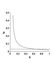
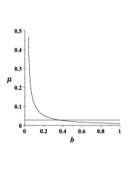
Figure 1: Graphs of $\mu(b)$ for (from left to right) the 1:1, 1:2 and 1:3 resonances. The horizontal line is $\mu=\mu^{*}$.

We use the same criterion adopted in the previous case for determining the masses for which the resonance $\omega_{1}=2\omega_{2}$ occurs. In this way, one obtains $\mu={\frac{1}{2}-\sqrt{\frac{1}{4}-\frac{4}{225b}}}$, so that the resonance appears for parameters $\kappa_{1}$ and $\kappa_{2}$ satisfying the condition $b\geq 16/225\approx 0.071$. The function $\mu(b)$ for this resonance is shown in the second graph of Figure 1. We see that $\mu(b)=\mu^{*}$ when $b=16/25=0.64$. Therefore, in contrast to the results of Kumar and Choudhry [10], who claimed that the resonance $\omega_{1}=2\omega_{2}$ occurs for values from $b=0.65$ to $b=0.95$, we find that it occurs for $b\in[0.64,1]$.

Finally, the resonance $\omega_{1}=3\omega_{2}$ occurs for $\mu={\frac{1}{2}-\sqrt{\frac{1}{4}-\frac{1}{100b}}}$. Since $\mu>0$, the resonance appears for values of $\kappa_{1}$ and $\kappa_{2}$ satisfying ${b\geq 1/50}$. In this case $\mu(b)=\mu^{*}$ for $b=9/25=0.36$. Kumar and Choudhry [10] stated that this resonance occurs for values from $b=0.4$ to $b=0.95$, but we find that, in fact, it appears for $b\in[0.36,1]$.

In Table 1 we show the values of $\mu$ for $\kappa_{1}=1$ and several values of $\kappa_{2}$ for the resonances $\omega_{1}=\omega_{2}$, $\omega_{1}=2\omega_{2}$ and $\omega_{1}=3\omega_{2}$. Note that when one of the radiation coefficients is $1$, and there is a 1:1 resonance, the points $L_{4}$ and $L_{5}$ are linearly stable with the condition that mass parameter $\mu$ is at most $0.0385209$. Our result refines that of Kumar and Choudhry [10] and has an influence on the analysis of the non-linear stability of $L_{4}$, and consequently on that of $L_{5}$.

$\kappa_{2}$	$\omega_{1}=\omega_{2}$	$\omega_{1}=2\omega_{2}$	$\omega_{1}=3\omega_{2}$
1	0.0385209	0.0349233	0.0321444
0.9	0.0361369	0.0327702	0.0301682
0.8	0.0342412	0.0310571	0.0285955
0.7	0.0327266	0.029688	0.0273381
0.6	0.0315184	0.0285955	0.0263345
0.5	0.0305638	0.027732	0.0255412
0.4	0.0298247	0.0270634	0.0249269
0.3	0.0292741	0.0265653	0.0244692
0.2	0.0288932	0.0262206	0.0241524
0.1	0.0286693	0.0260181	0.0239662

Table 1: Values of $\mu$ for $\kappa_{1}=1$.

4.2 Birkhoff’s Normal Form

In section 3 we determined the conditions under which the eigenvalues are purely imaginary, thus guaranteeing that the phogravitational Hamiltonian (3) satisfies the first condition of the Arnold-Moser theorem. The next step is the normalization procedure that transforms Hamiltonian (9) to Birkhoff’s normal form up to fourth order, excluding regions close to the resonances established in the previous section.

To this end, first we make a further change of variables,

$$(q_{1},q_{2},p_{1},p_{2})\rightarrow(\bar{\xi}_{1},\bar{\xi}_{2},\bar{\eta}_{1},\bar{\eta}_{2}),$$

to the Hamiltonian (3) that diagonalizes $H_{2}$:

$$\bar{H}=\frac{\omega_{1}}{2}(\bar{\xi}_{1}^{2}+\bar{\eta}_{1}^{2})-\frac{\omega_{2}}{2}(\bar{\xi}_{2}^{2}+\bar{\eta}_{2}^{2})+\sum_{j=3}^{m}H_{j}(\bar{\xi}_{1},\bar{\xi}_{2},\bar{\eta}_{1},\bar{\eta}_{2})+O_{m+1}.$$ (19)

We use a negative sign on the second term to emphasize the non-positive character of the photogravitational Hamiltonian.

We note that $\bar{H}_{2}$ is already in real normal form since it depends only on the actions $\bar{R}_{\nu}\equiv\bar{\xi}_{\nu}^{2}+\bar{\eta}_{\nu}^{2}$, $\nu=1,2$. Also, recall that $\omega_{1}$ and $\omega_{2}$ are the linear frequencies analyzed in the previous sections. The terms of order greater than two depend on $(\bar{\xi}_{1},\bar{\xi}_{2},\bar{\eta}_{1},\bar{\eta}_{2})$, but not necessarily in such a simple way as $\bar{H}_{2}$. The purpose of the Birkhoff normal form is to find a near identity symplectic coordinate change

$${\bf z^{(m)}}=\bar{\bf z}+\sum_{i+j+k+l=2}^{i+j+k+l=m}a_{ijkl}{\bar{\xi}_{1}}^{i}{\bar{\xi}_{2}}^{j}{\bar{\eta}_{1}}^{k}{\bar{\eta}_{2}}^{l}+O_{m+1}$$ (20)

so that the even order terms in the Hamiltonian depend on the new variables ${\bf z}=(\xi_{1},\xi_{2},\eta_{1},\eta_{2})$ in such a way that they can be grouped as powers of $R_{1}$ and $R_{2}$.

It is implicit in this last statement that the Hamiltonian system’s natural resonances have been taken into account. Let $\mathcal{S}$ be some system of resonance relations, i.e. relations of the form $\lambda_{s}=\sum_{i=1}^{n}m_{i}\lambda_{i}$ with $m_{i}$ non-negative integers not all zero. From the viewpoint of the general theory of dynamical systems, equilibria and periodic trajectories in Hamiltonian systems are all resonant. Indeed, for equilibria, if $\lambda_{1}$ is an eigenvalue of an equilibrium of a Hamiltonian system, then $\lambda_{2}=-\lambda_{1}$ is also an eigenvalue. So an infinite number of resonance relations of the form

$$\lambda_{s}=\lambda_{s}+k(\lambda_{1}+\lambda_{2}),k\in\mathbb{Z}$$

are satisfied. This means that we can find a non-divergent generating function (and consequent canonical transformation) that transforms away all terms of odd degree of the Hamiltonian (9). We have, necessarily, to retain part of the even terms corresponding to the resonant monomials that appear in (9). This will become clearer in the brief presentation of the algorithm we have used to implement the Birkhoff normal form. Of course, a truncated Birkhoff normal form is a polynomial Hamiltonian that is formally integrable, since it is expressed only in terms of the actions $R_{j}$, $j=1,\ldots,n$. For more theoretical details we refer the reader to [2] and [24], and for practical implementations, the works of [14] and [25]. In this paragraph we have tried to stress a point that is usually not made clearly when calculating the Birkhoff normal forms for the photogravitational problem: the difference between the natural resonances of the $2n$ complex eigenvalues, and the resonances of the real eigenfrequencies $\omega_{1}$ and $\omega_{2}$.

Perhaps due to Hamilton-Jacobi tradition, some engineers and physicists, for example Kumar and Choudhry [10], prefer to work with real variables and mixed generating functions which depend on both old and new variables. In this work we use the Lie derivative approach, which allows us to use a generating function dependent only on new the variables, with the advantage of turning the cumbersome passage to the normal formal more transparent. Moreover, with this approach, when the coefficients are not algebraic, but numerical, one can write fast codes to construct very high order normal forms (see for example [24], [25]).

Before describing the algorithm and the form of the generating function, a further step is necessary to prepare the Hamiltonian for the process of normalization. It is easier to perform the manipulations in the complex field and, to this end, we shall make use of the change of variables, ${\bf R_{C}}$, and its inverse, ${\bf C_{R}}$:

$${\bf R_{C}:} \quad x_{j}=\frac{1}{\sqrt{2}}(\bar{\xi}_{j}-{\bf i}\bar{\eta}_{j}), \quad y_{j}=\tfrac{1}{\sqrt{2}}(-{\bf i}\bar{\xi}_{j}+\bar{\eta}_{j}),$$

$${\bf C_{R}:} \quad\bar{\xi}_{j}=\frac{1}{\sqrt{2}}(x_{j}+{\bf i}y_{j}), \quad\bar{\eta}_{j}=\tfrac{1}{\sqrt{2}}({\bf i}x_{j}+y_{j}),$$

where ${\bf i}=\sqrt{-1}$, to transform $\bar{H}(\bar{\xi}_{1},\bar{\xi}_{2},\bar{\eta}_{1},\bar{\eta}_{2})$ into the complex Hamiltonian

$$H(x_{1},x_{2},y_{1},y_{2})={\bf i}\>\omega_{1}x_{1}y_{1}+{\bf i}\>\omega_{2}x_{2}y_{2}+\!\!\!\!\!\!\!\!\sum_{k_{1}+k_{2}+l_{1}+l_{2}=3}\!\!\!\!\!\!\!\!h_{k_{1}k_{2}l_{1}l_{2}}\;x_{1}^{k_{1}}x_{2}^{k_{2}}y_{1}^{l_{1}}y_{2}^{l_{2}}.$$ (21)

In fact, the complexification can be done directly from Hamiltonian (3) to (21), as is the case in this work (Appendix B).

Now, we introduce the generating function $G(x_{1},x_{2},y_{1},y_{2})$ as a series expansion in homogeneous polynomials of degree $m\geq 3$

$$G_{m}(x_{1},x_{2},y_{1},y_{2})=\sum_{j=3}^{m}G_{j},\quad\mbox{where}\quad G_{j}=\!\!\!\!\!\!\!\!\sum_{k_{1}+k_{2}+l_{1}+l_{2}=j}\!\!\!\!\!\!\!\!g_{k_{1}k_{2}l_{1}l_{2}}\;x_{1}^{k_{1}}x_{2}^{k_{2}}y_{1}^{l_{1}}y_{2}^{l_{2}},$$ (22)

and the associated canonical transformation $T_{G}$, such that

$$T_{G}\;H(x_{1},x_{2},y_{1},y_{2})=Z(X_{1},X_{2},Y_{1},Y_{2})=H(T_{G}(x_{1},x_{2},y_{1},y_{2})),$$

with

$$Z(X_{1},X_{2},Y_{1},Y_{2})=H+\{H,G\}+\frac{1}{2!}\{\{H,G\},G\}+\frac{1}{3!}\{\{\{H,G\},G\},G\}+\cdots,$$ (23)

where $\{H,G\}=L_{H}G$ is the usual Poisson bracket (or Lie derivative) of the functions $H$ and $G$. This means that $Z$ is the time one flow of the flux generated by the canonical system of equations associated with the generating function $G$. To find the Birkhoff normal form and the corresponding change of variables (and its inverse) one has to determine the generating function that gives the prescribed form discussed above. Collecting powers of (23) up to order four gives

$$Z_{2}= H_{2},$$

$$Z_{3}= H_{3}+\{H_{2},G_{3}\},$$ (24)

$$Z_{4}= H_{4}+\{H_{3},G_{3}\}+\frac{1}{2!}\{\{H_{2},G_{3}\},G_{3}\}+\{H_{2},G_{4}\}.$$

Since we are supposing that there are no resonances besides the natural ones (as explained above), all terms of order 3 can be removed from (23) by setting

$$\{H_{2},G_{3}\}=Z_{3}-H_{3}.$$

Solving for $Z_{3}=0$ gives

$$G_{3}=\sum_{k_{1}+k_{2}+l_{1}+l_{2}=3}\displaystyle\frac{h_{k_{1}k_{2}l_{1}l_{2}}}{({\bf k}-{\bf l},\Lambda)}\;x_{1}^{k_{1}}x_{2}^{k_{2}}y_{1}^{l_{1}}y_{2}^{l_{2}},$$ (25)

where

$$({\bf k}-{\bf l},\Lambda)={\bf i}(k_{1}-l_{1})\omega_{1}+{\bf i}(k_{2}-l_{2})\omega_{2}$$

are the coefficients of the monomials of the Poisson bracket $\{H_{2},G_{3}\}$, which are nonzero outside the resonance regions.

For terms of order four, the solution is not so easy since $Z_{4}\neq 0$, and we have to solve simultaneously for $G_{4}$ and $Z_{4}$, and so on, up to the required order, $m$, of the normal form. In this case one can use the general result [24] for $k\geq 3$:

$$\{H_{2},G_{k}\}+Z_{k}=F_{k},\qquad F_{3}=H_{3},\;Z_{2}=H_{2}$$ (26)

and

$$F_{k}=\sum_{m=1,\ldots,k-3}\frac{m}{k-2}\{G_{2+m},Z_{k-m}\}+\sum_{m=1,\ldots,k-2}\frac{m}{k-2}H_{2+m,k-m-2}$$ (27)

where

$$H_{2+m,k-m-2}=\sum_{j=1}^{k-m-2}\frac{j}{k-m-2}\{G_{2+j},H_{2+m,k-j-m-2}\}+H_{k}.$$ (28)

Applying these formulae we can find $Z_{4}$ and $G_{4}$, which give us the fourth order terms that the Arnold-Moser Theorem requires. The algebraic manipulations described so far were performed using the software Maple, but any algebraic software could have been used. Note that $Z_{4}$ is a complex Birkhoff normal form but, using the transformation $C_{R}$ given in (4.2), we obtain finally

$$Hr_{2}=\frac{\omega_{1}}{2}(\xi_{1}^{2}+\eta_{1}^{2})-\frac{\omega_{2}}{2}(\xi_{2}^{2}+\eta_{2}^{2}),$$

$$Hr_{3}=0,$$ (29)

$$Hr_{4}=\delta_{11}(\xi_{1}^{2}+\eta_{1}^{2})^{2}+\delta_{12}(\xi_{1}^{2}+\eta_{1}^{2})(\xi_{2}^{2}+\eta_{2}^{2})+\delta_{22}(\xi_{2}^{2}+\eta_{2}^{2})^{2},$$

which is the form required by the Arnold-Moser Theorem.

According to this theorem we have to check whether the determinant

$$D(\kappa_{1},\kappa_{2})=-(\delta_{11}\,\omega_{2}^{2}-2\delta_{12}\,\omega_{1}\omega_{2}+\delta_{22}\,\omega_{1}^{2})$$ (30)

is nonzero. If $D(\kappa_{1},\kappa_{2})\neq 0$ for some pair $(\kappa_{1},\kappa_{2})$ then, for this pair, the motion is stable in the Lyapunov sense provided $\omega_{1}\neq\omega_{2}$, $\omega_{1}\neq 2\omega_{2}$ or $\omega_{1}\neq 3\omega_{2}$.

The complex canonical transformation that takes the Taylor series (3) to (21) is shown in Appendix B while the coefficients of the fourth order normal form are given in Appendix C. After a sequence of algebraic manipulations we finally obtain the determinant as a rational function, whose numerator is a quintic in $\mu$. Explicitly, defining the product of factors

$$\Pi\equiv\left(\kappa_{1}+1+\kappa_{2}\right)\left(\kappa_{1}+1-\kappa_{2}\right)\left(\kappa_{1}-1+\kappa_{2}\right)\left(\kappa_{1}-1-\kappa_{2}\right),$$

we can write $D$ as

$$D(\kappa_{1},\kappa_{2})=\frac{1}{X}\sum_{i=0}^{5}D_{i}\,\mu^{i}$$

where the denominator, $X$, is

$$X=2048\,\Pi{\kappa_{1}}^{4}{\kappa_{{2}}}^{4}(225\,\Pi{\mu}(\mu-1)-16\,{\kappa_{1}}^{2}{\kappa_{2}}^{2})\left(9\,\Pi\mu(\mu-1)-{\kappa_{1}}^{2}{\kappa_{2}}^{2}\right)$$

and the coefficients, $D_{i}$, of the quintic in the numerator are given by

$$\frac{D_{5}}{12960\Pi^{3}} = (\kappa_{1}^{2}-\kappa_{2}^{2})(5\,{\kappa_{1}}^{2}-5-8\,\kappa_{1}\kappa_{2}+5\,{\kappa_{2}}^{2})(5\,{\kappa_{1}}^{2}-5+8\,\kappa_{1}\kappa_{2}+5\,{\kappa_{2}}^{2}),$$

$$-\frac{D_{4}}{2592\Pi^{2}} = 375\,{\kappa_{1}}^{2}-1500\,{\kappa_{1}}^{4}+2250\,{\kappa_{1}}^{6}-1500\,{\kappa_{1}}^{8}+375\,{\kappa_{1}}^{10}$$

$$-250\,{\kappa_{2}}^{2}+1000\,{\kappa_{2}}^{4}-1500\,{\kappa_{2}}^{6}+1000\,{\kappa_{2}}^{8}-250\,{\kappa_{2}}^{10}$$

$$-350\,{\kappa_{1}}^{2}{\kappa_{2}}^{2}+500\,{\kappa_{1}}^{2}{\kappa_{2}}^{4}-1450\,{\kappa_{1}}^{2}{\kappa_{2}}^{6}+925\,{\kappa_{1}}^{2}{\kappa_{2}}^{8}$$

$$+{\kappa_{1}}^{4}(150\,{\kappa_{2}}^{2}+8\,{\kappa_{2}}^{4}-1650\,{\kappa_{2}}^{6})+1750\,{\kappa_{1}}^{6}{\kappa_{2}}^{2}+1900\,{\kappa_{1}}^{6}{\kappa_{2}}^{4}$$

$$-1300\,{\kappa_{1}}^{8}{\kappa_{2}}^{2},$$

$$\frac{D_{3}}{288\Pi^{2}} = 3375\,{\kappa_{1}}^{2}-13500\,{\kappa_{1}}^{4}+20250\,{\kappa_{1}}^{6}-13500\,{\kappa_{1}}^{8}+3375\,{\kappa_{1}}^{10}$$

$$-1125\,{\kappa_{2}}^{2}+4500\,{\kappa_{2}}^{4}-6750\,{\kappa_{2}}^{6}+4500\,{\kappa_{2}}^{8}-1125\,{\kappa_{2}}^{10}$$

$$-6300\,{\kappa_{1}}^{2}{\kappa_{2}}^{2}+7495\,{\kappa_{1}}^{2}{\kappa_{2}}^{4}-9590\,{\kappa_{1}}^{2}{\kappa_{2}}^{6}+5020\,{\kappa_{1}}^{2}{\kappa_{2}}^{8}$$

$$+4205\,{\kappa_{1}}^{4}{\kappa_{2}}^{2}+144\,{\kappa_{1}}^{4}{\kappa_{2}}^{4}-10065\,{\kappa_{1}}^{4}{\kappa_{2}}^{6}$$

$$+14990\,{\kappa_{1}}^{6}{\kappa_{2}}^{2}+14565\,{\kappa_{1}}^{6}{\kappa_{2}}^{4}-11770\,{\kappa_{1}}^{8}{\kappa_{2}}^{2}$$

$$\frac{-D_{2}}{288\,{\kappa_{1}}^{2}\Pi} = 1125-6750{\kappa_{1}}^{2}+16875{\kappa_{1}}^{4}-22500{\kappa_{1}}^{6}+16875{\kappa_{1}}^{8}-6750{\kappa_{1}}^{10}$$

$$+1125\,{\kappa_{1}}^{12}-5400\,{\kappa_{2}}^{2}+11050\,{\kappa_{2}}^{4}-12700\,{\kappa_{2}}^{6}+8925\,{\kappa_{2}}^{8}$$

$$-3700{\kappa_{2}}^{10}+700{\kappa_{2}}^{12}+14890{\kappa_{1}}^{2}{\kappa_{2}}^{2}-9518{\kappa_{1}}^{2}{\kappa_{2}}^{4}-1634{\kappa_{1}}^{2}{\kappa_{2}}^{6}$$

$$+6012\,{\kappa_{1}}^{2}{\kappa_{2}}^{8}-3000\,{\kappa_{1}}^{2}{\kappa_{2}}^{10}-5560\,{\kappa_{1}}^{4}{\kappa_{2}}^{2}-674\,{\kappa_{1}}^{4}{\kappa_{2}}^{4}$$

$$-3712\,{\kappa_{1}}^{4}{\kappa_{2}}^{6}+7295\,{\kappa_{1}}^{4}{\kappa_{2}}^{8}-18660\,{\kappa_{1}}^{6}{\kappa_{2}}^{2}-14298\,{\kappa_{1}}^{6}{\kappa_{2}}^{4}$$

$$-12850\,{\kappa_{1}}^{6}{\kappa_{2}}^{6}+13440\,{\kappa_{1}}^{8}{\kappa_{2}}^{4}+21440\,{\kappa_{1}}^{8}{\kappa_{2}}^{2}-6710\,{\kappa_{1}}^{10}{\kappa_{2}}^{2}$$

$$\frac{-D_{1}}{32\,{\kappa_{1}}^{4}{\kappa_{2}}^{2}\Pi} = 3465-13860\,{\kappa_{1}}^{2}+20790\,{\kappa_{1}}^{4}-13860\,{\kappa_{1}}^{6}+3465\,{\kappa_{1}}^{8}$$

$$-2790\,{\kappa_{2}}^{2}-4780\,{\kappa_{2}}^{4}+4070\,{\kappa_{2}}^{6}+35\,{\kappa_{2}}^{8}$$

$$-2870\,{\kappa_{1}}^{6}{\kappa_{2}}^{2}-5196\,{\kappa_{1}}^{4}{\kappa_{2}}^{4}+2950\,{\kappa_{1}}^{4}{\kappa_{2}}^{2}$$

$$+2710\,{\kappa_{1}}^{2}{\kappa_{2}}^{2}+4566\,{\kappa_{1}}^{2}{\kappa_{2}}^{6}+15912\,{\kappa_{1}}^{2}{\kappa_{2}}^{4}$$

$$\frac{-D_{0}}{512\,{\kappa_{1}}^{6}{\kappa_{2}}^{4}} = 5-20\,{\kappa_{1}}^{2}+30\,{\kappa_{1}}^{4}-20\,{\kappa_{1}}^{6}+5\,{\kappa_{1}}^{8}+10\,{\kappa_{2}}^{2}-36\,{\kappa_{2}}^{4}+22\,{\kappa_{2}}^{6}$$

$$-{\kappa_{2}}^{8}-10\,{\kappa_{1}}^{2}{\kappa_{2}}^{2}+56\,{\kappa_{1}}^{2}{\kappa_{2}}^{4}+22\,{\kappa_{1}}^{2}{\kappa_{2}}^{6}-10\,{\kappa_{1}}^{4}{\kappa_{2}}^{2}$$

$$-36\,{\kappa_{1}}^{4}{\kappa_{2}}^{4}+10\,{\kappa_{1}}^{6}{\kappa_{2}}^{2}$$

Since the numerator of $D$ is a polynomial of order 5, it is, in general, impossible to write an algebraic expression for the values for which $\mu(\kappa_{1},\kappa_{2})$ produces $D=0$. However it is easy to plot the surface $D=0$, which is shown in figure 2 for the parameter ranges $\kappa_{1}\in[0,1]$, $\kappa_{2}\in[0,1]$, $\mu\in[0,0.3]$.

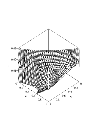
Figure 2: The surface $D(\mu,\kappa_{1},\kappa_{2})=0$.

This surface seems to be equivalent to that shown by Goździewski et. al. [7], who use slightly different variables. They, however, do not give an explicit expression for the determinant (their $D_{4}$), while our expression allows a better understanding of the structure of this function. For example it is possible to see that, for certain combinations of $\kappa_{1}$ and $\kappa_{2}$, the numerator of $D$ reduces to a quartic, and an explicit algebraic expression for $\mu(\kappa_{1},\kappa_{2})$ on the surface $D=0$ can be obtained. In the physical region of the parameter space this happens when

$$\kappa_{1}+\kappa_{2}=1,\qquad\kappa_{1}=\kappa_{2},~{}~{}~{}{\rm or}~{}~{}~{}~{}5(\kappa_{1}^{2}+\kappa_{2}^{2}-1)+8\kappa_{1}\kappa_{2}=0.$$

The second of these is particularly interesting, since it includes the purely gravitational case $\kappa_{1}=\kappa_{2}=1$. For these values we have

$$D=D_{c}={\frac{9}{64}}\,{\frac{13041\,{\mu}^{4}-26082\,{\mu}^{3}+14664\,{\mu}^{2}-1623\,\mu+16}{\left(675\,{\mu}^{2}-675\,\mu+16\right)\left(27\,{\mu}^{2}-27\,\mu+1\right)}},$$

with the first positive root at

$$\mu=\frac{1}{2}-{\frac{1}{2898}}\,\sqrt{1576995+966\,\sqrt{199945}}\approx 0.0109136676$$

in agreement with the classical result of Deprit and Deprit-Bartholomé. For illustration we show the behavior of $D_{c}(\mu)$ in Figure 3.

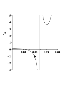
Figure 3: The classical determinant, $D_{c}$, for $0\leq\mu\leq 0.04$

5 Conclusion

One of the motivations of this paper was to bring together various results relating to the restricted photogravitational three-body problem scattered about the literature, with special emphasis on the stability of the $L_{4}$ and $L_{5}$ libration points in the absence of first and second-order resonances. As part of this work, we noticed that, though the fourth-order Taylor series expansion given by Kumar and Choudhry is correct, one of their results apparently does not reproduce the classical case in the appropriate limits. This motivated us to use a different approach, namely the Lie triangle method, to calculate the Birkhoff normal form for the Hamiltonian. Along the way, it was found that the conditions for the existence of resonances given by Kumar and Choudhry had to be slightly modified.

In this paper we give explicitly the fourth-order normal form, as well as the complex canonical transformation used to prepare the Hamiltonian for the Birkhoff normalization. We also provide an explicit expression in terms of a rational function, for the fourth-order determinant, $D(\mu,\kappa_{1},\kappa_{2})$, and show that it reduces to the classical, purely gravitational case in the limits $\kappa_{1}=\kappa_{2}\rightarrow 1$.

Our algebraic analysis seems to corroborate the numerical fourth-order treatment by Goździewski et. al. [7]. The algebraic treatment shows that the surface $D=0$ is, in fact, generated by a polynomial that is fifth-order in $\mu$. Knowing the explicit behavior of $D$ means that special cases can be studied, and we find three relations in the physical parameter space of $\kappa_{1}$ and $\kappa_{2}$ for which the numerator reduces to a quartic. In these cases explicit expressions for the surface $D=0$ can therefore be obtained. One of the cases, $\kappa_{1}=\kappa_{2}$, includes the classical non-radiational case and we show how the classical result of Deprit and Deprit-Bartholomé follows as a special case.

Appendix A

The coefficients of the Taylor series expansion for $H_{3}$ and $H_{4}$. $h_{ijkl}$ is the coefficient of $q_{1}^{i}\,q_{2}^{j}\,p_{1}^{k}\,p_{2}^{l}$ in the Hamiltonian.

$$h_{3000}= \frac{\mu}{16\kappa_{2}^{4}}\,(\kappa_{1}^{2}-1-\kappa_{2}^{2})\left[5(\kappa_{1}^{2}-1-\kappa_{2}^{2})^{2}-12\kappa_{2}^{2}\right]$$

$$\qquad+\frac{1-\mu}{16\kappa_{1}^{4}}\,(\kappa_{1}^{2}+1-\kappa_{2}^{2})\left[5(\kappa_{1}^{2}+1-\kappa_{2}^{2})^{2}-12\kappa_{1}^{2}\right],$$

$$h_{2100}= \frac{3}{8}\>\frac{\kappa_{1}}{\kappa^{3}_{2}}\>\sqrt{b}\>\mu\>\left[5(\kappa_{1}^{2}-1-\kappa_{2}^{2})^{2}-4\kappa_{2}^{2}\right]$$

$$\qquad+\frac{3}{8}\>\frac{\kappa_{2}}{\kappa^{3}_{1}}\>\sqrt{b}\>(1-\mu)\left[5(\kappa_{1}^{2}+1-\kappa_{2}^{2})^{2}-4\kappa_{1}^{2}\right],$$

$$h_{1200}= \frac{3\mu}{4\kappa_{2}^{2}}\,(\kappa_{1}^{2}-1-\kappa_{2}^{2})(5b\kappa_{1}^{2}-1)+\frac{3(1-\mu)}{4\kappa_{1}^{2}}\,(\kappa_{1}^{2}+1-\kappa_{2}^{2})(5b\kappa_{2}^{2}-1),$$

$$h_{0300}= \frac{\kappa_{1}}{2\kappa_{2}}\sqrt{b}\>\mu(5b\kappa_{1}^{2}-3)+\frac{\kappa_{2}}{2\kappa_{1}}\sqrt{b}\>\>(1-\mu)(5b\kappa_{2}^{2}-3),$$

$$h_{4000}= -\frac{1-\mu}{8\kappa_{1}^{6}}\left[3\kappa_{1}^{4}-\frac{15}{2}(\kappa_{1}^{2}+1-\kappa_{2}^{2})^{2}\kappa_{1}^{2}+\frac{35}{16}(\kappa_{1}^{2}+1-\kappa_{2}^{2})^{4}\right]$$

$$\qquad-\frac{\mu}{8\kappa_{2}^{6}}\left[3\kappa_{2}^{4}-\frac{15}{2}(\kappa_{1}^{2}-1-\kappa_{2}^{2})^{2}\kappa_{2}^{2}+\frac{35}{16}(\kappa_{1}^{2}-1-\kappa_{2}^{2})^{4}\right],$$

$$h_{3100}= \frac{5\sqrt{b}}{4}\>\frac{\kappa_{2}}{\kappa_{1}^{3}}(1-\mu)(\kappa_{1}^{2}+1-\kappa_{2}^{2})\left[3-\frac{7(\kappa_{1}^{2}+1-\kappa_{2}^{2})^{2}}{4\kappa_{1}^{2}}\right]$$

$$\qquad+\frac{5\sqrt{b}}{4}\frac{\kappa_{1}}{\kappa_{2}^{3}}\mu(\kappa_{1}^{2}-1-\kappa_{2}^{2})\left[3-\frac{7(\kappa_{1}^{2}-1-\kappa_{2}^{2})^{2}}{4\kappa_{2}^{2}}\right],$$

$$h_{2200}= \frac{3(1-\mu)}{4\kappa_{1}^{2}}\,\left[5\kappa_{2}^{2}b+\frac{5}{4\kappa_{1}^{2}}(\kappa_{1}^{2}+1-\kappa_{2}^{2})^{2}-\frac{35}{4\kappa_{1}^{2}}\>b\kappa_{2}^{2}(\kappa_{1}^{2}+1-\kappa_{2}^{2})^{2}-1\right]$$

$$\quad+\frac{3\mu}{4\kappa_{2}^{2}}\,\left[5\kappa_{1}^{2}b+\frac{5}{4\kappa_{2}^{2}}(\kappa_{1}^{2}-1-\kappa_{2}^{2})^{2}-\frac{35}{4\kappa_{2}^{2}}\>b\kappa_{1}^{2}(\kappa_{1}^{2}-1-\kappa_{2}^{2})^{2}-1\right],$$

$$h_{1300}= \frac{5}{4\kappa_{1}^{3}}\>\kappa_{2}\sqrt{b}\>(1-\mu)\>(\kappa_{1}^{2}+1-\kappa_{2}^{2})(3-7\kappa_{2}^{2}b)$$

$$\qquad+\frac{5}{4\kappa_{2}^{3}}\>\kappa_{1}\sqrt{b}\>\mu\>(\kappa_{1}^{2}-1-\kappa_{2}^{2})(3-7\kappa_{1}^{2}b).$$

$$h_{0400}= -\frac{1}{8\kappa_{1}^{2}}(1-\mu)\left(3-30\kappa_{2}^{2}b+35\kappa_{2}^{4}b^{2}\right)-\frac{1}{8\kappa_{2}^{2}}\>\mu\left(3-30\kappa_{1}^{2}b+35\kappa_{1}^{4}b^{2}\right).$$

Appendix B

The canonical transformation from the variables $(q_{i},p_{i})$ to $(Q_{i},P_{i})$.

$$q_{1}=\frac{-1+i}{\sqrt{2}}\left\{\frac{(B-2i\omega_{1})Q_{1}+(B+2i\omega_{1})P_{1}}{\sqrt{\omega_{1}(2\omega_{1}^{2}-1)(-3+4A-2\omega_{1}^{2})}}+\frac{(B-2i\omega_{2})Q_{2}+(B+2i\omega_{2})P_{2}}{\sqrt{\omega_{2}(2\omega_{2}^{2}-1)(-3+4A-2\omega_{2}^{2})}}\right\}$$

$$q_{2}=\frac{-1+i}{2\sqrt{2}}\left\{\left[\frac{-3+4A-2\omega_{1}^{2}}{\omega_{1}(2\omega_{1}^{2}-1)}\right]^{1/2}(Q_{1}+P_{1})+\left[\frac{-3+4A-2\omega_{2}^{2}}{\omega_{2}(2\omega_{2}^{2}-1)}\right]^{1/2}(Q_{2}+P_{2})\right\}$$

$$p_{1} = \frac{-1+i}{2\sqrt{2}}\left\{\frac{(2\omega_{1}^{2}+2iB\omega_{1}+4A-3)Q_{1}+(2\omega_{1}^{2}-2iB\omega_{1}+4A-3)P_{1}}{\sqrt{\omega_{1}(2\omega_{1}^{2}-1)(-3+4A-2\omega_{1}^{2})}}\right.$$

$$\left.+\frac{(2\omega_{2}^{2}+2iB\omega_{2}+4A-3)Q_{2}+(2\omega_{2}^{2}-2iB\omega_{2}+4A-3)P_{2}}{\sqrt{\omega_{2}(2\omega_{2}^{2}-1)(-3+4A-2\omega_{2}^{2})}}\right\}$$

$$p_{2} = \frac{-1+i}{2\sqrt{2}}\left\{\frac{[-2i\omega_{1}^{3}+(4A+1)\omega_{1}-2B]Q_{1}+[-2i\omega_{1}^{3}+(4A+1)\omega_{1}+2B]P_{1}}{\sqrt{\omega_{1}(2\omega_{1}^{2}-1)(-3+4A-2\omega_{1}^{2})}}\right.$$

$$\left.+\frac{[-2i\omega_{2}^{3}+(4A+1)\omega_{2}-2B]Q_{2}+[-2i\omega_{2}^{3}+(4A+1)\omega_{2}+2B]P_{2}}{\sqrt{\omega_{2}(2\omega_{2}^{2}-1)(-3+4A-2\omega_{2}^{2})}}\right\},$$

where $A$ and $B$ are as defined in (10), with $\omega_{1}$ and $\omega_{2}$ as in (16).

Appendix C

Applying the transformation of Appendix B to the Taylor series given in Appendix A and applying the normal form procedure described in section 4.2, we obtain the following expressions for the coefficients of the fourth-order Birkhoff normal after converting to real variables variables $(x_{1},x_{2},y_{1},y_{2})$:

$$\delta_{11} = \frac{1}{4}\left(-{\frac{\,iHQP_{1011}HQP_{1110}}{\omega_{2}}}-{\frac{\,iHQP_{2001}HQP_{0120}}{2(-2\,\omega_{1}+\omega_{2})}}\right.$$

$$+{\frac{\,iHQP_{2001}{HQP}_{0120}}{2(2\,\omega_{1}-\omega_{2})}}-\,HQP_{2020}-{\frac{3\,iHQP_{2010}HQP_{1020}}{\omega_{1}}}$$

$$-{\frac{\,iHQP_{0021}HQP_{2100}}{(\,\omega_{1}+\omega_{2})}}-{\frac{3\,iHQP_{0030}{HQP}_{3000}}{\omega_{1}}}$$

$$\left.+{\frac{\,iHQP_{0021}{HQP}_{2100}}{2(-2\,\omega_{1}-\omega_{2})}}\right)$$

$$\delta_{22} = -\frac{1}{4}\,HQP_{1111}+\frac{1}{2}\left(-{\frac{\,iHQP_{0012}{HQP}_{1200}}{\omega_{1}+2\,\omega_{2}}}-{\frac{\,i{HQP}_{{0102}}HQP_{1110}}{\omega_{2}}}\right.$$

$$-{\frac{\,i{HQP}_{{0201}}HQP_{1011}}{\omega_{2}}}+{\frac{\,iHQP_{0210}HQP_{1002}}{\omega_{1}-2\,\omega_{2}}}$$

$$+{\frac{\,iHQP_{0012}HQP_{1200}}{-\omega_{1}-2\,\omega_{2}}}-{\frac{\,iHQP_{0210}{HQP}_{1002}}{-\omega_{1}+2\,\omega_{2}}}$$

$$-{\frac{\,i{HQP}_{1020}HQP_{{1101}}}{\omega_{1}}}-{\frac{\,i{HQP}_{0021}HQP_{2100}}{2\,\omega_{1}+{\omega_{2}}}}$$

$$-{\frac{\,iHQP_{{0111}}HQP_{2010}}{\omega_{1}}}-{\frac{\,iHQP_{0120}HQP_{2001}}{2\,\omega_{1}-\omega_{2}}}$$

$$\left.+{\frac{\,iHQP_{0120}{HQP}_{2001}}{-2\,\omega_{1}+\omega_{2}}}+{\frac{\,i{HQP}_{0021}HQP_{2100}}{-2\,\omega_{1}-\omega_{2}}}\right)$$

$$\delta_{12} = -\frac{1}{4}\,HQP_{1111}+\frac{1}{2}\left({\frac{\,iHQP_{0012}{HQP}_{1200}}{\omega_{1}+2\,\omega_{2}}}-{\frac{\,i{HQP}_{{0102}}HQP_{1110}}{\omega_{2}}}\right.$$

$$-{\frac{\,i{HQP}_{{0201}}HQP_{1011}}{\omega_{2}}}+{\frac{\,iHQP_{0210}HQP_{1002}}{\omega_{1}-2\,\omega_{2}}}$$

$$+{\frac{\,iHQP_{0012}HQP_{1200}}{-{\omega_{1}}-2\,\omega_{2}}}-{\frac{\,iHQP_{0210}{HQP}_{1002}}{-\omega_{1}+2\,\omega_{2}}}$$

$$-{\frac{\,i{HQP}_{1020}HQP_{{1101}}}{\omega_{1}}}-{\frac{\,i{HQP}_{0021}HQP_{2100}}{2\,\omega_{1}+\omega_{2}}}$$

$$-{\frac{\,iHQP_{{0111}}HQP_{2010}}{\omega_{1}}}-{\frac{\,iHQP_{0120}HQP_{2001}}{2\,\omega_{1}-\omega_{2}}}$$

$$\left.+{\frac{\,iHQP_{0120}{HQP}_{2001}}{-2\,\omega_{1}+\omega_{2}}}+{\frac{\,i{HQP}_{0021}HQP_{2100}}{-2\,\omega_{1}-\omega_{2}}}\right)$$

In the complex form we have

$$H(Q_{i},P_{i})=\Delta_{11}\,P_{1}^{2}Q_{1}^{2}+\Delta_{22}\,P_{2}^{2}Q_{2}^{2}+\Delta_{12}\,P_{1}P_{2}Q_{1}Q_{2}$$

where

$$\Delta_{11} = HQP_{2020}+\frac{3i}{\omega_{1}}(HQP_{1020}HQP_{2010}+HQP_{0030}HQP_{3000})$$

$$+{\frac{iHQP_{1110}HQP_{1011}}{\omega_{2}}}-{\frac{iHQP_{2001}HQP_{0120}}{2\,\omega_{1}-\omega_{2}}}+{\frac{iHQP_{0021}HQP_{2100}}{2\,\omega_{1}+\omega_{2}}},$$

$$\Delta_{12} = HQP_{1111}+{\frac{4\,iHQP_{0012}HQP_{1200}}{\omega_{1}+2\,\omega_{2}}}-{\frac{4\,iHQP_{0210}HQP_{1002}}{\omega_{1}-2\,\omega_{2}}}$$

$$+{\frac{4\,iHQP_{0021}HQP_{2100}}{2\,\omega_{1}+\omega_{2}}}+{\frac{4\,iHQP_{0120}HQP_{2001}}{2\,\omega_{1}-\omega_{2}}}$$

$$+\frac{2\,i}{\omega_{1}}\,(HQP_{0111}\,HQP_{2010}+HQP_{1101}\,HQP_{1020})$$

$$+\frac{2\,i}{\omega_{2}}\,(HQP_{0102}\,HQP_{1110}+HQP_{0201}\,HQP_{1011})$$

and $\Delta_{22}$ can be obtained from $\Delta_{11}$ by making the changes $\omega_{1}\leftrightarrow\omega_{2}$ and $HQP_{ijkl}\rightarrow HQP_{lkji}$.

References

• [1] Arnold, V. I.: The stability of the equilibrium position of a Hamiltonian system of ordinary differential equations in the general elliptic case. Soviet Math. Dokl. 2 (1961), 247–249.
• [2] Arnold, V. I.: Supplementary chapters to the theory of ordinary differential equations, Nauka, Moscow (1978).
• [3] Birkhoff, G. D.: Dynamical systems, New York, 1927.
• [4] de Moraes, R. V.; Cabette, R. E. S.; Zanardi, M. C., Stuchi, T. J. e Formiga, J. K.: Attitude stability of artificial satellites subject to gravity gradient torque, Celest. Mech. Dyn. Astr. 104 (2009), 337–353.
• [5] Chernikov, Yu. A.: The photogravitational restricted three body problem. Soviet Astron. A.J. 14 (1970), 176–181.
• [6] Deprit, A. and Deprit-Bartholomé, A.: Stability of the Triangular Lagrangian Points, Astron. J. 72, no.2, (1967), 174–179.
• [7] Goździewski, K, Maciejewski A, Niedzielska Z. 1991. About stability of libration points in the restricted photogravitational three body problem. Celest. Mech. and Dyn. Astr. 52, 195-201.
• [8] Khasan, S.N., 1996. Librational solutions to the photogravitational restricted three body problem. Cosmic Research, Vol. 34, no.2, pp. 146–151.
• [9] Kovalev, A.M. and Savchenko, A.Y.: On the stability of the stationary motions of the Hamilton systems. Dokl. Akad. Nauk Ukr SSR, Ser. A 6 (1975), 521–524.
• [10] Kumar, V. and Choudhry R. K.: On the stability of the triangular libration points for the photogravitational circular restricted problem of three bodies when both of the attracting bodies are radiating as well, Celest. Mech. 40 (1987), 155–170.
• [11] Kumar, V. and Choudhry R. K.: On the stability of the triangular libration points for the photogravitational circular restricted problem of three bodies under the resonances of the third and the fourth order, Celest. Mech. 41 (1988), 161–173.
• [12] Kunitsyn, A.L., Polyakhova, E.N.: The restricted photogravitational three-body problem, Astron. Astrophys. Trans. 6 (1995), 283–293.
• [13] Formiga, J. K. S.: Formas normais no estudo da estabilidade para L4 no problema fotogravitacional, PhD Thesis, Instituto Nacional de Pesquisas Espaciais, S o Jose dos Campos (2009).
• [14] Francisco, A. L. M.: Cálculo efetivo da forma normal parcial para o problema de Hill, MSc Thesis, Universidade Federal do Rio de Janeiro (2001).
• [15] Meyer, K. R. and Schmidt, D. S.: A stability of the Lagrange triangular point and the theorem of Arnold, J. Diff. Eq. (1986) 222–236.
• [16] Meyer, K., Hall, G., Offin, D.: Introduction to Hamiltonian Dynamical Systems and the $N$-Body Problem, 2nd ed., Springer–Verlag, New York, 2009.
• [17] Meyer, K., Palacián, J. F., Yanguas, P., Stability of a Hamiltonian system in a limiting case. Regul. Chaotic Dyn. 17 (2012), no. 1, 24–35.
• [18] Moser, J.: Lectures on the Hamilton Systems. Mir, Moscow, 1973.
• [19] Radzievskii, V.V.: The restricted problem of three bodies taking account of light pressure. Akad. Nauk. USSR, Astron, Journal, 27 (1950), 250–256.
• [20] Radzievskii, V. V.: The space photogravitational restricted three-body problem, Astron. Zh., 30, 3 (1953), 265–273.
• [21] Schmidt, D. S.: 1989, The stability of the Lagrangian point $L_{4}$, Celest. Mech. & Dyn. Astr. 45, 201–206.
• [22] Schuerman, D. W.: The restricted three–body problem including radiation pressure. Astrophys. J., 238 (1980), 337–342.
• [23] Simmons, J. F. L.; McDonald, A. J. C.; Brown, J. C. The restricted 3-body problem with radiation pressure. Celestial Mech. 35 (1985), no. 2, 145–187.
• [24] Simó, C.: Estabilitat de sistemes hamiltonains. Memorias de la Real Academia de Ciencias y Artes de Barcelon 48 (1989), no. 7.
• [25] Stuchi, T. J.: KAM tori in the center manifold of the 3D Hill problem in Advances in Space Dynamics 2, Winter, O. C. and Prado, A. F. B. A eds, CAPES, S o Jos dos Campos (2002), 112–127.
• [26] Szebehely, V.: Theory of Orbits, Academic Press, New York, 1967.