A Framework for Linear Stability Analysis of Finite-Area Vortices

Abstract

In this investigation we revisit the question of the linear stability analysis of 2D steady Euler flows characterized by the presence of compact regions with constant vorticity embedded in a potential flow. We give a complete derivation of the linearized perturbation equation which, recognizing that the underlying equilibrium problem is of the free-boundary type, is done systematically using methods of the shape-differential calculus. Particular attention is given to the proper linearization of the contour integrals describing vortex induction. The thus obtained perturbation equation is validated by analytically deducing from it the stability analyses of the circular vortex, originally due to Kelvin (1880), and of the elliptic vortex, originally due to Love (1893), as special cases. We also propose and validate a spectrally-accurate numerical approach to the solution of the stability problem for vortices of general shape in which all singular integrals are evaluated analytically.

Keywords: Vortex Dynamics; Linear Stability; Free-Boundary Problems; Shape Calculus

1 Introduction

In this work we are interested in the linear stability of solutions of the two-dimensional (2D) Euler equations which are steady in the appropriate frame of reference and feature compact regions with constant vorticity embedded in an otherwise potential flow. Such solutions arise as inviscid limits of actual viscous flows, and therefore find numerous applications in different areas of fluid mechanics. The first linear stability analysis of such a flow is attributed to Kelvin [1], see also [2, 3, 4], who identified the dispersion relation of neutrally-stable travelling waves with $m$-fold symmetry moving along the perimeter of a circular vortex. This problem was revisited by Baker [5] who used a contour dynamics approach involving integrals with singular kernels defined on the vortex boundary. The stability of a rotating ellipse, the so-called Kirchhoff vortex [6], was analyzed in the seminal study by Love [7]. The effect of an ambient strain field was investigated by Moore & Saffman [8], whereas Mitchell & Rossi [9] explored the relation between the linear instabilities and the long-term nonlinear evolution of elliptic vortices. In this context we also mention the analytical study of Guo et al. [10] where an integro-differential perturbation equation similar to ours is proposed for the case of the elliptic vortex. The linear stability of more complex vortex configurations, such as polygonal arrays of corotating vortices and translating vortex pairs, was investigated by Dritschel [11, 12, 13], see also Dritschel & Legras [14]. A noteworthy feature of their approach is that they also used a continuous perturbation equation independent of a particular discretization employed to obtain the equilibrium solution. Problems related to the stability of polygonal vortex arrays were also studied by Dhanak [15]. The linear stability of the so-called V-states [16], corotating vortex patches and infinite periodic arrays of vortices was investigated in detail by Kamm [17], see as well [4]. This approach was based on the representation of the solution in terms of the Schwarz function, and required discretization and numerical differentiation in order to obtain the perturbation equation. A discrete form of the perturbation equation was also used by Elcrat et al. [18] in their investigation of the linear stability of vortices in a symmetric equilibrium with a circular cylinder and a free stream at infinity. There have also been a number of analytical investigations concerning the stability, both in the linear and nonlinear setting, of flows obtained as perturbations of the Rankine vortex [19, 20, 21, 22, 23, 24]. Another family of approaches is based on variational energy arguments going back to Kelvin. They were initially investigated in [11, 25, 26, 27, 28], and were more recently pursued by Luzzatto-Fegiz & Williamson [29, 30, 31, 32, 33, 34]. They rely on global properties of the excess energy vs. velocity impulse diagrams and provide partial information about the linear stability properties without the need to actually perform a full linear stability analysis.

To the best of our knowledge, there is no complete derivation and validation of the stability equations for two-dimensional (2D) vortex patches available in the literature. The main goal of this paper is thus to fill this gap by proposing a systematic approach to the study of the linear stability of vortices which is quite general in the sense that it is based on the continuous, rather than discrete, formulation of the governing equations and a rigorous treatment of boundary deformations. This aspect, namely, that linearization of differential and integral expressions with respect to perturbations of the shape of the domain requires special treatment with methods other than the traditional calculus of variations does not seem to have received much attention in the vortex dynamics literature. Therefore, the proposed approach may serve as a template for studying more complicated problems such as the stability of vortex equilibria in three dimensions (3D). Recognizing the Euler equation describing finite-area vortices as a free-boundary problem, we apply methods of the shape-differential calculus to derive a perturbation equation in the form of an integro-differential equation defined on the vortex boundary. We emphasize that, in contrast to [17, 18], numerical differentiation is not required at any stage of the derivation, but only in the evaluation of the coefficients of the perturbation equation. In this sense, the formulation we propose is a contour-dynamics analogue of the Orr-Sommerfeld equation used to study the stability of viscous parallel flows [35]. In this work we also demonstrate using analytical calculations how one can reproduce the dispersion relations obtained by Kelvin in the stability analysis of the Rankine vortex [1] and by Love in the stability analysis of the elliptic vortex [7] from our general perturbation equation. Generalization of our approach to the stability analysis of more complicated vortex flows, including 3D axisymmetric configurations, is deferred to future research.

We are interested in developing a general approach to analyzing the linear stability of 2D steady-state solutions of the Euler equation which is usually written in the following form [36]

$$\Delta\psi =F(\psi)\qquad \textrm{in}\ \Omega,$$ (1a)

$$\psi =\psi_{b} \textrm{on}\ \partial\Omega,$$ (1b)

where $\psi$ is the streamfunction, $\Omega\subseteq{\mathbb{R}}^{2}$ is the flow domain, whereas $\psi_{b}$ represents the boundary condition for the streamfunction. The function $F\>:\>{\mathbb{R}}\rightarrow{\mathbb{R}}$ is a priori undetermined and any choice of $F$ will yield a steady solution of the 2D Euler equation. One choice of the function $F$, motivated by the flow models arising from the Prandtl-Batchelor theory [37], is

$$F(\psi)=-\omega\,H(\psi_{0}-\psi),$$ (2)

where $H(\cdot)$ is the Heaviside function, whereas $\omega,\psi_{0}\in{\mathbb{R}}$ are, respectively, the vorticity inside the vortex and the value of the streamfunction at its boundary. The profile given in (2) corresponds to finite-area vortices with constant vorticity $\omega$ embedded in an otherwise potential flow. This formulation can be made more general by including in (2) a term proportional to Dirac delta function representing a vortex sheet on the vortex boundary [38], but we do not consider this in the present study. A salient feature of problem (1)–(2) is that the shape of the vortex region, which we will denote $A$, is a priori unknown and therefore must be determined as a part of the solution to the problem. System (1)–(2) is thus a free-boundary problem, and in order to emphasize this fact which will play a central role in our analysis, we rewrite it in the following form which makes the free-boundary property more evident

$$\Delta\psi_{1}=-\omega \textrm{in}\ A,$$ (3a)

$$\Delta\psi_{2}=0 \textrm{in}\ \Omega\backslash\overline{A},$$ (3b)

$$\psi_{1}=\psi_{2}=\psi_{0}\hskip 28.45274pt \textrm{on}\ \partial A,$$ (3c)

$${\partial\psi_{1}\over\partial n}={\partial\psi_{2}\over\partial n} \textrm{on}\ \partial A,$$ (3d)

$$\psi_{2}=\psi_{b} \textrm{on}\ \partial\Omega,$$ (3e)

where $\psi_{1}\triangleq\psi|_{A}$ and $\psi_{2}\triangleq\psi|_{\Omega\backslash\overline{A}}$ are the restrictions of the streamfunction $\psi$ to, respectively, the rotational and irrotational part of the flow domain and ${\bf n}$ is the unit vector normal to the vortex boundary (“$\triangleq$” means “equal to by definition”). Solutions of system (3) depend on two parameters $\omega$ and $\psi_{0}$ or, equivalently, the vortex area $|A|\triangleq\int_{\Omega}H(\psi_{0}-\psi)\,d\Omega$ and its circulation $\gamma\triangleq\omega|A|$. There is evidence that by continuing the solutions of (3) corresponding to different flow configurations such that $\gamma=Const$ and $|A|\rightarrow 0$ one can obtain the corresponding point-vortex equilibria [39, 40, 41]. In agreement with earlier studies [17, 13], we will assume in this investigation that both parameters $|A|$ and $\gamma$ are fixed, so that the perturbations will be allowed to modify the shape of the vortex region $A$ leaving its area and circulation unchanged. In other words, no vorticity is created by the perturbations. Derivation of the Jacobian, needed for the linear stability analysis of a given problem, requires differentiation of the governing equation with respect to the state variables. In the present problem, since governing system (3) is of the free-boundary type, this is a rather delicate issue, because the shape of the vortex $A$ can be regarded as a “state variable”. A proper way to deal with this problem is therefore to use the shape-differential calculus [42, 43, 44] which is a suite of mathematical techniques for differentiation of various objects such as differential equations, integrals, etc., defined on variable domains. Application of the shape-differentiation methods makes it possible to derive a continuous perturbation equation for vortices with very general shapes in a rigorous and systematic manner which is the main contribution of this work. A key element is a proper linearization of the contour dynamics equations with respect to arbitrary boundary perturbations. As regards derivations of the different shape-differentiation identities we use in this study, the reader is referred to monographs [42, 43, 44], and to the review paper [45] for a survey of applications of the shape calculus to different problems in computational fluid dynamics. The structure of the paper is as follows: in the next Section we derive a general form of the perturbation equation, in Sections 3 and 4 we use this perturbation equation to obtain the dispersion relations for the circular and elliptic vortices, comments about an accurate numerical technique for the solution of the perturbation equation are presented in Section 5 together with some computational results, whereas conclusions are deferred to Section 6. Some technical results are collected in Appendix.

2 Derivation of Perturbation Equation

In this Section we develop a systematic approach to derivation of the perturbation equation characterizing the stability of steady vortex configurations. For brevity of notation, in what follows we will use the complex number representation of vector quantities. This is indicated by using ordinary letters for vector quantities (e.g., $n\in{\mathbb{C}}$ for ${\bf n}\in{\mathbb{R}}^{2}$ and similarly for other vector quantities). Juxtaposition (i.e., $z_{1}z_{2}$ for some $z_{1}$, $z_{2}\in{\mathbb{C}}$) indicates complex multiplication of $z_{1}$ and $z_{2}$. However, when we need equations written in the vector form, as we will in referencing results from shape calculus, we will denote vector quantities in bold face and inner products of vectors using the usual dot notation. Thus, for ${\bf a},{\bf b}\in{\mathbb{R}}^{2}$ vectors and $a,b\in{\mathbb{C}}$ the corresponding complex numbers, we have the following identity ${\bf a}\cdot{\bf b}=\Re[a\,\overline{b}]$, where the overbar denotes complex conjugation. To fix attention, we will focus on the simplest, yet generic, case of a single vortex region $A$ in equilibrium with an external velocity field $U=u-iv$ which may represent a free stream, the influence of other vortices, or may result from transformation of the problem to a moving (i.e., translating or rotating) coordinate system in which a relative equilibrium exists. We will consider a point $z=x+iy$ on the vortex boundary $\partial A$, see Figure 1, which is assumed to have counterclockwise orientation. Using techniques of vortex dynamics [4], the velocity of a particle located at the point $z$ can be expressed in the fixed frame of reference as follows

$$\frac{d\overline{z}}{d\tau}=V(\tau,z)=\frac{\omega}{4\pi}\oint_{\partial A}\frac{\overline{z}-\overline{w}}{z-w}\,dw+U(\tau,z),$$ (4)

where the integral on the right-hand side (RHS) has a removable singularity ($w$ is a complex integration variable). Starting from relation (4), one can pursue our objective with one of the two alternative approaches, namely (Figure 1):

• Lagrangian approach in which one follows the trajectory of a fluid particle on the vortex boundary; we note that displacement of a material particle in general also involves a component tangential to the vortex boundary which does not lead to deformations of the contour [5],

• geometric approach in which one considers displacements of the points on the boundary in the direction normal to the boundary only [13].

Since the Lagrangian approach involves additional (tangential) degrees of freedom, the stability results obtained with the geometric approach represent a subset of the results obtained with the Lagrangian approach. While both approaches can be pursued using methods of shape-differentiation, in this work we will focus on the geometric approach as it leads to somewhat simpler calculations.

Figure 1: Schematic illustrating (solid line) the equilibrium vortex boundary $\partial A$ and (dashed line) its perturbation. The points $\tilde{z}^{\epsilon}$ and $z^{\epsilon}$ represent the images of the point $z$ under, respectively, the Lagrangian and “geometric” displacement.

As a first step, we transform relation (4) to a suitable moving (i.e., rotating or translating) coordinate system, characterized by the rigid-body velocity $V_{0}(z)$, in which a relative equilibrium is attained. Denoting $\zeta(\tau)$ the position of the point $z(\tau)$ in this moving coordinate system, the left-hand side (LHS) of (4) becomes $\frac{d\overline{z}}{d\tau}=V_{0}(z)+\frac{d\overline{\zeta}}{d\tau}$, so that relation (4) can rewritten as

$$\frac{d\overline{\zeta}}{d\tau}=\frac{\omega}{4\pi}\oint_{\partial A}\frac{\overline{z}-\overline{w}}{z-w}\,dw+U(\tau,z)-V_{0}(z)\triangleq V_{1}(\tau,z).$$ (5)

In equation (5) and hereafter we use both $z(\tau)$ and $\zeta(\tau)$, and note that, since $\zeta(0)=z(0)$, either coordinate can be used on the RHS of (5) to derive the perturbation equation. Let $n=n_{x}+in_{y}$ be the unit vector normal to the boundary $\partial A$ and pointing outside of $A$. The relative equilibrium is then characterized by the condition

$$\Re\left[n\,\frac{d\overline{\zeta}}{d\tau}\right]=\Re\left[n\,\left(\frac{\omega}{4\pi}\oint_{\partial A}\frac{\overline{z}-\overline{w}}{z-w}\,dw+U(\tau,z)-V_{0}(z)\right)\right]=0$$ (6)

which, for given vorticity $\omega$ and vortex area $|A|$, can interpreted as a condition on the shape of the vortex boundary $\partial A$. Next, we introduce a parametrization of the contour $z=z(\tau,s)\in\partial A$, where $\tau\in{\mathbb{R}}^{+}$ is the time, such that $s\in[0,L]$ in which $L$ denotes the length of the boundary $\partial A$. We will also adopt the convention that the superscript $\epsilon$, where $0<\epsilon\ll 1$, will denote quantities corresponding to the perturbed boundary, so that $\zeta=\zeta^{\epsilon}|_{\epsilon=0}$ and $n=n^{\epsilon}|_{\epsilon=0}$ are the quantities corresponding to the (relative) equilibrium. Then, points on the perturbed vortex boundary can be represented as follows

$$\zeta^{\epsilon}(\tau,s)=\zeta(s)+\epsilon\,r(\tau,s)\,n(s),$$ (7)

where $r(t,s)$ represents the “shape” of the perturbation. We note that, without affecting the final result, $n(s)$ in the last term in (7) could be replaced with its perturbed counterpart $n^{\epsilon}(\tau,s)$. Using equation (4) we thus deduce

$$\Re\left[n^{\epsilon}\frac{d\overline{\zeta^{\epsilon}}}{d\tau}\right]=\Re\left[n^{\epsilon}\frac{\omega}{4\pi}\oint_{\partial A^{\epsilon}}\frac{\overline{z^{\epsilon}}-\overline{w}}{z^{\epsilon}-w}\,dw\right]+\Re\left[n^{\epsilon}\left(U(z^{\epsilon})-V_{0}(z^{\epsilon})\right)\right],$$ (8)

from which equilibrium condition (6) is obtained by setting $\epsilon=0$. In (8) the integral operator is defined in terms of a contour integral. In order to be able to use shape calculus formulas, we need to write such integrals as integrals with respect to the arc length. If $F$ is a complex-valued function and $\Gamma$ a closed $C^{1}$ curve, we have

$$\oint_{\Gamma}F(w)\,dw=\oint_{\Gamma}F(w)t\,|dw|,$$ (9)

where $t$ is the unit tangent vector in the counterclockwise direction.

The perturbation equation is obtained by linearizing equation (8) around the equilibrium configuration characterized by (6) which is equivalent to expanding (8) in powers of $\epsilon$ and retaining the first-order terms. Since equation (8) involves perturbed quantities defined on the perturbed vortex boundary $\partial A^{\epsilon}$, the proper way to obtain this linearization is using methods of the shape-differential calculus [43]. Differentiating the LHS in (8) and setting $\epsilon=0$ we thus obtain

$$\frac{d}{d\epsilon}\left\{\Re\left[n^{\epsilon}\frac{d(\overline{\zeta}+\epsilon\,r\,\overline{n})}{dt}\right]\right\}\bigg{|}_{\epsilon=0}=\Re\left[\frac{dn^{\epsilon}}{d\epsilon}\bigg{|}_{\epsilon=0}\frac{d\overline{\zeta}}{dt}+n\frac{d(r\,\overline{n})}{dt}\right].$$ (10)

It can be shown using shape calculus [43] that

$$\frac{d{\bf n}^{\epsilon}}{d\epsilon}\bigg{|}_{\epsilon=0}=-{\partial r\over\partial s}{\bf t}.$$ (11)

Noting also that $\frac{d{\bf n}}{d\tau}\big{|}_{\tau=0}=-\left(\boldsymbol{\nabla}_{\Gamma}{\bf V}\right)^{T}{\bf n}$, where $\boldsymbol{\nabla}_{\Gamma}$ denotes the tangential gradient [43], has only a component tangential to the boundary $\partial A$ and expanding $\frac{dr}{d\tau}={\partial r\over\partial\tau}+V_{1t}{\partial r\over\partial s}$, where $V_{1t}\triangleq\Re(V_{1}\,t)$ and ${\partial\over\partial s}$ is the derivative with respect to the arc length coordinate, we can rewrite (10) as follows

$$\frac{d}{d\epsilon}\left\{\Re\left[n^{\epsilon}\frac{d(\overline{\zeta}+\epsilon\,r\,\overline{n})}{dt}\right]\right\}\bigg{|}_{\epsilon=0}=\Re\left[-{\partial r\over\partial s}\,t\,\frac{d\overline{\zeta}}{d\tau}+\frac{dr}{d\tau}\,n\,\overline{n}+r\,n\,\frac{d\overline{n}}{d\tau}\right]={\partial r\over\partial\tau}.$$ (12)

As regards the RHS in (8), we note that the dependence on the perturbation $\epsilon rn$ is more complicated here, as the perturbation also affects the shape of the contour $\partial A^{\epsilon}$ on which the integral is defined. To evaluate these expressions, we need the concept of the “shape derivative”. Given a function $f\;:\;\Omega\rightarrow{\mathbb{R}}$ and a perturbation vector field ${\bf Z}\;:\;\Omega\rightarrow{\mathbb{R}}^{2}$ such that ${\bf Z}|_{\partial\Omega}={\bf 0}$, the shape derivative $f^{\prime}$ of $f$ with respect to perturbation ${\bf Z}$ is defined through the identity [44]

$$\frac{d}{d\epsilon}f({\bf x}+\epsilon\,{\bf Z}({\bf x}))\big{|}_{\epsilon=0}=f^{\prime}({\bf x})+\left(\boldsymbol{\nabla}f({\bf x})\right)\cdot{\bf Z}({\bf x}),\qquad\forall_{{\bf x}\in\Omega}.$$ (13)

In our problem

$$f(z)=\frac{\omega}{4\pi}\oint_{\partial A}\frac{\overline{z}-\overline{w}}{z-w}\,dw+U(z)-V_{0}(z)$$ (14)

and in order to apply relation (13) we need to translate the vector operations into complex notation. This can be done with the help of the following lemma.

Lemma 1.

For $f(w,\overline{w})$ a complex-valued function, ${\bf Z}=[Z_{1},Z_{2}]$ and $Z=Z_{1}+iZ_{2}$, the directional derivative of $f$ in the direction ${\bf Z}$ can be expressed as

$$\boldsymbol{\nabla}f\cdot{\bf Z}=\frac{\partial f}{\partial w}Z+\frac{\partial f}{\partial\overline{w}}\overline{Z},$$ (15)

where $\frac{\partial}{\partial w}\triangleq\frac{1}{2}(\frac{\partial}{\partial x}-i\frac{\partial}{\partial y})$ and $\frac{\partial}{\partial\overline{w}}\triangleq\frac{1}{2}(\frac{\partial}{\partial x}+i\frac{\partial}{\partial y})$ when $w=x+iy$.

We can then write for the right hand side of (8)

$$\frac{d}{d\epsilon}\Big{\{}\Re\left[n^{\epsilon}\,f^{\epsilon}\right]\Big{\}}\Big{|}_{\epsilon=0} =\frac{d}{d\epsilon}\left\{\Re\left[n^{\epsilon}\frac{\omega}{4\pi}\oint_{\partial A^{\epsilon}}\frac{\overline{z^{\epsilon}}-\overline{w}}{z^{\epsilon}-w}\,dw+n^{\epsilon}(U(z^{\epsilon})-V_{0}(z^{\epsilon}))\right]\right\}\bigg{|}_{\epsilon=0}$$ (16)

$$=\Re\left[\frac{dn^{\epsilon}}{d\epsilon}\bigg{|}_{\epsilon=0}f+n\left(f^{\prime}+r\left(n\,\frac{\partial}{\partial z}+\overline{n}\,\frac{\partial}{\partial\overline{z}}\right)f\right)\right],$$

where we assume ${\bf Z}=r\,{\bf n}$ in (13).

As concerns the shape derivative $f^{\prime}$ in (16), since the reference velocity of the moving coordinate system $V_{0}(z)$ does not depend on the perturbation, we have $[V_{0}(z)]^{\prime}\equiv 0$. For the integral term we need to use the following shape-calculus formula [43, page 354, equation (4.17)]

$$\left[\oint_{\partial A^{\epsilon}}g\,|dw|\right]^{\prime}=\oint_{\partial A}\left[g^{\prime}+\left({\partial g\over\partial n}+\kappa\,g\right)({\bf Z}\cdot{\bf n})\right]\,|dw|,$$ (17)

where $g\>:\>\Omega\rightarrow{\mathbb{R}}$ is a differentiable function ($\partial A^{\epsilon}\subset\Omega$), $g^{\prime}$ its shape derivative and $\kappa$ is the curvature of the contour $\partial A=\Gamma$. While in the standard texts [43, 44] formula (17) is derived for real-valued functions $g$, an extension to complex-valued integrals is straightforward. For us, then, cf. (4) and (9)

$$g(s,q)=\frac{\omega}{4\pi}\frac{\overline{z^{\epsilon}}(s)-\overline{w}(q)}{z^{\epsilon}(s)-w(q)}t,\qquad s,q\in[0,L].$$ (18)

Hereafter we will adopt the convention that the subscripts $z$ and $w$ on different symbols, e.g., $n$, $t$, or $r$, will indicate where the corresponding quantity is evaluated. As regards the shape derivative $g^{\prime}$ in (17), we note that $g$ depends on the perturbation ${\bf Z}$ through the independent variables only, so that by (13) we have $\frac{dg(\epsilon,{\bf Z})}{d\epsilon}\big{|}_{\epsilon=0}=\boldsymbol{\nabla}g\cdot{\bf Z}$ and therefore $g^{\prime}\equiv 0$. Finally, assembling (12) and (16), using (17), and performing the differentiations required in (16) and (17), we obtain after rearranging terms the following perturbation equation

$${\partial r\over\partial\tau}=-V_{1t}\,{\partial r\over\partial s}+ \Re\left[n_{z}\,U^{\prime}(z)+r_{z}\,n_{z}\left(\frac{dU}{dz}-\frac{dV_{0}}{dz}\right)\right]$$ (19)

$$-\frac{\omega}{4\pi}\Re\Bigg{[}n_{z} \oint_{\partial A}\frac{\overline{z}-\overline{w}}{z-w}\left(i\,\frac{dr}{ds}-\kappa\,r_{w}\right)\,t_{w}\,|dw|$$

$$-n_{z} \oint_{\partial A}\frac{(\overline{z}-\overline{w})n_{w}-(z-w)\overline{n}_{w}}{(z-w)^{2}}\,r_{w}\,t_{w}\,|dw|$$

$$+n_{z}\,r_{z} \oint_{\partial A}\frac{n_{z}(\overline{z}-\overline{w})-\overline{n}_{z}(z-w)}{(z-w)^{2}}\,t_{w}\,|dw|\Bigg{]}$$

describing the linear evolution of the local amplitude $r(\tau,s)$ of the vortex boundary perturbation in the normal direction [cf. (7)]. In the above we have also used the identity $t=i\,n$ which follows from the counter-clockwise orientation of $\partial A$. In combination with an initial condition

$$r(0,s)=r_{0}(s),\qquad s\in[0,L],$$ (20)

system (19)–(20) should be interpreted as an initial-value problem in which the solution $r(t,s)$ is subject to the periodic boundary condition $r(\tau,0)=r(\tau,L)$, $\forall\tau\geq 0$. We also add that some of the integrals in (19) are to be understood in the principal value sense. We remark that, although some terms are present in both equations, equation (19) appears different from the perturbation equation obtained by Dritschel [13]. The assumption that, to the leading order in $\epsilon$, the perturbations do not change the vortex area, i.e., $|A^{\epsilon}|=Const+{\mathcal{O}}(\epsilon^{2})$, leads to a restriction on the admissible initial perturbations $r_{0}$. Shape-differentiating the expression for the vortex area we obtain

$$\left[\int_{\Omega}H(\psi_{0}-\psi)\,d\Omega\right]^{\prime}=\left[\int_{A^{\epsilon}}\,d\Omega\right]^{\prime}=\oint_{\partial A}r_{0}\overline{n}n\,ds=\oint_{\partial A}r_{0}\,ds=0$$ (21)

which means that, in order to satisfy (at the initial instant of time) the constant-area condition, we need to restrict attention to initial perturbations $r_{0}$ with the vanishing mean with respect to the arc length $s$. We add that, assuming constant vorticity $\omega=Const$, condition (21) also ensures that the vortex circulation $\gamma$ remains unchanged by perturbations. Construction of perturbations satisfying condition (21) is discussed in Section 5, cf. equation (34). In the absence of the constant-area condition (21), our preceding analysis would need to be slightly modified, as then the shape derivative $g^{\prime}$ would not vanish.

In the following two Sections we show how the stability analyses of the circular and elliptic vortices can be derived as special cases from general perturbation equation (19).

3 Stability of Circular Vortex

In this Section we demonstrate how the well-known results concerning the stability of the Rankine vortex originally obtained by Kelvin [1] and reviewed also in [2, 3, 4], in particular, the dispersion relation for the instability waves travelling along the vortex boundary, can be analytically deduced directly from general perturbation equation (19). Even though these results are classical, we go through these calculations in some detail, because they will also play an important role in the stability calculations for vortices with arbitrary shapes. More specifically, as will be shown in Section 5 of this work, numerical stability computations for vortices with general shapes can be reduced to a “perturbation” of the corresponding analysis for the circular (Rankine) vortex. The main advantage of this approach is that it allows us to compute all singular (principal-value) integrals analytically. For the Rankine vortex with radius $a$ we thus set $z(p)=ae^{ip}$, $n(p)=e^{ip}$, and $\kappa=\frac{1}{a}$, where $p=\frac{2\pi}{L}s\in[0,2\pi]$. As regards the moving coordinate system, due to the rotational invariance of the problem, its velocity $V_{0}(z)$ can be selected arbitrarily and without loss of generality we choose $V_{0}(z)\equiv 0$ resulting in $V_{1t}=\frac{1}{2}\omega a$ in (19). The perturbation equation then simplifies to

$${\partial r\over\partial\tau}=-\frac{\omega}{2}{\partial r\over\partial p}+\frac{\omega}{4\pi}\Re\left[i\int_{0}^{2\pi}\left(i\frac{\partial r}{\partial q}-r(q)\right)\,dq\right]+\frac{\omega}{4\pi}\Re\left[i\int_{0}^{2\pi}\frac{(e^{iq}+e^{ip})r(q)}{e^{ip}-e^{iq}}\,dq\right],$$ (22)

where we have also written $w=ae^{iq}$. In view of (21), and the periodicity of $r$, the first integral term on the RHS in (22) vanishes for area-preserving perturbations. The last integral in (22) corresponds to the second to last in (19) and the last integral in (19) vanishes (this follows from the explicit formula for principal-value integrals that we give below). We note that relation (22) is equivalent to the perturbation equation obtained with the Lagrangian approach by Baker in his analysis of the stability of the Rankine vortex [5]. As was done in earlier studies [1, 2, 3, 4, 5], we will adopt the “normal mode” approach and suppose that

$$r(\tau,p)=\rho(\tau)\,e^{ikp}+\overline{\rho}(\tau)\,e^{-ikp},$$ (23)

where $\rho(t)\in{\mathbb{C}}$ and $k\in{\mathbb{Z}}$. As will be demonstrated below, the normal mode approach is justified, because equation (22) does not lead to mode coupling. Using ansatz (23), the second integral in (22) becomes

$$\int_{0}^{2\pi}\frac{(e^{iq}+e^{is})r(q)}{e^{is}-e^{iq}}\,dq=$$ (24)

$$\rho(t)\left[\int_{0}^{2\pi}\frac{e^{i(k+1)q}}{e^{ip}-e^{iq}}\,dq+e^{ip}\int_{0}^{2\pi}\frac{e^{ikq}}{e^{ip}-e^{iq}}\,dq\right]+$$

$$\overline{\rho}(t)\left[\int_{0}^{2\pi}\frac{e^{i(1-k)q}}{e^{ip}-e^{iq}}\,dq+e^{ip}\int_{0}^{2\pi}\frac{e^{-ikq}}{e^{ip}-e^{iq}}\,dq\right].$$

Each of the integrals on the RHS in (24) can be written in the form $\int_{0}^{2\pi}\frac{e^{iMq}}{e^{is}-e^{iq}}\,dq$ for some $M\in{\mathbb{Z}}$. This principal-value integral can be evaluated analytically using contour integration (see Appendix A) and the result is

$$\int_{0}^{2\pi}\frac{e^{iMq}}{e^{ip}-e^{iq}}\,dq\quad=\quad\left\{\begin{aligned} -&\pi\,e^{i\,(M-1)\,p},\qquad&&M\geq 1,\\ &\pi\,e^{i\,(M-1)\,p},&&M<1.\\ \end{aligned}\right.$$ (25)

Inserting ansatz (23) into perturbation equation (22) and then using (25) to reduce (24) we obtain an equation in which all terms are proportional either to $e^{iks}$, or to $e^{-iks}$. The fact that there are no other terms justifies a posteriori the normal mode approach (23). Finally, isolating the terms proportional to $e^{iks}$ and $e^{-iks}$ we obtain

$$\frac{d}{dt}\rho(\tau)=-\frac{i\omega}{2}k\,\rho(\tau)+\frac{i\omega}{2}\,\rho(\tau)$$ (26)

and its complex conjugate copy, so that the solution is $\rho(\tau)=\rho_{0}\,e^{\frac{i\omega}{2}(1-k)\,\tau}$, where $\rho_{0}\in{\mathbb{C}}$ is the amplitude of the initial perturbation. From (23) we obtain the following expression for the evolution of the perturbation

$$r(\tau,p)=\rho_{0}\,e^{i\left[\frac{\omega}{2}(1-k)\,\tau+k\,p\right]}+\overline{\rho}_{0}\,e^{-i\left[\frac{\omega}{2}(1-k)\,\tau+k\,p\right]}$$ (27)

in which the phase velocity $v_{p}=\frac{\omega}{2}\frac{k-1}{k}$ agrees with Kelvin’s solution [1, 2, 3, 4]. We add that the problem analyzed by Lamb [2] is in fact formulated in a bit different way, because he assumed the perturbation in the form of a potential modification of the velocity field, so that the shape of the region $A$ where $\omega\neq 0$ remains unchanged [2]. It is therefore interesting that the solutions obtained in these two problems are identical, despite subtle differences in the underlying assumptions.

4 Stability of Elliptic Vortex

In this Section we demonstrate how the well-known results concerning the linear stability analysis of Kirchhoff’s elliptic vortex [6] obtained initially by Love [7] can be analytically deduced from general perturbation equation (19). Let the vortex boundary be described as

$$z(p)=a\,\cos(p)+i\,b\,\sin(p),\qquad p\in[0,2\pi],$$ (28)

where $a$ and $b$ are, respectively, the major and minor axes of the ellipse, and $p$ coincides with one of the coordinates in the elliptic coordinate system. The key result is that the flow becomes linearly unstable when the ellipse aspect ratio $c=a/b>3$. As the aspect ratio increases, consecutive eigenmodes are destabilized. They are given in the form [7, 9, 10]

$$r_{k}(p)=\Big{|}\frac{dz}{dp}\Big{|}^{-1}\left[\cos(k\,p)-\sqrt{\bigg{|}\frac{\mu_{m}^{-}}{\mu_{m}^{+}}\bigg{|}}\,\sin(k\,p)\right],\qquad k=3,\dots,$$ (29)

where

$$\mu_{m}^{+}=\frac{\omega}{2}\left[\left(\frac{c-1}{c+1}\right)^{k}+\left(\frac{2\,k\,c}{(c+1)^{2}}-1\right)\right],\quad\mu_{m}^{-}=\frac{\omega}{2}\left[\left(\frac{c-1}{c+1}\right)^{k}-\left(\frac{2\,k\,c}{(c+1)^{2}}-1\right)\right].$$ (30)

As can be verified, representation (29) satisfies the area-preservation condition (21). The associated eigenvalues are

$$\lambda_{k}=\sqrt{-\mu_{m}^{+}\,\mu_{m}^{-}}=\frac{\omega}{2}\left[\left(\frac{2\,k\,c}{(c+1)^{2}}-1\right)^{2}-\left(\frac{c-1}{c+1}\right)^{2k}\right],$$ (31)

so that eigenmodes (29) grow proportionally to $e^{-i\lambda_{k}t}$. We note that only modes with $k\geq 3$ can become unstable, and to every such mode there corresponds a decaying mode with $\lambda_{k}=-\sqrt{-\mu_{m}^{+}\,\mu_{m}^{-}}$. These results are deduced from perturbation equation (19) by plugging $r(t,p)=e^{-i\lambda_{k}t}\,r_{k}(p)$ into this equation, where $r_{k}(p)$ is given in (29), and then performing the following steps

1. substitute representation (28) for $z=z(p)$ and $w=w(q)$ in (19) and convert the contour integrals to definite ones with $q\in[0,2\pi]$ as the integration variable,

2. since $p$ and $q$ appear only as arguments of trigonometric functions, use the following identities ($u\in{\mathbb{C}}$)

   $$\cos(k\,q)=\frac{u^{k}+u^{-k}}{2},\quad\sin(k\,q)=\frac{u^{k}-u^{-k}}{2i}$$ (32)

   and likewise for $\cos(k\,p)$ and $\sin(k\,p)$ using $v\in{\mathbb{C}}$, to transform the resulting expressions to contour integrals over the unit circle $|u|=1$ with $du=i\,u\,dp$,

3. perform partial fraction decomposition of thus obtained integrand expressions and evaluate the integrals using the residue theorem for the poles $u_{0}$ inside the unit circle ($|u_{0}|<1$) and formula (24) for the poles $u_{0}$ on the unit circle ($|u_{0}|=1$).

For any given value of $k$, operations described in steps 1.–3. above can be performed symbolically using a symbolic algebra package such as Maple (the corresponding code is available on-line as supplementary material). Combining all resulting terms and noting that for the elliptic vortex $V_{t}(p)=\Re[Vt]=\frac{\omega}{a+b}\frac{a^{2}\,b^{2}\,(a\,\sin(p)^{2}+b\,\cos(p)^{2})}{\sqrt{a^{4}\,b^{2}\,\sin(p)^{2}+b^{4}\,a^{2}\,\cos(p)^{2})}}$, cf. (4), and $V_{0}(p)=-i\omega\frac{ab}{(a+b)^{2}}\,\overline{z}(p)$, cf. (5), we recover expression (31) for the eigenvalue. We add that in the special case when $a=b$ results of Section 3 are obtained, except that in this limit the velocity characterizing the rotation of the coordinate system is $V_{0t}=\frac{\omega\,a}{4}$.

5 Accurate Numerical Solution of Stability Equations

In this Section we describe a spectrally-accurate numerical technique which allows us to solve perturbation equation (19) numerically for vortices of arbitrary smooth shape. A key feature of this approach is that the singular parts of the integrals in (19) are in fact evaluated analytically. We remark that such an approach was also used in other stability analyses of 2D vortex flows, e.g., in [13]. Our method is validated by comparing the results obtained numerically using different resolutions for the elliptic vortex with the analytical results derived by Love [7], and discussed in Section 4. First, we assume that the vortex boundary $\partial A$ admits a smooth periodic and otherwise arbitrary parametrization $z=z(p)$, $p\in[0,2\pi]$. In order to simplify the notation, we rewrite perturbation equation (19) as

$${\partial r(p)\over\partial\tau}= -V_{1t}(p)\,\Big{|}\frac{dz}{dp}(p)\Big{|}^{-1}\,{\partial r(p)\over\partial p}$$ (33)

$$+\Re\left[({\mathcal{L}}_{1}\,r)(p)+({\mathcal{L}}_{2}\,r)(p)+({\mathcal{L}}_{3}\,r)(p)+({\mathcal{L}}_{4}\,r)(p)\right],\qquad p\in[0,2\pi],$$

where the dependence of the perturbation $r$ on time $\tau$ was suppressed for brevity, and ${\mathcal{L}}_{1}\,r\triangleq\Re\left[n\,U^{\prime}(z)+rn\left(\frac{dU}{dz}-\frac{dV_{0}}{dz}\right)\right]$, whereas ${\mathcal{L}}_{2}\,r$, ${\mathcal{L}}_{3}\,r$ and ${\mathcal{L}}_{4}\,r$ represent, respectively, the three integral operators on the RHS of (19). Quantities appearing in equation (33) which are related to the contour geometry, i.e., $\big{|}\frac{dz}{dp}\big{|}^{-1}$, $t$, $n$ and $\kappa$, can be evaluated using spectral differentiation. Equation (33) is discretized by using the following ansatz for the perturbation

$$r(\tau,p)\approx r^{N}(\tau,p)=e^{i\,\lambda\,\tau}\,\Big{|}\frac{dz}{dp}\Big{|}^{-1}\,\left[\sum_{k=0}^{N/2}\alpha_{k}\cos(k\,p)+\sum_{k=1}^{N/2-1}\beta_{k}\sin(k\,p)\right]$$ (34)

depending on $N$ real-valued coefficients $\alpha_{k}$ and $\beta_{k}$ and where $\lambda\in{\mathbb{C}}$ is the growth rate we seek to determine. The factor $\big{|}\frac{dz}{dp}\big{|}^{-1}$ in (34) ensures that area-preservation condition (21) is satisfied by all terms in the series, except for the constant term $\alpha_{0}\cos(0\,p)$ which must be introduced in order to ensure well-posedness of the collocation problem (it will be, however, subtracted via projection from the resulting eigenvectors). After using the ansatz (34), the independent variable $p$ is discretized using $N$ equispaced collocation points $\{p_{j}\}_{j=1}^{N}$ ($N$ is an even number). Denoting ${\bf y}=[\alpha_{0},\dots,\alpha_{N/2},\beta_{1},\dots,\beta_{N/2-1}]^{T}\in{\mathbb{R}}^{N}$, this discretization leads to the following eigenvalue problem

$$\lambda\,{\bf y}=-i\,{\bf A}^{-1}({\bf B}+{\bf C}){\bf y},$$ (35)

where

$$[{\bf A}]_{jl} =r_{l}(p_{j}),\qquad j,l=1,\dots,N,$$ (36)

$$\textrm{in which}\ r_{l}(p) =\left\{\begin{aligned} &\cos((l-1)\,p),&\quad&l=1,\dots,\frac{N}{2}+1,\\ &\sin\left[\left(l-\frac{N}{2}-1\right)\,p\right],&&l=\frac{N}{2}+2,\dots,N\end{aligned}\right.,$$ (37)

is the (invertible) collocation matrix,

$$[{\bf B}]_{jl}=-V_{1t}(p_{j})\,\Big{|}\frac{dz}{dp}(p_{j})\Big{|}^{-1}\,\sum_{m=1}^{N}{\bf A}_{jm}\,{\bf D}_{ml},\qquad j,l=1,\dots,N$$ (38)

corresponds to the first term on the RHS in (33) with ${\bf D}$ denoting the spectral differentiation matrix associated with ansatz (34), and

$$[{\bf C}]_{jl}=\Re\left[({\mathcal{L}}_{1}\,r_{l})(p_{j})+({\mathcal{L}}_{2}\,r_{l})(p_{j})+({\mathcal{L}}_{3}\,r_{l})(p_{j})+({\mathcal{L}}_{4}\,r_{l})(p_{j})\right],\qquad j,l=1,\dots,N$$ (39)

in which the first term on the RHS is obtained via straightforward evaluation whereas the calculation of the integral expressions ${\mathcal{L}}_{2}\,r_{l}$, ${\mathcal{L}}_{3}\,r_{l}$, and ${\mathcal{L}}_{4}\,r_{l}$ is described below.

All integrals with bounded integrands are evaluated using the trapezoidal rule, which on a periodic domain is a spectrally-accurate quadrature. Since $p$ and $q$ are now the independent variables, in this Section these characters will be used as subscripts to indicate where a given variable is evaluated. The integrand expressions in $V_{1t}$, cf. (4), and in ${\mathcal{L}}_{2}\,r\triangleq-\frac{\omega\,n_{p}}{4\pi}\int_{0}^{2\pi}\frac{\overline{z}-\overline{w_{q}}}{z-w_{q}}\left(i\,\big{|}\frac{dz}{dq}\big{|}^{-1}\,\frac{dr}{dq}-\kappa\,r_{q}\right)\,t_{q}\,\big{|}\frac{dz}{dq}\big{|}\,dq$ have removable singularities and are therefore bounded [4]. As regards the integral operators ${\mathcal{L}}_{3}$ and ${\mathcal{L}}_{4}$ which are defined in the principal-value sense, we use a standard approach (see, e.g., [48]) in which they are split into principal-value integrals corresponding to a circle, which can be evaluated analytically using formula (25), and regular “corrections” which can be approximated numerically with the spectral accuracy using the trapezoidal rule. In order to be able to use (25), the basis functions in ansatz (34) are expressed in terms of the complex exponentials, so that

$${\mathcal{L}}_{3}\,\left(\Big{|}\frac{dz}{dq}\Big{|}^{-1}\cos(k\,q)\right) =\phantom{=}\frac{1}{2}\left[{\mathcal{L}}_{3}\,\left(\Big{|}\frac{dz}{dq}\Big{|}^{-1}e^{ikq}\right)+{\mathcal{L}}_{3}\,\left(\Big{|}\frac{dz}{dq}\Big{|}^{-1}e^{-ikq}\right)\right],$$

$${\mathcal{L}}_{3}\,\left(\Big{|}\frac{dz}{dq}\Big{|}^{-1}\sin(k\,q)\right) =-\frac{i}{2}\left[{\mathcal{L}}_{3}\,\left(\Big{|}\frac{dz}{dq}\Big{|}^{-1}e^{ikq}\right)-{\mathcal{L}}_{3}\,\left(\Big{|}\frac{dz}{dq}\Big{|}^{-1}e^{-ikq}\right)\right],$$

and analogously for ${\mathcal{L}}_{4}\,r$. Then, we have

$${\mathcal{L}}_{4} \left(\Big{|}\frac{dz}{dq}\Big{|}^{-1}e^{imq}\right)(p)=-\frac{\omega\,n_{p}}{4\pi}\Big{|}\frac{dz}{dq}(p)\Big{|}^{-1}e^{imp}\int_{0}^{2\pi}\frac{\frac{\overline{z}-\overline{w_{q}}}{z-w_{q}}\,n_{p}-\overline{n}_{p}}{z_{p}-w_{q}}\,\frac{dw}{dq}\,dq$$ (40)

$$=-\frac{\omega\,n_{p}}{4\pi}\Big{|}\frac{dz}{dq}(p)\Big{|}^{-1}e^{imp}\left\{\int_{0}^{2\pi}\left[\frac{\frac{dw}{dq}}{z_{p}-w_{q}}-\frac{i\,e^{iq}}{e^{ip}-e^{iq}}\right]\,Q(p,q)\,dq+i\int_{0}^{2\pi}\frac{e^{iq}}{e^{ip}-e^{iq}}\,Q(p,q)\,dq\right\},$$

where $Q(p,q)\triangleq\frac{\overline{z}-\overline{w_{q}}}{z-w_{q}}\,n_{p}-\overline{n}_{p}$. Expanding this expression in a Fourier series with respect to $q$, i.e., $Q(p,q)=\sum_{k=-N/2}^{N/2}\hat{Q}_{k}(p)\,e^{ikq}$, the second integral on the RHS in (40) can be evaluated as follows with the help of formula (25)

$$i\int_{0}^{2\pi}\frac{e^{iq}}{e^{ip}-e^{iq}}\,Q(p,q)\,dq =i\sum_{k=-N/2}^{N/2}\hat{Q}_{k}(p)\,\int_{0}^{2\pi}\frac{e^{i(k+1)q}}{e^{ip}-e^{iq}}\,dq$$ (41)

$$=i\pi\left[\sum_{k=-N/2}^{-1}\hat{Q}_{k}(p)\,e^{ikq}-\sum_{k=0}^{N/2}\hat{Q}_{k}(p)\,e^{ikq}\right].$$

As regards the remaining integral operator, we have

$${\mathcal{L}}_{3}\,\left(\Big{|}\frac{dz}{dq}\Big{|}^{-1}e^{imq}\right)(p)= \frac{\omega\,n_{p}}{4\pi}\int_{0}^{2\pi}\frac{\big{|}\frac{dz}{dq}(q)\big{|}^{-1}e^{imq}\,\frac{\overline{z}-\overline{w_{q}}}{z-w_{q}}\,n_{q}-\overline{n}_{q}}{z_{p}-w_{q}}\,\frac{dw}{dq}\,dq$$ (42)

$$= \frac{\omega\,n_{p}}{4\pi}\Bigg{\{}\int_{0}^{2\pi}\left[\frac{\frac{dw}{dq}}{z_{p}-w_{q}}-\frac{i\,e^{iq}}{e^{ip}-e^{iq}}\right]\,e^{imq}\,\Big{|}\frac{dz}{dq}(q)\Big{|}^{-1}\,S(p,q)\,dq$$

$$+i\,\int_{0}^{2\pi}\frac{e^{iq}}{e^{ip}-e^{iq}}e^{imq}\,\Big{|}\frac{dz}{dq}(q)\Big{|}^{-1}\,S(p,q)\,dq\Bigg{\}},$$

where $S(p,q)\triangleq\frac{\overline{z}-\overline{w_{q}}}{z-w_{q}}\,n_{q}-\overline{n}_{q}$. Expanding this expression multiplied $\big{|}\frac{dz}{dq}(q)\big{|}^{-1}$ in a Fourier series with respect to $q$, i.e., $\big{|}\frac{dz}{dq}(q)\big{|}^{-1}\,S(p,q)=\sum_{k=-N/2}^{N/2}\left(\widehat{\big{|}\frac{dz}{dq}\big{|}^{-1}S(p)}\right)_{k}\,e^{ikq}$, the second integral on the RHS in (42) can be evaluated as follows with the help of formula (25)

$$i\int_{0}^{2\pi}\frac{e^{iq}}{e^{ip}-e^{iq}}e^{imq} \Big{|}\frac{dz}{dq}(q)\Big{|}^{-1}\,S(p,q)\,dq=i\sum_{k=-N/2}^{N/2}\left(\widehat{\Big{|}\frac{dz}{dq}\Big{|}^{-1}S(p)}\right)_{k}\,\int_{0}^{2\pi}\frac{e^{i(k+m+1)q}}{e^{ip}-e^{iq}}\,dq$$ (43)

$$=i\pi\left[\sum_{k=-N/2}^{-m-1}\left(\widehat{\Big{|}\frac{dz}{dq}\Big{|}^{-1}S(p)}\right)_{k}\,e^{ikq}-\sum_{k=-m}^{N/2}\left(\widehat{\Big{|}\frac{dz}{dq}\Big{|}^{-1}S(p)}\right)_{k}\,e^{ikq}\right].$$

The first integrals on the RHS in (40) and (42) are regular and can be evaluated numerically (they also vanish in the circular case). Expressions ${\mathcal{L}}_{3}\,\left(\big{|}\frac{dz}{dq}\big{|}^{-1}e^{-imq}\right)$ and ${\mathcal{L}}_{4}\,\left(\big{|}\frac{dz}{dq}\big{|}^{-1}e^{-imq}\right)$ are computed in an analogous manner. After collecting expressions (36)–(43), the algebraic eigenvalue problem (35) can be solved using standard tools.

We close this Section with a numerical validation of the proposed method. As the test problem we used the case of the elliptic vortex, also studied analytically in Section 4. We compute the eigenvalues by solving problem (35) using different numerical resolutions $N$ and compare the results against the closed-form expression (31) obtained by Love [7], see also [10, 9]. More specifically, we analyze the imaginary parts $\Im(\lambda)$ of the eigenvalues responsible for the instability. In Figure 2 we show the relative errors between the eigenvalues $\Im(\lambda^{N})$ computed numerically with resolution $N$ and $\Im(\lambda_{k})$ obtained analytically by Love, cf. (31), for two different aspects ratios of the elliptic vortex (for the aspect ratio equal to 8 there are in fact 4 distinct unstable eigenvalues). In Figure 2 we note that this error decays exponentially fast dropping to the machine precision level already for modest resolutions $N$, thereby confirming the spectral accuracy of the proposed method. We add that, as expected, the resolutions required to achieve a given accuracy increase with the aspect ratio of the vortex.

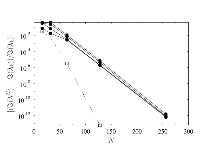
Figure 2: Relative errors in the imaginary parts of the numerically computed eigenvalues $\lambda^{N}$ with respect to the analytical expressions for $\lambda_{k}$ given in equation (31), cf. [7], as a function of the resolution $N$ for vortices with (open symbols) aspect ratio $a/b=4$ and (solid symbols) aspect ratio $a/b=8$. For the aspect ratio $a/b=4$ the eigenmode wavenumber corresponding to the eigenvalue is $k=3$, whereas for the aspect ratio $a/b=8$ the wavenumbers are $k=3,4,5,6$, cf. (34), with larger values of $k$ resulting in larger errors.

6 Conclusions

While perturbation equations similar to (19) have already been used for the linear stability analysis of 2D vortex patches [11, 14, 13], to the best of our knowledge, the present study offers a first complete derivation of this approach. In particular, it relies on methods of the shape calculus which are a general and mathematically consistent way of dealing with the free-boundary aspect of the problem. We add that, in the context of vortex dynamics, such techniques have already been used to study continuation of families of solutions [41] and vortex control problems [49]. The proposed numerical approach is demonstrated to be spectrally-accurate reducing all singular integrals to closed form (24). The two validation tests presented offer “the proof of the concept” for this approach.

Generalization of our method to problems involving several vortices is straightforward, and requires that an equation of the form (19) be written for each individual vortex with the interaction between the vortices captured by the field $U(z)$ (which vanishes identically in the single-vortex examples considered in Sections 3 and 4). This description will be simplified by symmetries of the vortex configuration. One aspect of this problem which does not seem to have received much attention in the literature is the possibility for subcritical disturbance amplification due to non-normality of the underlying stability operator. While these questions have already been investigated for viscous vortices with unbounded vorticity support (e.g., [51, 52]), to the best of our knowledge, there are no results concerning free-boundary problems of the type (1)–(2). Another interesting and far less researched application area for our approach is the stability analysis of 3D axisymmetric vortex flows, with and without swirl, with compact vorticity support [50]. All these problems are left to future research.

As regards limitations of the proposed approach, we remark that shape calculus in its standard formulation [46] is applicable only to problems posed on smooth manifolds, hence our method would need to be modified, so that it can be applied to contours with singularities, such as, e.g., corners (flows with such features typically arise as terminal members of families of steady solutions [41]). Some relevant ideas are already mentioned in [53]. Likewise, analysis of stability with respect to perturbations leading to topology changes requires the use of different methods.

Appendix A Evaluation of the Integral $\int_{0}^{2\pi}\frac{e^{iMq}}{e^{is}-e^{iq}}\,dq$

The calculations presented in Section 3, 4 and 5 required the values of the integrals

$$I=\int_{0}^{2\pi}\frac{e^{iM}}{e^{ip}-e^{iq}}\,dq=e^{-ip}\int_{0}^{2\pi}\frac{e^{iM}}{1-e^{i(q-p)}}\,dq$$ (44)

for integer $M$. If $M>0$, let us consider

$$e^{-ip}\int_{C}\frac{e^{iM}}{1-e^{i(q-p)}}\,dq$$

in which $C$ is now the contour connecting the points $0$, $2\pi$, $2\pi+Yi$, $Yi$, and $0$ with a small semi-circular indentation into the upper half-plane above $p$, where $p$ $\in(0,2\pi)$. This contour integral vanishes by Cauchy’s Theorem. The integrals over the left and right lateral sides of $C$ cancel by periodicity. As regards the top segment of contour $C$, writing $q=x+iY$, we have

$$e^{iMq}=e^{iMx}e^{-MY}\quad\textrm{and}\quad e^{i(q-p)}=e^{i(x-p)}e^{-Y},$$

so for $Y\rightarrow\infty$ the integral over that segment goes to zero. There remains to take the limit of the integral over the bottom segment of the contour $C$ as the radius of the semi-circular indentation vanishes. This is the original principal-value integral (44) augmented by the contribution from the indentation, which can be evaluated using the Cauchy integral formula. To this end, we write the integrand as

$$\frac{e^{iMq}(q-p)}{1-e^{i(q-p)}}\frac{1}{q-p}$$

and find, using L’Hôpital’s rule,

$$\lim_{q\rightarrow p}\frac{e^{iMq}(q-p)}{1-e^{i(q-p)}}=ie^{i(M-1)p}.$$

Thus, the limit of the integral over the indentation is this value multiplied by $-\pi i$, and, finally, we obtain

$$I=\pi i(ie^{i(M-1)p})=-\pi e^{i(M-1)p}.$$ (45)

When $M<1$, instead of contour $C$, we use its reflection into the lower half-plane. Then, since $Y$ is negative, the integral over the bottom segment goes to zero as $Y\rightarrow-\infty$ and, since the small semi circle is positively oriented,

$$I=-\pi i(ie^{i(M-1)p})=\pi e^{i(M-1)p}.$$ (46)

Formulas (45) and (46) are equivalent to (25).

References

- [1] Lord Kelvin, “Vibrations of a columnar vortex”, Phil. Mag 10, 155–168, (1880).
- [2] H. Lamb, Hydrodynamics, Cambridge University press, (1932).
- [3] G. K. Batchelor, An introduction to fluid mechanics, Cambridge University Press, (1967).
- [4] P. G. Saffman, Vortex Dynamics, Cambridge University Press, (1992).
- [5] G. R. Baker, “A Study of the Numerical Stability of the Method of Contour Dynamics”, Phil. Trans. Roy. Soc. 333, 391–400, (1990).
- [6] G. Kirchhoff, Vorlesungen uber Mathematische Physik: Mechanik, Teubner, (1876).
- [7] A. E. H. Love, “On the Stability of certain Vortex Motions”, Proc. London Math. Soc., s1–25, 18-43, (1893).
- [8] D. W. Moore and P. G. Saffman, “Structure of a line vortex in an imposed strain”, in Olsen, Goldburg and Rogers (Eds.) Aircraft wake turbulence, Plenum, 339–354, (1971).
- [9] T. B. Mitchell and L. F. Rossi, “The evolution of Kirchhoff elliptic vortices”, Phys. Fluids 20, 054103 (2008).
- [10] Y. Guo, Ch. Hallstrom, and D. Spirn, “Dynamics Near an Unstable Kirchhoff Ellipse” Commun. Math. Phys. 245, 297–354, (2004).
- [11] D. G. Dritschel, “The stability and energetics of corotating uniform vortices”, J. Fluid Mech. 157, 95–134, (1985).
- [12] D. G. Dritschel, “The stability of elliptical vortices in an external straining flow”, J. Fluid Mech. 210, 223–261, (1990).
- [13] D. G. Dritschel, “A general theory for two–dimensional vortex interactions”, J. Fluid Mech. 293, 269–303, (1995).
- [14] D. G. Dritschel and B. Legras, “The elliptical models of two–dimensional vortex dynamics. II: Disturbance equations”, Phys. Fluids A 3, 855–869, (1991).
- [15] M. R. Dhanak, “Stability of a Regular Polygon of Finite Vortices”, J. Fluid Mech. 234, 297–316, (1992).
- [16] H. M. Wu, E. A. Overman II, and N. J. Zabusky, “Steady–State Solutions of the Euler Equations in Two Dimensions: Rotating and Translating V–States and Limiting Cases. I. Numerical Algorithms and Results”, J. Comp. Phys. 53, 42–71, (1984).
- [17] J. R. Kamm, “Shape and stability of two–dimensional vortex regions”, Ph.D. Thesis, Caltech, (1987).
- [18] A. Elcrat, B. Fornberg B and K. Miller, “Stability of vortices in equilibrium with a cylinder”, J. Fluid Mech. 544, 53–68, (2005).
- [19] J. Burbea, “On Patches of Uniform Vorticity in a Plane of Irrotational Flow”, Arch. Rat. Mech. Anal. 77, 349–358, (1982).
- [20] J. Burbea and M. Landau, “The Kelvin Waves in Vortex Dynamics and Their Stability”, J. Comp. Phys 45, 127–156, (1982).
- [21] B. Turkington, “Corotating Steady Vortex Flows with –Fold Symmetry”, Nonlinear Analysis, Theory, Methods & Applications 9, 351–369, (1985).
- [22] Y. Tang, “Nonlinear Stability of Rankine’s Vortex”, Int. J. Non–Linear Mech. 27, 669–673, (1992).
- [23] Y.-H. Wan, “The Stability of Rotating Vortex Patches”, Commun. Math. Phys. 107, 1–20, (1986).
- [24] Y.-H. Wan, “Bifurcations at Kirchhoff elliptic vortex with eccentricity ”, Dynamics and Stability of Systems” 13, 281–297, (1998).
- [25] P. G. Saffman and R. Szeto, “Equilibrium shapes of a pair of equal uniform vortices”, Phys Fluids 23, 2339–2342, (1980).
- [26] D. G. Dritschel, “Nonlinear stability bounds for inviscid, two-dimensional, parallel or circular flows with monotonic vorticity, and the analogous three- dimensional quasi-geostrophic flows”, J. Fluid Mech. 191, 575–581, (1988).
- [27] C. Cerrtelli and C. H. K. Williamson, “A new family of inform vortices related to vortex configurations before merging”, J. Fluid Mech. 493, 219–229, (2003).
- [28] Y. Fukumoto & H. K. Moffatt, “Kinematic variational principle for motion of vortex rings”, Physica D 237, 2210–2217, (2008).
- [29] P. Luzzatto-Fegiz and C. H. K. Williamson, “Stability of Conservative Flows and New Steady-Fluid Solutions from Bifurcation Diagrams Exploiting Variational Argument”, Phys. Rev. Lett. 104, 044504, (2010).
- [30] P. Luzzatto-Fegiz and C. H. K. Williamson, “Stability of elliptical vortices from imperfect-velocity-impulse diagrams”. Theor. Comput. Fluid Dyn. 24, 181–188, (2010).
- [31] P. Luzzatto-Fegiz and C. H. K. Williamson, “An accurate and efficient method for computing uniform vortices”, J. Comput. Phys. 230, 6495–6511 (2011).
- [32] P. Luzzatto-Fegiz and C. H. K. Williamson,”Resonant instability in two-dimensional vortex arrays”, Proc. R. Soc. A 467, 1164–1185, (2011).
- [33] P. Luzzatto-Fegiz and C. H. K. Williamson, “Structure and stability of the finite-area Kármán street”, Phys. Fluids 24, 066602, (2012).
- [34] P. Luzzatto-Fegiz and C. H. K. Williamson, “Determining the stability of steady two-dimensional flows through imperfect velocity-impulse diagrams”, J. Fluid Mech. 706, 323–350, (2012).
- [35] P. G. Drazin and W. H. Reid, Hydrodynamic Stability, (Second edition), Cambridge University Press, 2004.
- [36] A. J. Majda and A. L. Bertozzi, Vorticity and Incompressible Flow, Cambridge University Press, (2002).
- [37] S. Childress, An Introduction to Theoretical Fluid Mechanics, American Mathematical Society, (2009).
- [38] J.-Z. Wu, H.-Y. Ma and M.-D. Zhou, “Vorticity and Vortex Dynamics”, Springer, (2006).
- [39] B. Turkington, “On Steady vortex flow in two dimensions. Part I”, Comm. in Partial Differential Equations 8, 999–1030, (1983).
- [40] B. Turkington, “On Steady vortex flow in two dimensions. Part II”, Comm. in Partial Differential Equations 8, 1031–1071, (1983).
- [41] F. Gallizio, A. Iollo, B. Protas, and L. Zannetti, “On Continuation of Inviscid Vortex Patches”, Physica D 239, 190–201, (2010).
- [42] J. Sokolowski and J.-P. Zolésio, Introduction to shape optimization: shape sensitivity analysis, Springer, (1992).
- [43] M. C. Delfour and J.-P. Zolésio, “Shape and Geometries — Analysis, Differential Calculus and Optimization”, SIAM, (2001).
- [44] J. Haslinger and R. A. E. Mäkinen, Introduction to Shape Optimization: Theory, Approximation and Computation, SIAM, (2003).
- [45] S. Schmidt and V. Schulz, “Shape derivatives for general objective functions and the incompressible Navier–Stokes equations”, Control and Cybernetics 39, 677–713, (2010).
- [46] M. C. Delfour and J.-P. Zolésio, “Dynamical free boundary problem for an incompressible potential fluid flow in a time-varying domain”, Journal of Ill-Posed and Inverse Problems 1, 1–25, (2004).
- [47] D. Pullin, ”The nonlinear behavior of a constant vorticity layer at a wall”, J. Fluid Mech.108, 401-412, (1981).
- [48] W. Hackbusch, “Integral Equations: Theory and Numerical Treatment”, Birkhäuser, (1995).
- [49] B. Protas, “Vortex Design Problem”, Journal of Computational and Applied Mathematics 236, 1926–1946, 2012.
- [50] A. Elcrat, B. Fornberg, and K. Miller, “Steady axisymmetric vortex flows with swirl and shear”, J. Fluid Mechanics 613, 395–410, (2008).
- [51] D. S. Pradeep And F. Hussain, “Transient growth of perturbations in a vortex column”, Journal of Fluid Mechanics 550, 251–288, (2006).
- [52] X. Mao, S. J. Sherwin and H. M. Blackburn, “Non-normal dynamics of time-evolving co-rotating vortex pairs” Journal of Fluid Mechanics 701, 430–459, (2012).
- [53] A. Elcrat and K. G. Miller, “Variational Formulas on Lipshitz Domains”, Transactions of the AMS 347, 2669–2678 (1995).