A Learning Framework for Morphological Operators using Counter–Harmonic Mean

Abstract

We present a novel framework for learning morphological operators using counter-harmonic mean. It combines concepts from morphology and convolutional neural networks. A thorough experimental validation analyzes basic morphological operators dilation and erosion, opening and closing, as well as the much more complex top-hat transform, for which we report a real-world application from the steel industry. Using online learning and stochastic gradient descent, our system learns both the structuring element and the composition of operators. It scales well to large datasets and online settings.

1 Introduction

Mathematical morphology (MM) is a nonlinear image processing methodology based on computing max/min filters in local neighborhoods defined by structuring elements [16, 17]. By concatenation of two basic operators, i.e., the dilation $\delta_{B}(f)$ and the erosion $\varepsilon_{B}(f)$, on the image $f$, we obtain the closing $\varphi_{B}(f)=\varepsilon_{B}\left(\delta_{B}(f)\right)$ and the opening $\varphi_{B}(f)=\gamma_{B}\left(\delta_{B}(f)\right)$, which are filters with scale-space properties and selective feature extraction skills according to the underlaying structuring element $B$. Other more sophisticated filters are obtained by combinations of openings and closings, to address problems such as non-Gaussian denoising, image regularization, etc.

Finding the proper pipeline of morphological operators and structuring elements in real applications is a cumbersome and time consuming task. In the machine learning community there has always been lot of interest in learning such operators, but due to the non-differentiable nature of the max/min filtering only few approaches have been found to succeed, notably one based on LMS (gradient steepest descent algorithm) for rank filters formulated with the sign function [13, 14]. This idea was later revisited [12] in a neural network framework combining morphological/rank filters and linear FIR filters. Other attempts from the evolutionary community (e.g., genetic algorithms [7] or simulated annealing [21]) use black-box optimizers to circumvent the differentiability issue. However, most of the proposed approaches do not cover all operators. More importantly, they cannot learn both the structuring element and the operator, e.g.,  [11]. This is obviously a quite important limitation as it makes very hard or even impossible the composition of complex filtering pipelines. Furthermore, such systems are usually limited to a very specific application and hardly generalize to complex scenarios.

Inspired by recent work [1] on counter-harmonic mean asymptotic morphology, we propose a novel framework to learn morphological pipelines of operators. We combine convolutional neural networks (CNN) with a new type of layer that permits complex pipelines through multiple layers and therefore extends this models to a Morphological Convolutional Neural Network (MPCNN). It extends previous work on deep-learning while making directly applicable all optimization tricks and findings of this field.

Here we focus on methodological foundations and show how the model learns several operator pipelines, from dilation/erosion to top-hat transform (i.e., residue of opening/closing). We report an important real-world application from the steel industry, and present a sample application to denoising where operator learning outperforms hand-crafted structuring elements.

Our main contributions are:

• a novel framework where learning of morphological operators and filtering pipelines can be performed using gradient-based techniques, exploiting recent insights of deep-learning approaches;

• the introduction of a novel PConv layer for CNN, to let CNN benefit from highly nonlinear, morphology-based filters;

• the stacking of many PConv layers, to learn complex pipelines of operators such as opening, closing and top-hats.

2 Background

Here we illustrate the foundations of our approach, introducing the Counter-Harmonic Mean formulation for asymptotic morphology and CNN.

2.1 Asymptotic morphology using Counter-Harmonic Mean

We start from the notion of counter-harmonic mean [2], initially used  [19] for constructing robust morphological-like operators. More recently, its morphological asymptotic behavior was characterized [1]. Let $f(x)$ be a 2D real-valued image, i.e., $f:\Omega\subset\mathbb{Z}^{2}\rightarrow\mathbb{R}$, where $x\in\Omega$ denotes the coordinates of the pixel in the image domain $\Omega$. Given a (positive) weighting kernel $w:W\rightarrow\mathbb{R}_{+}$, $W$ being the support window of the filter, the counter-harmonic mean (CHM) filter of order $P$, $-\infty\leq P\leq\infty$ is defined by,

$$\kappa_{w}^{P}(f)(x)=\frac{(f^{P+1}\ast w)(x)}{(f^{P}\ast w)(x)}=\frac{\int_{y\in W(x)}f^{P+1}(y)w(x-y)dy}{\int_{y\in W(x)}f^{P}(y)w(x-y)dy},$$ (1)

where $f^{P}$ is the image, where each pixel value of $f$ is raised to power $P$, $/$ indicates pixel-wise division, and $W(y)$ is the support window of the filter $w$ centered on point $y$. We note that the CHM filter can be interpreted as $P-$deformed convolution, i.e., $\kappa_{w}^{P}(f)(x)\equiv(f\ast_{P}w)(x)$. For $P\gg 0$ ($P\ll 0$) the pixels with largest (smallest) values in the local neighborhood $W$ will dominate the result of the weighted sum (convolution), therefore morphological dilation and erosion are the limit cases of the CHM filter, i.e., $\lim_{P\rightarrow+\infty}(f\ast_{P}w)(x)=$ $\sup_{y\in W(x)}f(y)=$ $\delta_{W}(f)(x)$, and $\lim_{P\rightarrow-\infty}(f\ast_{P}w)(x)=$ $\inf_{y\in W(x)}f(y)=$ $\varepsilon_{W}(f)(x)$, where $W$ plays the role of the structuring element. As proven earlier [1], apart from the limit cases (e.g., a typical order of magnitude of $5\leq|P|<10$), we have the following behavior:

$$(f\ast_{P}w)(x)\mid_{P\gg 0} \approx \sup_{y\in W(x)}\left\{f(\mathbf{y})+\frac{1}{P}\log\left(w(x-y)\right)\right\},$$ (2)

$$(f\ast_{P}w)(x)\mid_{P\ll 0} \approx \inf_{y\in W(x)}\left\{f(\mathbf{y})-\frac{1}{P}\log\left(w(x-y)\right)\right\},$$ (3)

which can be interpreted, respectively, as the nonflat dilation (supremal convolution) and nonflat erosion (infimal convolution) using the structuring function $b(x)=\frac{1}{P}\log\left(w(x)\right)$. By using constant weight kernels, i.e., $w(x)=1$ if $x\in W$ and $w(x)=0$ if $x\notin W$, and $|P|\gg 0$, we just recover the corresponding flat structuring element $W$, associated to the structuring function $\mathfrak{w}(x)=0$ if $x\in W$ and $\mathfrak{w}(x)=-\infty$ if $x\notin W$.

From a precise morphological viewpoint, we notice that for finite $P$ one cannot guarantee that $(f\ast_{P}w)(x)$ yields exactly a pair of dilation/erosion, in the sense of commutation with max/min [16, 17]. Consequently, stricto sensu, we can only name them as pseudo-dilation ($P\gg 0$) and pseudo-erosion ($P\ll 0$). The asymptotic cases of the CHM filter can be also combined to approximate opening and closing operators, i.e.,

$$\left\{\begin{array}[]{lll}\left((f\ast_{-P}w)\ast_{P}w\right)(x)&\xrightarrow{P\gg 0}&\gamma_{W}(f)(x),\\ \left((f\ast_{P}w)\ast_{-P}w\right)(x)&\xrightarrow{P\ll 0}&\varphi_{W}(f)(x).\end{array}\right.$$ (4)

2.2 Convolutional Neural Networks

CNN are hierarchical models alternating two basic operations, convolution and subsampling, reminiscent of simple and complex cells in the primary visual cortex [8]. Their main characteristic is that they exploit the 2D structure of images via weight sharing, learning a set of convolutional filters. Certain CNN scale well to real-sized images and excel in many object recognition [3, 4, 6, 10] and segmentation [5, 18] benchmarks. We refer to a state-of-the-art CNN as depicted in Figure 1. It consists of several basic building blocks briefly explained here:

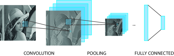
Figure 1: A schematic representation of an CNN. Convolutional and pooling layers are stacked below the fully connected layers used for classification.

• Convolutional Layer: performs a 2D filtering between input images $\left\{f_{i}\right\}_{i\in I}$ and a bank of filters $\left\{w_{k}\right\}_{k\in K}$, producing another set of images $\left\{h_{j}\right\}_{j\in J}$ denoted as maps. Input-output correspondences are specified through a connection table $CT$ (inputImage $i$, filterId $k$, outputImage $j$). Filter responses from inputs connected to the same output image are linearly combined. This layer performs the following mapping: $h_{j}(x)=\sum_{i,k\in CT_{i,k,j}}(f_{i}\ast w_{k})(x),$ where $\ast$ indicates the 2D valid convolution. Then, a nonlinear activation function (e.g., $tanh$, $logistic$, etc.) is applied to $h_{j}$. Recently $relu$ activations have been found to excel. They are the units we use for all our models. A $relu$ unit operates as $relu(x)=\max(lb,\min(x,ub))$. It is common choice to use $0$ as lower bound ($lb$) and $\infty$ as upper bound ($ub$).

• Pooling Layer: down-samples the input images by a constant factor keeping a value (e.g. maximum or average) for every non overlapping subregion of size $p$ in the images. Max-Pooling is generally favorable, as it introduces small invariance to translation and distortion, leads to faster convergence and better generalization [15].

• Fully Connected Layer: this is the standard layer of a multi-layer network. It performs a linear multiplication of the input vector by a weight matrix.

Note the striking similarity between the max-pooling layer and a dilation transform. The former is in fact a special case of dilation, with a square structuring element of size $p$ followed by downsampling (sampling one out of every $p$ pixels). Our novel layer, however, does not any longer limit the pooling operation to simple squares, but allows for a much richer repertoire of structuring elements fine-tuned for given tasks. This is what makes MCNN so powerful.

3 Method

Now we are ready to introduce the novel morphological layer based on CHM filter formulation, referred to as PConv layer. For a single channel image $f(x)$ and a single filter $w(x)$ the PConv layer performs the following operation

$$PConv(f;w,P)(x)=\frac{(f^{P+1}\ast w)(x)}{(f^{P}\ast w)(x)}=(f\ast_{P}w)(x)$$ (5)

It is parametrized by $P$, a scalar which controls the type of operation ($P<0$ pseudo-erosion, $P>0$ pseudo-dilation and $P=0$ standard linear convolution), and by the weighting kernel $w(x)$, where the corresponding asymptotic structuring function is given by $\mathfrak{w}(x)=\log\left(w(x)\right)$. Since this formulation is differentiable we can use gradient descent on these parameters.

The gradient of such a layer is computed by back-propagation [20, 9]. In minimizing a given objective function $L(\theta;X)$, where $\theta$ represents the set of parameters in the model, back-propagation applies the chain rule of derivatives to propagate the gradients down to the input layer, multiplying them by the Jacobian matrices of the traversed layers. Let us introduce first two partial results of back-propagation

$$\Delta_{U}(x)=\frac{f(x)}{(f^{P}\ast w)(x)};\quad\Delta_{D}(x)=\frac{-f(x)\cdot(f^{P+1}\ast w)(x)}{(f^{P}\ast w)(x)}.$$ (6)

The gradient of a PConv layer is computed as follows

$$\frac{\partial L}{\partial w} = \tilde{f}^{P+1}*\Delta_{U}+\tilde{f}^{P}\ast\Delta_{D}$$ (7)

$$\frac{\partial L}{\partial P} = f^{P+1}\cdot\log(f)\cdot(\frac{f}{f^{P}\ast w}\ast\tilde{w})+f^{P}\cdot\log(f)\cdot(\Delta_{D}\ast\tilde{w})$$ (8)

where $\tilde{f},\tilde{w}$ indicate flipping along the two dimensions and $\cdot$ indicates element-wise multiplication. The partial derivative of the PConv layer with respect to its input (to back-propagate the gradient) is instead

$$\frac{\partial(f\ast_{P}w)(x)}{\partial f}=\Delta_{U}(x)+\Delta_{D}(x).$$ (9)

Learning the top-hat operator requires a short-circuit in the network to allow for subtracting the input image (or the result of an intermediate layer) from the output of a filtering chain. For this purpose we introduce the AbsDiffLayer which takes two layers as input and emits the absolute difference between them. Partial derivatives can still be back-propagated.

3.1 Learning Algorithm

Minimizing a PConv layer is a non-convex, highly non-linear operation prone to local convergence. Deep-learning findings tell us that stochastic gradient descent is the most effective algorithm to train such complex models. In our experiments we use its full online version where weights are updated sample by sample. The learning rate decays during training. To further avoid bad local minima we use a momentum term. For the opening/closing tasks we also alternate between learning $P$, keeping $w$ fixed, and vice-versa. This is common in online dictionary learning and sparse coding. We also constrain $w\geq 0$.

4 Experiments

We thoroughly evaluate our MCNN on several tasks. First we assess the quality of dilation/erosion operators, which require a single PConv layer. This gives a good measure of how well training can be performed using the CHM derivation. Then we investigate a two-layer network learning openings/closings. This is already a challenging task hardly covered in previous approaches.

We then learn the top-hat transform for a very challenging steel industry application. Using $2$ filters per layer we learn to simultaneously detect two families of defects without resorting to multiple training. Our implementation allows for learning multiple filters for every layer, thus producing a very rich set of filtered maps. Subsequent convolutional layers can learn highly nonlinear embeddings. (We believe that this will also dramatically improve segmentation capabilities of such models to be investigated in future work.) We also show that a simple CNN does not learn well pipelines of morphological operators. This is actually expected a priori due to the nature of conventional convolutional layers, and shows the value of our novel PConv layer.

As final benchmark we consider denoising. Our MCNN shows the superiority of operator learning over hand-crafting structuring elements for non-Gaussian (binomial and salt-and-pepper) noise. We also show that our approach performs well on total variation (TV) approximation for additive Gaussian noise.

In all our experiments we use stochastic gradient descent and a filter size of $11\times 11$ unless otherwise stated. The per-pixel mean-squared error loss (MSE) is used.

4.1 Learning dilation and erosion

In this first set of experiments we create a dataset as follows: for every input image $f_{i}$ we produce a target image $t_{j}$ using a predetermined flat structuring element $B_{k}$ and a predetermined operator: $t_{j}=\delta_{B_{k}}(f_{i})$ or $t_{j}=\varepsilon_{B_{k}}(f_{i})$. We train until convergence. Overfitting is not an issue in such a scenario. The net actually learns the true function underlying the data. In fact, for an image of $512\times 512$ and a structuring element with support of $11\times 11$ there are $502^{2}$ patches, way more than the $11^{2}$ elements in the structuring element. A CNN with equal topology fails, producing mainly Gaussian blurred images, illustrating the need for a PConv layer to handle this kind of nonlinearities. Figure 2 shows the results of a dilation with three structuring elements: a line of $15$ pixels and $45^{\circ}$, a square of size $5$ pixels and a diamond of side $5$ pixels. Figure 3 shows similar results for the erosion transform.

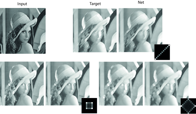
Figure 2: Examples of learning a dilation with three different structuring elements. The target and net output are slightly smaller than the original image due to valid convolution. The obtained kernel $w(x)$ for each case is also depicted.

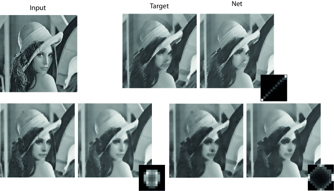
Figure 3: Examples of learning an erosion with three different structuring elements along with the learned kernel $w(x)$.

Note that the learned weighted kernels $w(x)$ are not exactly uniformly equal to $1$. The corresponding morphological structuring function $\mathfrak{w}(x)$, obtained after applying the logarithm on the weights, produces a rather flat shape. In practice, we observed that learning an erosion is slightly more difficult than learning the dual dilation. This is related to the asymmetric numerical behavior of CHM for $P>0$ and $P<0$. Nevertheless, in all cases the learned operator has excellent performance.

4.2 Learning opening and closing

In this set of experiments we train our system to learn openings $\gamma_{B_{k}}(f_{i})$ and closings $\varphi_{B_{k}}(f_{i})$. Learning such functions is extremely difficult. To the best of our knowledge, we are the first to do this in a flexible and gradient-based framework without any prior. For instance, in classical approaches [13] or more recent ones [11], the operator needs to be fixed a priori.

Figure 4-top shows an example of a closing with a line of length $10$ and an orientation of $45^{\circ}$, whereas Figure 4-bottom shows an example of an opening with a square of size $5$. In both cases, the obtained kernel for the first $L1$ and second $L2$ PConv layers are depicted. We see that the associated structuring element is learned with a good approximation. On the other hand, however, we also start to see that learning a flat opening/closing is remarkably hard and that the network output starts to be slightly “blurry”. Why? On the one hand, the obtained values of $P$, e.g., in the closing $P_{L1}=6.80$ and $P_{L2}=-8.85$, in the opening $P_{L1}=-7.64$ and $P_{L2}=7.07$ are in the interval of asymptotically unflat behavior. On the other hand, they are not totally symmetric. We intend to further study these issues in ongoing work.

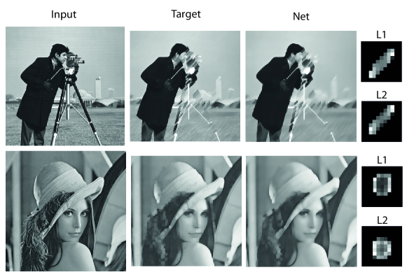
Figure 4: Top: an example of learning a closing operator where a line of length $10$ and orientation $45^{\circ}$ is used. Bottom: opening with a square structuring element of size $5$. The network closely matches the output and almost perfectly learns the structuring elements in both PConv layers.

4.3 Learning top-hat transform

Delegating the learning to a neural network allows for easily constructing complex topologies by linking several simple modules. We recall that the white top-hat is the residue of the opening, i.e., $\varrho^{+}_{B_{k}}(f_{i})=f_{i}-\gamma_{B_{k}}(f_{i})$, and the black top-that the residue of the closing, i.e., $\varrho^{-}_{B_{k}}(f_{i})=\varphi_{B_{k}}(f_{i})-f_{i}$. Thus, to learn a top-hat transform we introduce the AbsDiff layer. It takes two layers as input and emits their absolute difference in output. Backpropagation is performed as usual.

Top-hat is particularly relevant in real applications such as steel surface quality control. It is a powerful tool for defect detection. Here we first show that our framework can learn such a transform. Increasing the number of filters per layer from $1$ to $2$, we show that our MCNN is also much more powerful when jointly learning two transforms.

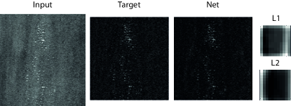
Figure 5: Learning a top-hat transform. The defected input image has bright spots to be detected. The network performs almost perfectly on this challenging task.

Figure 5 shows the results for a single top-hat. We create our training set by applying a white top-hat $\varrho^{+}_{B}$, where $B$ is a disk of size $5$ pixels. This operator extracts only the structures of size smaller than $B$ and brighter than the background. We clearly see that the network performs almost perfectly. To further assess the advantages of a PConv layer over a conventional convolutional layer, we also train a CNN with identical topology. The discrepancy between the two models in terms of losses (MSE) is large: we have 1.28E-3 for our MCNN and 1.90E-3 for the CNN. More parameters are required for a CNN to reach better performance. This clearly establishes the added value of our MCNN.

The steel industry requires many top-hat operations. Tuning them one by one is a cumbersome process. Furthermore, several models’ outputs need to be considered to obtain the final detection result. Figure 6 shows that by simply increasing the number of filters per layer we can simultaneously learn two top-hat transforms and address this problem. We learn a white top-hat with a disk of size $5$ and a black top-hat with a line of size $10$ and orientation of $0^{\circ}$. A convolutional layer is used to combine the output of the two operators. The architecture is as follows: 2 PConv layers, Conv layer, AbsDiff layer with the input. The network is almost perfect from our viewpoint. This opens the possibility of using such a setup in more complex scenarios where several morphological operators should be combined. This is of great interest in multiple class steel defect detection.

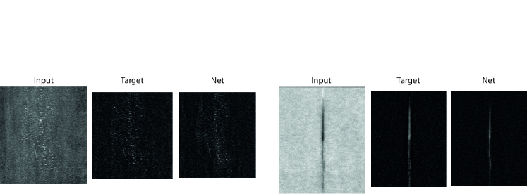
Figure 6: Learning two top-hat transforms. On the left, bright spots need to be detected. On the right, a dark vertical line. The network performs almost perfectly in this challenging task.

4.4 Learning denoising and image regularization

Finally we compare our MCNN to conventional morphological pipelines in the denoising task. Morphological filters are recommended for non-Gaussian denoising. The purpose of this evaluation, however, is not to propose a novel noise removal approach, but to show the advantages of a learnable pipeline over a hand-crafted one.

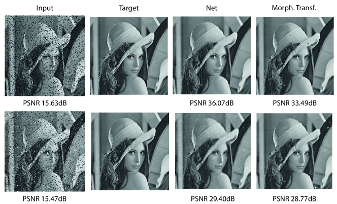
Figure 7: Top: Binomial noise removal task. The learned nonlinear operator performs better than the hand-crafted one. Learning uses noisy and original images—there is no prior on the task. Bottom: Salt’n’pepper noise removal task. Even here, the learned operator performs better than the corresponding morphological one.

We start with binomial noise where $10$% of the image pixels are switched-off. The topology in this case is: $2$ PConv layers and filter size of $5\times 5$. We compare to a closing with a square of size $2$, empirically found to deliver best results. We make the task even harder by using larger-than-optimal support. Training is performed in fully on-line fashion. While the target images are kept fixed, the input is generated by adding random noise sample by sample. So the network never sees the same pattern twice. Figure 7–top compares the two approaches, and shows the noisy image. We see that learning substantially improves the PSNR measure.

We continue with an even more challenging task, a $10\%$ salt’n’pepper denoising. The network is made of $4$ PConv layers, a very long pipeline. We compare to an opening with a square of size $2\times 2$ on a closing with the same structuring element. Training follows the same protocol as the one for the binomial noise. Images are generated online. This creates a possibly infinite dataset with very small memory footprint. Figure 7–bottom shows results. Although we can observe some limitations of our approach, it still exhibits the best PSNR also in this application.

Finally we consider the case of total variation (TV) restoration from an image corrupted by $6$% additive Gaussian noise. Morphological filtering does not excel at this task. A MCNN is trained to learn the mapping from noisy image to TV restored image. How well can it approximate any target transformation with a pseudo-morphological pipeline? The architecture is composed of $2$ PConv layers with $2$ filters each plus an averaging layer. Results are shown in Figure 8.

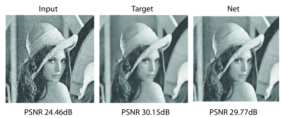
Figure 8: Total Variation (TV) task. The network has to learn to approximate the TV output (target) by means of averaging two filtering pipelines.

5 Conclusion and Perspectives

Our MCNN for learning morphological operators is based on a novel PConv convolutional layer and inherits all the benefits of gradient-based deep-learning algorithms. It can easily learn complex topologies and operator chains such as white/black top-hats and we showed its application to steel defect detection. In future work we intend to let MCNN simultaneously learn banks of morphological filters and longer filtering pipelines.

References

- [1] Angulo, J.: Pseudo-morphological image diffusion using the counter-harmonic paradigm. In: Proc. of ACIVS’2010, LNCS Vol. 6474, Part I. pp. 426–437. Springer (2010)
- [2] Bullen, P.: Handbook of Means and Their Inequalities, 2nd Edition. Springer (1987)
- [3] Cireşan, D.C., Meier, U., Masci, J., Schmidhuber, J.: A committee of neural networks for traffic sign classification. In: International Joint Conference on Neural Networks (IJCNN2011) (2011)
- [4] Cireşan, D.C., Meier, U., Masci, J., Schmidhuber, J.: Flexible, high performance convolutional neural networks for image classification. In: International Joint Conference on Artificial Intelligence (IJCAI2011) (2011)
- [5] Ciresan, D.C., Giusti, A., Gambardella, L.M., Schmidhuber, J.: Deep neural networks segment neuronal membranes in electron microscopy images. In: NIPS (2012)
- [6] Ciresan, D.C., Meier, U., Gambardella, L.M., Schmidhuber, J.: Convolutional neural network committees for handwritten character classification. In: ICDAR. pp. 1250–1254 (2011)
- [7] Harvey, N.R., Marshall, S.: The use of genetic algorithms in morphological filter design. Signal Processing: Image Communication 8(1), 55–71 (1996)
- [8] Hubel, D.H., Wiesel, T.N.: Receptive fields and functional architecture of monkey striate cortex. The Journal of physiology 195(1), 215–243 (March 1968)
- [9] LeCun, Y.: Une procédure d’apprentissage pour réseau à seuil asymétrique. Proceedings of Cognitiva 85, Paris pp. 599–604 (1985)
- [10] Masci, J., Meier, U., Cireşan, D.C., G., F., Schmidhuber, J.: Steel defect classification with max-pooling convolutional neural networks. In: International Joint Conference on Neural Networks (2012)
- [11] Nakashizuka, M., Takenaka, S., Iiguni, Y.: Learning of structuring elements for morphological image model with a sparsity prior. In: IEEE International Conference on Image Processing, ICIP 2010. pp. 85–88 (2010)
- [12] Pessoa, L.F.C., Maragos, P.: Mrl-filters: a general class of nonlinear systems and their optimal design for image processing. IEEE Transactions on Image Processing 7(7), 966–978 (1998)
- [13] Salembier, P.: Adaptive rank order based filters. Signal Processing 27, 1–25 (1992)
- [14] Salembier, P.: Structuring element adaptation for morphological filters. J. of Visual Communication and Image Representation 3(2), 115–136 (1992)
- [15] Scherer, D., Müller, A., Behnke, S.: Evaluation of pooling operations in convolutional architectures for object recognition. In: International Conference on Artificial Neural Networks (2010)
- [16] Serra, J.: Image analysis and mathematical morphology. Academic Press, London (1982)
- [17] Soille, P.: Morphological Image Analysis: Principles and Applications. Springer-Verlag Berlin (1999)
- [18] Turaga, S.C., Murray, J.F., Jain, V., Roth, F., Helmstaedter, M., Briggman, K., Denk, W., Seung, H.S.: Convolutional networks can learn to generate affinity graphs for image segmentation. Neural Comput. 22(2), 511–538 (Feb 2010)
- [19] Vliet, L.J.v.: Robust local max-min filters by normalized power-weighted filtering. In: Proc. of IEEE ICPR’04, Vol. 1. pp. 696–699 (2004)
- [20] Werbos, P.J.: Beyond Regression: New Tools for Prediction and Analysis in the Behavioral Sciences. Ph.D. thesis, Harvard University (1974)
- [21] Wilson, S.S.: Training structuring elements in morphological networks. In: Mathematical Morphology in Image Processing, Chapter 1, pp. 1–42. Marcel Dekker (1993)