Efficient moment-based inference of admixture parameters and sources of gene flow

Abstract

The recent explosion in available genetic data has led to significant advances in understanding the demographic histories of and relationships among human populations. It is still a challenge, however, to infer reliable parameter values for complicated models involving many populations. Here we present MixMapper, an efficient, interactive method for constructing phylogenetic trees including admixture events using single nucleotide polymorphism (SNP) genotype data. MixMapper implements a novel two-phase approach to admixture inference using moment statistics, first building an unadmixed scaffold tree and then adding admixed populations by solving systems of equations that express allele frequency divergences in terms of mixture parameters. Importantly, all features of the model, including topology, sources of gene flow, branch lengths, and mixture proportions, are optimized automatically from the data and include estimates of statistical uncertainty. MixMapper also uses a new method to express branch lengths in easily interpretable drift units. We apply MixMapper to recently published data for HGDP individuals genotyped on a SNP array designed especially for use in population genetics studies, obtaining confident results for 30 populations, 20 of them admixed. Notably, we confirm a signal of ancient admixture in European populations—including previously undetected admixture in Sardinians and Basques—involving a proportion of 20–40% ancient northern Eurasian ancestry.

Introduction

The most basic way to represent the evolutionary history of a set of species or populations is through a phylogenetic tree, a model that in its strict sense assumes that there is no gene flow between populations after they have diverged (?). In many settings, however, groups that have split from one another can still exchange genetic material. This is certainly the case for human population history, during the course of which populations have often diverged only incompletely or diverged and subsequently mixed again (???????). To capture these more complicated relationships, previous studies have considered models allowing for continuous migration among populations (???) or have extended simple phylogenetic trees into admixture trees, in which populations on separate branches are allowed to re-merge and form an admixed offspring population (?????). Both of these frameworks, of course, still represent substantial simplifications of true population histories, but they can help capture a range of new and interesting phenomena.

Several approaches have previously been used to build phylogenetic trees incorporating admixture events from genetic data. First, likelihood methods (???) use a full probabilistic evolutionary model, which allows a high level of precision with the disadvantage of greatly increased computational cost. Consequently, likelihood methods can in practice only accommodate a small number of populations (????). Moreover, the tree topology must generally be specified in advance, meaning that only parameter values can be inferred automatically and not the arrangement of populations in the tree. By contrast, the moment-based methods of ? and ? use only means and variances of allele frequency divergences. Moments are simpler conceptually and especially computationally, and they allow for more flexibility in model conditions. Their disadvantages can include reduced statistical power and difficulties in designing precise estimators with desirable statistical properties (e.g., unbiasedness) (?). Finally, a number of studies have considered “phylogenetic networks,” which generalize trees to include cycles and multiple edges between pairs of nodes and can be used to model population histories involving hybridization (??). However, these methods also tend to be computationally expensive.

In this work, we introduce MixMapper, a new computational tool that fits admixture trees by solving systems of moment equations involving the pairwise distance statistic $f_{2}$ (??), which is the average squared allele frequency difference between two populations. The theoretical expectation of $f_{2}$ can be calculated in terms of branch lengths and mixture fractions of an admixture tree and then compared to empirical data. MixMapper can be thought of as a generalization of the qpgraph package (?), which takes as input genotype data, along with a proposed arrangement of admixed and unadmixed populations, and returns branch lengths and mixture fractions that produce the best fit to allele frequency moment statistics measured on the data. MixMapper, by contrast, performs the fitting in two stages, first constructing an unadmixed scaffold tree via neighbor-joining and then automatically optimizing the placement of admixed populations onto this initial tree. Thus, no topological relationships among populations need to be specified in advance.

Our method is similar in spirit to the independently developed TreeMix package (?). Like MixMapper, TreeMix builds admixture trees from second moments of allele frequency divergences, although it does so via a composite likelihood maximization approach made tractable with a multivariate normal approximation. Procedurally, TreeMix initially fits a full set of populations as an unadmixed tree, and gene flow edges are added sequentially to account for the greatest errors in the fit (?). This format makes TreeMix well-suited to handling very large trees: the entire fitting process is automated and can include arbitrarily many admixture events simultaneously. In contrast, MixMapper begins with a carefully screened unadmixed scaffold tree to which admixed populations are added with best-fitting parameter values, an interactive design that enables precise modeling of particular populations of interest.

We use MixMapper to model the ancestral relationships among 52 populations from the CEPH-Human Genome Diversity Cell Line Panel (HGDP) (??) using recently published data from a new, specially ascertained SNP array designed for population genetics applications (??). Previous studies of these populations have built simple phylogenetic trees (??), identified a substantial number of admixed populations with likely ancestors (?), and constructed a large-scale admixture tree (?). Here, we add an additional level of quantitative detail, obtaining best-fit admixture parameters with bootstrap error estimates for 30 HGDP populations, of which 20 are admixed. The results include, most notably, a significant admixture event (?) in the history of all sampled European populations, among them Sardinians and Basques.

New Approaches

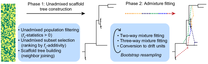
Figure 1: MixMapper workflow. MixMapper takes as input an array of SNP calls annotated with the population to which each individual belongs. The method then proceeds in two phases, first building a tree of (approximately) unadmixed populations and then attempting to fit the remaining populations as admixtures. In the first phase, MixMapper produces a ranking of possible unadmixed trees in order of deviation from $f_{2}$-additivity; based on this list, the user selects a tree to use as a scaffold. In the second phase, MixMapper tries to fit remaining populations as two- or three-way mixtures between branches of the unadmixed tree. In each case MixMapper produces an ensemble of predictions via bootstrap resampling, enabling confidence estimation for inferred results.

The central problem we consider is: given an array of SNP data sampled from a set of individuals grouped by population, what can we infer about the admixture histories of these populations using simple statistics that are functions of their allele frequencies? Methodologically, the MixMapper workflow (Figure 1) proceeds as follows. We begin by computing $f_{2}$ distances between all pairs of study populations, from which we construct an unadmixed phylogenetic subtree to serve as a scaffold for subsequent mixture fitting. The choice of populations for the scaffold is done via initial filtering of populations that are clearly admixed according to the 3-population test (??), followed by selection of a subtree that is approximately additive along its branches, as is expected in the absence of admixture (see Material and Methods and Text S1 for full details).

Next, we expand the model to incorporate admixtures by attempting to fit each population not in the scaffold as a mixture between some pair of branches of the scaffold. Putative admixtures imply algebraic relations among $f_{2}$ statistics, which we test for consistency with the data, allowing us to identify likely sources of gene flow and estimate mixture parameters (Figure 2; Text S1). After determining likely two-way admixture events, we further attempt to fit remaining populations as three-way mixtures involving the inferred two-way mixed populations, by similar means. Finally, we use a new formula to convert the $f_{2}$ tree distances into absolute drift units (Text S2). Importantly, we apply a bootstrap resampling scheme (??) to obtain ensembles of predictions, rather than single values, for all model variables. This procedure allows us to determine confidence intervals for parameter estimates and guard against overfitting. For a data set on the scale of the HGDP, after initial setup time on the order of an hour, MixMapper determines the best-fit admixture model for a chosen population in a few seconds, enabling real-time interactive investigation.

Results

Simulations

To test the inference capabilities of MixMapper on populations with known histories, we ran it on two data sets generated with the coalescent simulator ms (?) and designed to have similar parameters to our human data. In both cases, we simulated 500 regions of 500 kb each for 25 diploid individuals per population, with an effective population size of 5,000 or 10,000 per population, a mutation rate of $0.5\times 10^{-8}$ per base per generation (intentionally low so as not to create unreasonably many SNPs), and a recombination rate of $10^{-8}$ per base per generation. Full ms commands can be found in Material and Methods. We ascertained SNPs present at minor allele frequency 0.05 or greater in an outgroup population and then removed that population from the analysis.

For the first admixture tree, we simulated six non-outgroup populations, with one of them, pop6, admixed (Figure 3A). Applying MixMapper, no admixtures were detected with the 3-population test, but the most additive subset with at least five populations excluded pop6 (max deviation from additivity $2.0\times 10^{-4}$ versus second-best $7.7\times 10^{-4}$; see Material and Methods), so we used this subset as the scaffold tree. We then fit pop6 as admixed, and MixMapper recovered the correct gene flow topology with 100% confidence and inferred the other parameters of the model quite accurately (Figure 3B; Table S1). For comparison, we also analyzed the same data with TreeMix and again obtained accurate results (Figure 3C).

For the second test, we simulated a complex admixture scenario involving 10 non-outgroup populations, with six unadmixed and four admixed (Figure 3D). In this example, pop4 is recently admixed between pop3 and pop5, but over a continuous period of 40 generations. Meanwhile, pop8, pop9, and pop10 are all descended from older admixture events, which are similar but with small variations (lower mixture fraction in pop9, 40-generation continuous gene flow in pop10, and subsequent pop2-related admixture into pop8). In the first phase of MixMapper, the recently admixed pop4 and pop8 were detected with the 3-population test. From among the other eight populations, a scaffold tree consisting of pop1, pop2, pop3, pop5, pop6, and pop7 provided thorough coverage of the data set and was more additive (max deviation $3.5\times 10^{-4}$) than the secon-best six-population scaffold ($5.4\times 10^{-4}$) and the best seven-population scaffold ($1.2\times 10^{-3}$). Using this scaffold, MixMapper returned very accurate and high-confidence fits for the remaining populations (Figure 3E; Table S1), with the correct gene flow topologies inferred with 100% confidence for pop4 and pop10, 98% confidence for pop9, and 61% confidence for pop8 (fit as a three-way admixture; 39% of replicates placed the third gene flow source on the branch adjacent to pop2, as shown in Table S1). In contrast, TreeMix inferred a less accurate admixture model for this data set (Figure 3F). TreeMix correctly identified pop4 as admixed, and it placed three migration edges among pop7, pop8, pop9, and pop10, but two of the five total admixtures (those originating from the common ancestor of pops 3–5 and the common ancestor of pops 9–10) did not correspond to true events. Also, TreeMix did not detect the presence of admixture in pop9 or the pop2-related admixture in pop8.

Application of MixMapper to HGDP data

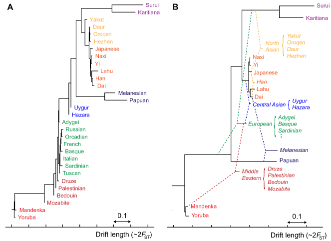
Figure 4: Aggregate phylogenetic trees of HGDP populations with and without admixture. (A) A simple neighbor-joining tree on the 30 populations for which MixMapper produced high-confidence results. This tree is analogous to the one given by ?, Figure 1B, and the topology is very similar. (B) Results from MixMapper. The populations appear in roughly the same order, but the majority are inferred to be admixed, as represented by dashed lines (cf. ? and Figure S4). Note that drift units are not additive, so branch lengths should be interpreted individually.

Despite the focus of the HGDP on isolated populations, most of its 53 groups exhibit signs of admixture detectable by the 3-population test, as has been noted previously (?). Thus we hypothesized that applying MixMapper to this data set would yield significant insights. Ultimately, we were able to obtain comprehensive results for 20 admixed HGDP populations (Figure 4), discussed in detail in the following sections.

Selection of a 10-population unadmixed scaffold tree

To construct an unadmixed scaffold tree for the HGDP data to use in fitting admixtures, we initially filtered the list of 52 populations (having removed San due to ascertainment of our SNP panel in a San individual; see Material and Methods) with the 3-population test, leaving only 20 that are potentially unadmixed. We further excluded Mbuti and Biaka Pygmies, Kalash, Melanesian, and Colombian from the list of candidate populations due to external evidence of admixture (?).

It is desirable to include a wide range of populations in the unadmixed scaffold tree to provide both geographic coverage and additional constraints that facilitate the fitting of admixed populations (see Material and Methods). Additionally, incorporating at least four continental groups provides a fairer evaluation of additivity, which is roughly equivalent to measuring discrepancies in fitting phylogenies to quartets of populations. If all populations fall into three or fewer tight clades, however, any quartet must contain at least two populations that are closely related. At the same time, including too many populations can compromise the accuracy of the scaffold. We required that our scaffold tree include representatives of at least four of the five major continental groups in the HGDP data set (Africa, Europe, Oceania, Asia, and the Americas), with at least two populations per group (when available) to clarify the placement of admixing populations and improve the geographical balance. Subject to these conditions, we selected an approximately unadmixed scaffold tree containing 10 populations, which we found to provide a good balance between additivity and comprehensiveness: Yoruba, Mandenka, Papuan, Dai, Lahu, Japanese, Yi, Naxi, Karitiana, and Suruí (Figure 4B). These populations constitute the second-most additive (max deviation $1.12\times 10^{-3}$) of 21 similar trees differing only in which East Asian populations are included (range $1.12$–$1.23\times 10^{-3}$); we chose them over the most-additive tree because they provide slightly better coverage of Asia. To confirm that modeling these 10 populations as unadmixed in MixMapper is sensible, we checked that none of them can be fit in a reasonable way as an admixture on a tree built with the other nine (see Material and Methods). Furthermore, we repeated all of the analyses to follow using nine-population subsets of the unadmixed tree as well as an alternative 11-population tree and confirmed that our results are robust to the choice of scaffold (Figures S1–S2; Tables S2–S4).

Ancient admixture in the history of present-day European populations

A notable feature of our unadmixed scaffold tree is that it does not contain any European populations. ? previously observed negative $f_{3}$ values indicating admixture in all HGDP Europeans other than Sardinian and Basque. Our MixMapper analysis uncovered the additional observation that potential trees containing Sardinian or Basque along with representatives of at least three other continents are noticeably less additive than four-continent trees of the same size without Europeans: from our set of 15 potentially unadmixed populations, none of the 100 most additive 10-population subtrees include Europeans. This points to the presence of admixture in Sardinian and Basque as well as the other European populations.

Using MixMapper, we added European populations to the unadmixed scaffold via admixtures (Figure 5; Table 1). For all eight groups in the HGDP data set, the best fit was as a mixture of a population related to the common ancestor of Karitiana and Suruí (in varying proportions of about 20–40%, with Sardinian and Basque among the lowest and Russian the highest) with a population related to the common ancestor of all non-African populations on the tree. We fit all eight European populations independently, but notably, their ancestors branch from the scaffold tree at very similar points, suggesting a similar broad-scale history. Their branch positions are also qualitatively consistent with previous work that used the 3-population test to deduce ancient admixture for Europeans other than Sardinian and Basque (?). To confirm the signal in Sardinian and Basque, we applied $f_{4}$ ratio estimation (??), which uses allele frequency statistics in a simpler framework to infer mixture proportions. We estimated approximately 20–25% “ancient northern Eurasian” ancestry (Table S5), which is in very good agreement with our findings from MixMapper (Table 1).

At first glance, this inferred admixture might appear improbable on geographical and chronological grounds, but importantly, the two ancestral branch positions do not represent the mixing populations themselves. Rather, there may be substantial drift from the best-fit branch points to the true mixing populations, indicated as branch lengths $a$ and $b$ in Figure 5A. Unfortunately, these lengths, along with the post-admixture drift $c$, appear only in a fixed linear combination in the system of $f_{2}$ equations (Text S1), and current methods can only give estimates of this linear combination rather than the individual values (?). One plausible arrangement, however, is shown in Figure 5A for the case of Sardinian.

Two-way admixtures outside of Europe

We also found several other populations that fit robustly onto the unadmixed tree using simple two-way admixtures (Table 2). All of these can be identified as admixed using the 3-population or 4-population tests (?), but with MixMapper, we are able to provide the full set of best-fit parameter values to model them in an admixture tree.

First, we found that four populations from North-Central and Northeast Asia—Daur, Hezhen, Oroqen, and Yakut—are likely descended from admixtures between native North Asian populations and East Asian populations related to Japanese. The first three are estimated to have roughly 10–30% North Asian ancestry, while Yakut has 50–75%. Melanesians fit optimally as a mixture of a Papuan-related population with an East Asian population close to Dai, in a proportion of roughly 80% Papuan-related, similar to previous estimates (??). Finally, we found that Han Chinese have an optimal placement as an approximately equal mixture of two ancestral East Asian populations, one related to modern Dai (likely more southerly) and one related to modern Japanese (likely more northerly), corroborating a previous finding of admixture in Han populations between northern and southern clusters in a large-scale genetic analysis of East Asia (?).

Recent three-way admixtures involving western Eurasians

Finally, we inferred the branch positions of several populations that are well known to be recently admixed (cf. ??) but for which one ancestral mixing population was itself anciently admixed in a similar way to Europeans. To do so, we applied the capability of MixMapper to fit three-way admixtures (Figure 2B), using the anciently admixed branch leading to Sardinian as one ancestral source branch. First, we found that Mozabite, Bedouin, Palestinian, and Druze, in decreasing order of African ancestry, are all optimally represented as a mixture between an African population and an admixed western Eurasian population (not necessarily European) related to Sardinian (Table 3). We also obtained good fits for Uygur and Hazara as mixtures between a western Eurasian population and a population related to the common ancestor of all East Asians on the tree (Table 3).

Estimation of ancestral heterozygosity

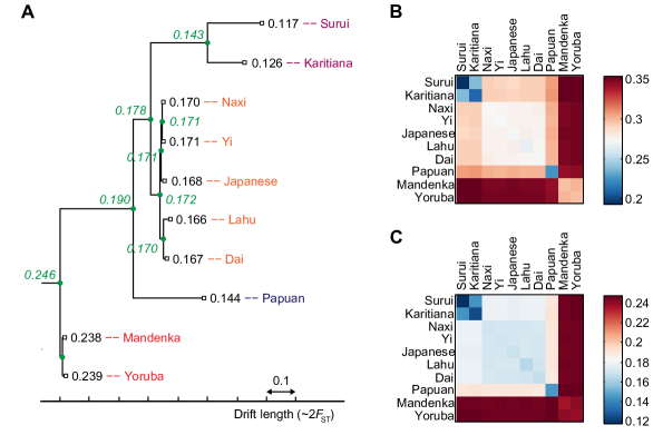
Figure 6: Ancestral heterozygosity imputed from original Illumina vs. San-ascertained SNPs. (A) The 10-population unadmixed tree with estimated average heterozygosities using SNPs from Panel 4 (San ascertainment) of the Affymetrix Human Origins array (?). Numbers in black are direct calculations for modern populations, while numbers in green are inferred values at ancestral nodes. (B, C) Computed ancestral heterozygosity at the common ancestor of each pair of modern populations. With unbiased data, values should be equal for pairs having the same common ancestor. (B) Values from a filtered subset of about 250,000 SNPs from the published Illumina array data (?). (C) Values from the Human Origins array excluding SNPs in gene regions.

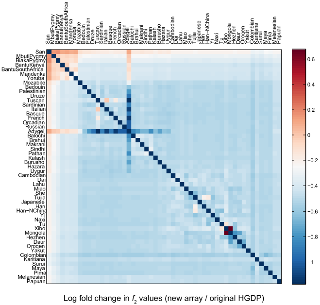
Figure S3: Comparison of $f_{2}$ distances computed using original Illumina vs. San-ascertained SNPs. The heat map shows the log fold change in $f_{2}$ values obtained from the original HGDP data (?) versus the San-ascertained data (?) used in this study.

Using SNPs ascertained in an outgroup to all of our study populations enables us to compute accurate estimates of the heterozygosity (over a given set of SNPs) throughout an unadmixed tree, including at ancestral nodes (see Material and Methods). This in turn allows us to convert branch lengths from $f_{2}$ units to easily interpretable drift lengths (see Text S2). In Figure 6C, we show our estimates for the heterozygosity (averaged over all San-ascertained SNPs used) at the most recent common ancestor (MRCA) of each pair of present-day populations in the tree. Consensus values are given at the nodes of Figure 6A. The imputed heterozygosity should be the same for each pair of populations with the same MRCA, and indeed, with the new data set, the agreement is excellent (Figure 6C). By contrast, inferences of ancestral heterozygosity are much less accurate using HGDP data from the original Illumina SNP array (?) because of ascertainment bias (Figure 6B); $f_{2}$ statistics are also affected but to a lesser degree (Figure S3), as previously demonstrated (?). We used these heterozygosity estimates to express branch lengths of all of our trees in drift units (Text S2).

Discussion

Comparison with previous approaches

The MixMapper framework generalizes and automates several previous admixture inference tools based on allele frequency moment statistics, incorporating them as special cases. Methods such as the 3-population test for admixture and $f_{4}$ ratio estimation (??) have similar theoretical underpinnings, but MixMapper provides more extensive information by analyzing more populations simultaneously and automatically considering different tree topologies and sources of gene flow. For example, negative $f_{3}$ values—i.e., 3-population tests indicating admixture—can be expressed in terms of relationships among $f_{2}$ distances between populations in an admixture tree. In general, 3-population tests can be somewhat difficult to interpret because the surrogate ancestral populations may not in fact be closely related to the true participants in the admixture, e.g., in the “outgroup case” (??). The relations among the $f_{2}$ statistics incorporate this situation naturally, however, and solving the full system recovers the true branch points wherever they are. As another example, $f_{4}$ ratio estimation infers mixture proportions of a single admixture event from $f_{4}$ statistics involving the admixed population and four unadmixed populations situated in a particular topology (??). Whenever data for five such populations are available, the system of all $f_{2}$ equations that MixMapper solves to obtain the mixture fraction becomes equivalent to the $f_{4}$ ratio computation. More importantly, because MixMapper infers all of the topological relationships within an admixture tree automatically by optimizing the solution of the distance equations over all branches, we do not need to specify in advance where the admixture took place—which is not always obvious a priori. By using more than five populations, MixMapper also benefits from more data points to constrain the fit.

MixMapper also offers significant advantages over the qpgraph admixture tree fitting software (?). Most notably, qpgraph requires the user to specify the entire topology of the tree, including admixtures, in advance. This requires either prior knowledge of sources of gene flow relative to the reference populations or a potentially lengthy search to test alternative branch locations. MixMapper is also faster and provides the capabilities to convert branch lengths into drift units and to perform bootstrap replicates to measure uncertainty in parameter estimates. Furthermore, MixMapper is designed to have more flexible and intuitive input and output and better diagnostics for incorrectly specified models. While qpgraph does fill a niche of fitting very precise models for small sets of populations, it becomes quite cumbersome for more than about seven or eight, whereas MixMapper can be run with significantly larger trees without sacrificing efficiency, ease of use, or accuracy of inferences for populations of interest.

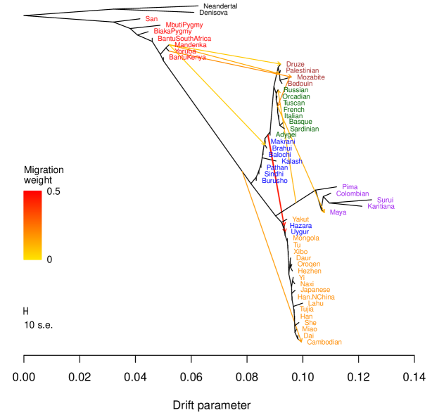
Figure S4: TreeMix results on the HGDP. Admixture graph for HGDP populations obtained with the TreeMix software, as reported in ?. Figure is reproduced from ? with permission of the authors and under the Creative Commons Attribution License.

Finally, MixMapper differs from TreeMix (?) in its emphasis on precise and flexible modeling of individual admixed populations. Stylistically, we view MixMapper as “semi-automated” as compared to TreeMix, which is almost fully automated. Both approaches have benefits: ours allows more manual guidance and lends itself to interactive use, whereas TreeMix requires less user intervention, although some care must be taken in choosing the number of gene flow events to include (10 in the HGDP results shown in Figure S4) to avoid creating spurious mixtures. With MixMapper, we create admixture trees including pre-selected approximately unadmixed populations together with admixed populations of interest, which are added on a case-by-case basis only if they fit reliably as two- or three-way admixtures. In contrast, TreeMix returns a single large-scale admixture tree containing all populations in the input data set, which may include some that can be shown to be admixed by other means but are not modeled as such. Thus, these populations might not be placed well on the tree, which in turn could affect the accuracy of the inferred admixture events. Likewise, the populations ultimately modeled as admixed are initially included as part of an unadmixed tree, where (presumably) they do not fit well, which could introduce errors in the starting tree topology that impact the final results.

Indeed, these methodological differences can be seen to affect inferences for both simulated and real data. For our second simulated admixture tree, MixMapper very accurately fit the populations with complicated histories (meant to mimic European and Middle Eastern populations), whereas TreeMix only recovered portions of the true tree and also added two inaccurate mixtures (Figure 3). We believe TreeMix was hindered in this case by attempting to fit all of the populations simultaneously and by starting with all of them in an unadmixed tree. In particular, once pop9 (with the lowest proportion of pop7-related admixture) was placed on the unadmixed tree, it likely became difficult to detect as admixed, while pop8’s initial placement higher up the tree was likely due to its pop2-related admixture but then obscured this signal in the mixture-fitting phase. Finally, the initial tree shape made populations 3-10 appear to be unequally drifted. Meanwhile, with the HGDP data (Figures 4 and S4), both methods fit Palestinian, Bedouin, Druze, Mozabite, Uygur, and Hazara as admixed, but MixMapper analysis suggested that these populations are better modeled as three-way admixed. TreeMix alone fit Brahui, Makrani, Cambodian, and Maya—all of which the 3-population test identifies as admixed but we were unable to place reliably with MixMapper—while MixMapper alone confidently fit Daur, Hezhen, Oroqen, Yakut, Melanesian, and Han. Perhaps most notably, MixMapper alone inferred widespread ancient admixture for Europeans; the closest possible signal of such an event in the TreeMix model is a migration edge from an ancestor of Native Americans to Russians. We believe that, as in the simulations, MixMapper is better suited to finding a common, ancient admixture signal in a group of populations, and more generally to disentangling complex admixture signals from within a large set of populations, and hence it is able to detect admixture in Europeans when TreeMix does not.

To summarize, MixMapper offers a suite of features that make it better suited than existing methods for the purpose of inferring accurate admixture parameters in data sets containing many specific populations of interest. Our approach provides a middle ground between qpgraph, which is designed to fit small numbers of populations within almost no residual errors, and TreeMix, which generates large trees with little manual intervention but may be less precise in complex admixture scenarios. Moreover, MixMapper’s speed and interactive design allow the user to evaluate the uncertainty and robustness of results in ways that we have found to be very useful (e.g., by comparing two- vs. three-way admixture models or results obtained using alternative scaffold trees).

Ancient European admixture

Due in part to the flexibility of the MixMapper approach, we were able to obtain the notable result that all European populations in the HGDP are best modeled as mixtures between a population related to the common ancestor of Native Americans and a population related to the common ancestor of all non-African populations in our scaffold tree, confirming and extending an admixture signal first reported by ?. Our interpretation is that most if not all modern Europeans are descended from at least one large-scale ancient admixture event involving, in some combination, at least one population of Mesolithic European hunter-gatherers; Neolithic farmers, originally from the Near East; and/or other migrants from northern or Central Asia. Either the first or second of these could be related to the “ancient western Eurasian” branch in Figure 5, and either the first or third could be related to the “ancient northern Eurasian” branch. Present-day Europeans differ in the amount of drift they have experienced since the admixture and in the proportions of the ancestry components they have inherited, but their overall profiles are similar.

Our results for Europeans are consistent with several previously published lines of evidence (?). First, it has long been hypothesized, based on analysis of a few genetic loci (especially on the Y chromosome), that Europeans are descended from ancient admixtures (???). Our results also suggest an interpretation for a previously unexplained frappe analysis of worldwide human population structure (using $K=4$ clusters) showing that almost all Europeans contain a small fraction of American-related ancestry (?). Finally, sequencing of ancient DNA has revealed substantial differentiation in Neolithic Europe between farmers and hunter-gatherers (?), with the former more closely related to present-day Middle Easterners (?) and southern Europeans (??) and the latter more similar to northern Europeans (?), a pattern perhaps reflected in our observed northwest-southeast cline in the proportion of “ancient northern Eurasian” ancestry (Table 1). Further analysis of ancient DNA may help shed more light on the sources of ancestry of modern Europeans (?).

One important new insight of our European analysis is that we detect the same signal of admixture in Sardinian and Basque as in the rest of Europe. As discussed above, unlike other Europeans, Sardinian and Basque cannot be confirmed to be admixed using the 3-population test (as in ?), likely due to a combination of less “ancient northern Eurasian” ancestry and more genetic drift since the admixture (Table 1). The first point is further complicated by the fact that we have no unadmixed “ancient western Eurasian” population available to use as a reference; indeed, Sardinians themselves are often taken to be such a reference. However, MixMapper uncovered strong evidence for admixture in Sardinian and Basque through additivity-checking in the first phase of the program and automatic topology optimization in the second phase, discovering the correct arrangement of unadmixed populations and enabling admixture parameter inference, which we then verified directly with $f_{4}$ ratio estimation. Perhaps the most convincing evidence of the robustness of this finding is that MixMapper infers branch points for the ancestral mixing populations that are very similar to those of other Europeans (Table 1), a concordance that is most parsimoniously explained by a shared history of ancient admixture among Sardinian, Basque, and other European populations. Finally, we note that because we fit all European populations without assuming Sardinian or Basque to be an unadmixed reference, our estimates of the “ancient northern Eurasian” ancestry proportions in Europeans are larger than those in ? and we believe more accurate than others previously reported (?).

Future directions

It is worth noting that of the 52 populations (excluding San) in the HGDP data set, there were 22 that we were unable to fit in a reasonable way either on the unadmixed tree or as admixtures. In part, this was because our instantaneous-admixture model is intrinsically limited in its ability to capture complicated population histories. Most areas of the world have surely witnessed ongoing low levels of inter-population migration over time, especially between nearby populations, making it difficult to fit admixture trees to the data. We also found cases where having data from more populations would help the fitting process, for example for three-way admixed populations such as Maya where we do not have a sampled group with a simpler admixture history that could be used to represent two of the three components. Similarly, we found that while Central Asian populations such as Burusho, Pathan, and Sindhi have clear signals of admixture from the 3-population test, their ancestry can likely be traced to several different sources (including sub-Saharan Africa in some instances), making them difficult to fit with MixMapper, particularly using the HGDP data. Finally, we have chosen here to disregard admixture with archaic humans, which is known to be a small but noticeable component for most populations in the HGDP (??). In the future, it will be interesting to extend MixMapper and other admixture tree-fitting methods to incorporate the possibilities of multiple-wave and continuous admixture.

In certain applications, full genome sequences are beginning to replace more limited genotype data sets such as ours, but we believe that our methods and SNP-based inference in general will still be valuable in the future. Despite the improving cost-effectiveness of sequencing, it is still much easier and less expensive to genotype samples using a SNP array, and with over 100,000 loci, the data used in this study provide substantial statistical power. Additionally, sequencing technology is currently more error-prone, which can lead to biases in allele frequency-based statistics (?).We expect that MixMapper will continue to contribute to an important toolkit of population history inference methods based on SNP allele frequency data.

Material and Methods

Model assumptions and $f$-statistics

We assume that all SNPs are neutral, biallelic, and autosomal, and that divergence times are short enough that there are no double mutations at a locus. Thus, allele frequency variation—the signal that we harness—is governed entirely by genetic drift and admixture. We model admixture as a one-time exchange of genetic material: two parent populations mix to form a single descendant population whose allele frequencies are a weighted average of the parents’. This model is of course an oversimplification of true mixture events, but it is flexible enough to serve as a first-order approximation.

Our point-admixture model is amenable to allele frequency moment analyses based on $f$-statistics (??). We primarily make use of the statistic $f_{2}(A,B):=E_{S}[(p_{A}-p_{B})^{2}]$, where $p_{A}$ and $p_{B}$ are allele frequencies in populations $A$ and $B$, and $E_{S}$ denotes the mean over all SNPs. Expected values of $f_{2}$ can be written in terms of admixture tree parameters as described in Text S1. Linear combinations of $f_{2}$ statistics can also be used to form the quantities $f_{3}(C;A,B):=E_{S}[(p_{C}-p_{A})(p_{C}-p_{B})]$ and $f_{4}(A,B;C,D):=E_{S}[(p_{A}-p_{B})(p_{C}-p_{D})]$, which form the bases of the 3- and 4-population tests for admixture, respectively. For all of our $f$-statistic computations, we use previously described unbiased estimators (??).

Constructing an unadmixed scaffold tree

Our MixMapper admixture-tree-building procedure consists of two phases (Figure 1), the first of which selects a set of unadmixed populations to use as a scaffold tree. We begin by computing $f_{3}$ statistics (??) for all triples of populations $P_{1},P_{2},P_{3}$ in the data set and removing those populations $P_{3}$ with any negative values $f_{3}(P_{3};P_{1},P_{2})$, which indicate admixture. We then use pairwise $f_{2}$ statistics to build neighbor-joining trees on subsets of the remaining populations. In the absence of admixture, $f_{2}$ distances are additive along paths on a phylogenetic tree (Text S1; cf. ?), meaning that neighbor-joining should recover a tree with leaf-to-leaf distances that are completely consistent with the pairwise $f_{2}$ data (?). However, with real data, the putative unadmixed subsets are rarely completely additive, meaning that the fitted neighbor-joining trees have residual errors between the inferred leaf-to-leaf distances and the true $f_{2}$ statistics. These deviations from additivity are equivalent to non-zero results from the 4-population test for admixture (??). We therefore evaluate the quality of each putative unadmixed tree according to its maximum error between fitted and actual pairwise distances: for a tree $\mathit{T}$ having distances $d$ between populations $P$ and $Q$, the deviation from additivity is defined as $\max\{|d(P,Q)-f_{2}(P,Q)|:P,Q\in\mathit{T}\}$. MixMapper computes this deviation on putatively unadmixed subsets of increasing size, retaining a user-specified number of best subsets of each size in a “beam search” procedure to avoid exponential complexity.

Because of model violations in real data, trees built on smaller subsets are more additive, but they are also less informative; in particular, it is beneficial to include populations from as many continental groups as possible in order to provide more potential branch points for admixture fitting. MixMapper provides a ranking of the most additive trees of each size as a guide from which the user chooses a suitable unadmixed scaffold. Once the rank-list of trees has been generated, subject to some constraints (e.g., certain populations required), the user can scan the first several most additive trees for a range of sizes, looking for a balance between coverage and accuracy. This can also be accomplished by checking whether removing a population from a proposed tree results in a substantial additivity benefit; if so, it may be wise to eliminate it. Similarly, if the population removed from the tree can be modeled well as admixed using the remaining portion of the scaffold, this provides evidence that it should not be part of the unadmixed tree. Finally, MixMapper adjusts the scaffold tree that the user ultimately selects by re-optimizing its branch lengths (maintaining the topology inferred from neighbor-joining) to minimize the sum of squared errors of all pairwise $f_{2}$ distances.

Within the above guidelines, users should choose the scaffold tree most appropriate for their purposes, which may involve other considerations. In addition to additivity and overall size, it is sometimes desirable to select more or fewer populations from certain geographical, linguistic, or other categories. For example, including a population in the scaffold that is actually admixed might not affect the inferences as long as it is not too closely related to the admixed populations being modeled. At the same time, it can be useful to have more populations in the scaffold around the split points for an admixed population of interest in order to obtain finer resolution on the branch positions of the mixing populations. For human data in particular, the unadmixed scaffold is only a modeling device; the populations it contains likely have experienced at least a small amount of mixture. A central goal in building the scaffold is to choose populations such that applying this model will not interfere with the conclusions obtained using the program. The interactive design of MixMapper allows the user to tweak the scaffold tree very easily in order to check robustness, and in our analyses, conclusions are qualitatively unchanged for different scaffolds (Figures S1–S2; Tables S2–S4).

Two-way admixture fitting

The second phase of MixMapper begins by attempting to fit additional populations independently as simple two-way admixtures between branches of the unadmixed tree (Figure 1). For a given admixed population, assuming for the moment that we know the branches from which the ancestral mixing populations split, we can construct a system of equations of $f_{2}$ statistics that allows us to infer parameters of the mixture (Text S1). Specifically, the squared allele frequency divergence $f_{2}(M,X^{\prime})$ between the admixed population $M$ and each unadmixed population $X^{\prime}$ can be expressed as an algebraic combination of known branch lengths along with four unknown mixture parameters: the locations of the split points on the two parental branches, the combined terminal branch length, and the mixture fraction (Figure 2A). To solve for the four unknowns, we need at least four unadmixed populations $X^{\prime}$ that produce a system of four independent constraints on the parameters. This condition is satisfied if and only if the data set contains two populations $X^{\prime}_{1}$ and $X^{\prime}_{2}$ that branch from different points along the lineage connecting the divergence points of the parent populations from the unadmixed tree (Text S1). If the unadmixed tree contains $n>4$ populations, we obtain a system of $n$ equations in the four unknowns that in theory is dependent. In practice, the equations are in fact slightly inconsistent because of noise in the $f_{2}$ statistics and error in the point-admixture model, so we perform least-squares optimization to solve for the unknowns; having more populations helps reduce the impact of noise.

Algorithmically, MixMapper performs two-way admixture fitting by iteratively testing each pair of branches of the unadmixed tree as possible sources of the two ancestral mixing populations. For each choice of branches, MixMapper builds the implied system of equations and finds the least-squares solution (under the constraints that unknown branch lengths are nonnegative and the mixture fraction $\alpha$ is between 0 and 1), ultimately choosing the pair of branches and mixture parameters producing the smallest residual norm. Our procedure for optimizing each system of equations uses the observation that upon fixing $\alpha$, the system becomes linear in the remaining three variables (Text S1). Thus, we can optimize the system by performing constrained linear least squares within a basic one-parameter optimization routine over $\alpha\in[0,1]$. To implement this approach, we applied MATLAB’s lsqlin and fminbnd functions with a few auxiliary tricks to improve computational efficiency (detailed in the code).

Three-way admixture fitting

MixMapper also fits three-way admixtures, i.e., those for which one parent population is itself admixed (Figure 2B). Explicitly, after an admixed population $M_{1}$ has been added to the tree, MixMapper can fit an additional user-specified admixed population $M_{2}$ as a mixture between the $M_{1}$ terminal branch and another (unknown) branch of the unadmixed tree. The fitting algorithm proceeds in a manner analogous to the two-way mixture case: MixMapper iterates through each possible choice of the third branch, optimizing each implied system of equations expressing $f_{2}$ distances in terms of mixture parameters. With two admixed populations, there are now $2n+1$ equations, relating observed values of $f_{2}(M_{1},X^{\prime})$ and $f_{2}(M_{2},X^{\prime})$ for all unadmixed populations $X^{\prime}$, and also $f_{2}(M_{1},M_{2})$, to eight unknowns: two mixture fractions, $\alpha_{1}$ and $\alpha_{2}$, and six branch length parameters (Figure 2B). Fixing $\alpha_{1}$ and $\alpha_{2}$ results in a linear system as before, so we perform the optimization using MATLAB’s lsqlin within fminsearch applied to $\alpha_{1}$ and $\alpha_{2}$ in tandem. The same mathematical framework could be extended to optimizing the placement of populations with arbitrarily many ancestral admixture events, but for simplicity and to reduce the risk of overfitting, we chose to limit this version of MixMapper to three-way admixtures.

Expressing branch lengths in drift units

All of the tree-fitting computations described thus far are performed using pairwise distances in $f_{2}$ units, which are mathematically convenient to work with owing to their additivity along a lineage (in the absence of admixture). However, $f_{2}$ distances are not directly interpretable in the same way as genetic drift $D$, which is a simple function of time and population size:

$$D\approx 1-\exp(-t/2N_{e})\approx 2\cdot F_{ST},$$

where $t$ is the number of generations and $N_{e}$ is the effective population size (?). To convert $f_{2}$ distances to drift units, we apply a new formula, dividing twice the $f_{2}$-length of each branch by the heterozygosity value that we infer for the ancestral population at the top of the branch (Text S2). Qualitatively speaking, this conversion corrects for the relative stretching of $f_{2}$ branches at different portions of the tree as a function of heterozygosity (?). In order to infer ancestral heterozygosity values accurately, it is critical to use SNPs that are ascertained in an outgroup to the populations involved, which we address further below.

Before inferring heterozygosities at ancestral nodes of the unadmixed tree, we must first determine the location of the root (which is neither specified by neighbor-joining nor involved in the preceding analyses). MixMapper does so by iterating through branches of the unadmixed tree, temporarily rooting the tree along each branch, and then checking for consistency of the resulting heterozygosity estimates. Explicitly, for each internal node $P$, we split its present-day descendants (according to the re-rooted tree) into two groups $G_{1}$ and $G_{2}$ according to which child branch of $P$ they descend from. For each pair of descendants, one from $G_{1}$ and one from $G_{2}$, we compute an inferred heterozygosity at $P$ (Text S2). If the tree is rooted properly, these inferred heterozygosities are consistent, but if not, there exist nodes $P$ for which the heterozygosity estimates conflict. MixMapper thus infers the location of the root as well as the ancestral heterozygosity at each internal node, after which it applies the drift length conversion as a post-processing step on fitted $f_{2}$ branch lengths.

Bootstrapping

In order to measure the statistical significance of our parameter estimates, we compute bootstrap confidence intervals (??) for the inferred branch lengths and mixture fractions. Our bootstrap procedure is designed to account for both the randomness of the drift process at each SNP and the random choice of individuals sampled to represent each population. First, we divide the genome into 50 evenly-sized blocks, with the premise that this scale should easily be larger than that of linkage disequilibrium among our SNPs. Then, for each of 500 replicates, we resample the data set by (a) selecting 50 of these SNP blocks at random with replacement; and (b) for each population group, selecting a random set of individuals with replacement, preserving the number of individuals in the group.

For each replicate, we recalculate all pairwise $f_{2}$ distances and present-day heterozygosity values using the resampled SNPs and individuals (adjusting the bias-correction terms to account for the repetition of individuals) and then construct the admixture tree of interest. Even though the mixture parameters we estimate—branch lengths and mixture fractions—depend in complicated ways on many different random variables, we can directly apply the nonparametric bootstrap to obtain confidence intervals (?). For simplicity, we use a percentile bootstrap; thus, our 95% confidence intervals indicate 2.5 and 97.5 percentiles of the distribution of each parameter among the replicates.

Computationally, we parallelize MixMapper’s mixture-fitting over the bootstrap replicates using MATLAB’s Parallel Computing Toolbox.

Evaluating fit quality

When interpreting admixture inferences produced by methods such as MixMapper, it is important to ensure that best-fit models are in fact accurate. While formal tests for goodness of fit do not generally exist for methods of this class, we use several criteria to evaluate the mixture fits produced by MixMapper and distinguish high-confidence results from possible artifacts of overfitting or model violations.

First, we can compare MixMapper results to information obtained from other methods, such as the 3-population test (??). Negative $f_{3}$ values indicate robustly that the tested population is admixed, and comparing $f_{3}$ statistics for different reference pairs can give useful clues about the ancestral mixing populations. Thus, while the 3-population test relies on similar data to MixMapper, its simpler form makes it useful for confirming that MixMapper results are reasonable.

Second, the consistency of parameter values over bootstrap replicates gives an indication of the robustness of the admixture fit in question. All results with real data have some amount of associated uncertainty, which is a function of sample sizes, SNP density, intra-population homogeneity, and other aspects of the data. Given these factors, we place less faith in results with unexpectedly large error bars. Most often, this phenomenon is manifested in the placement of ancestral mixing populations: for poorly fitting admixtures, branch choices often change from one replicate to the next, signaling unreliable results.

Third, we find that results where one ancestral population is very closely related to the admixed population and contributes more than 90% of the ancestry are often unreliable. We expect that if we try to fit a non-admixed population as an admixture, MixMapper should return a closely related population as the first branch with mixture fraction $\alpha\approx 1$ (and an arbitrary second branch). Indeed, we often observe this pattern in the context of verifying that certain populations make sense to include in the scaffold tree. Further evidence of overfitting comes when the second ancestry component, which contributes only a few percent, either bounces from branch to branch over the replicates, is located at the very tip of a leaf branch, or is historically implausible.

Fourth, for any inferred admixture event, the two mixing populations must be contemporaneous. Since we cannot resolve the three pieces of terminal drift lengths leading to admixed populations (Figure 2A) and our branch lengths depend both on population size and absolute time, we cannot say for sure whether this property is satisfied for any given mixture fit. In some cases, however, it is clear that no realization of the variables could possibly be consistent: for example, if we infer an admixture between a very recent branch and a very old one with a small value of the total mixed drift—and hence the terminal drift $c$—then we can confidently say the mixture is unreasonable.

Finally, when available, we also use prior historical or other external knowledge to guide what we consider to be reasonable. Sometimes, the model that appears to fit the data best has implications that are clearly historically implausible; often when this is true one or more of the evaluation criteria listed above can be invoked as well. Of course, the most interesting findings are often those that are new and surprising, but we subject such results to an extra degree of scrutiny.

Data set and ascertainment

We analyzed a SNP data set from 934 HGDP individuals grouped in 53 populations (??). Unlike most previous studies of the HGDP samples, however, we worked with recently published data generated using the new Affymetrix Axiom Human Origins Array (?), which was designed with a simple ascertainment scheme for accurate population genetic inference (?). It is well known that ascertainment bias can cause errors in estimated divergences among populations (??), since choosing SNPs based on their properties in modern populations induces non-neutral spectra in related samples. While there do exist methods to correct for ascertainment bias (?), it is much more desirable to work with a priori bias-free data, especially given that typical SNP arrays are designed using opaque ascertainment schemes.

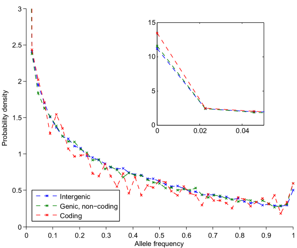
Figure S5: Comparison of allele frequency spectra within and outside gene regions. We divided the Panel 4 (San-ascertained) SNPs into three groups: those outside gene regions (101,944), those within gene regions but not in exons (58,110), and those within coding regions (3259). Allele frequency spectra restricted to each group are shown for the Yoruba population. Reduced heterozygosity within exon regions is evident, which suggests the action of purifying selection. (Inset) We observe the same effect in the genic, non-coding spectrum; it is less noticeable but can be seen at the edge of the spectrum.

To avoid these pitfalls, we used Panel 4 of the new array, which consists of 163,313 SNPs that were ascertained as heterozygous in the genome of a San individual (?). This panel is special because there is evidence that the San are approximately an outgroup to all other modern-day human populations (??). Thus, while the Panel 4 ascertainment scheme distorts the San allele frequency spectrum, it is nearly neutral with respect to all other populations. In other words, we can think of the ascertainment as effectively choosing a set of SNPs (biased toward San heterozygosity) at the common ancestor of the remaining 52 populations, after which drift occurs in a bias-free manner. We excluded 61,369 SNPs that are annotated as falling between the transcription start site and end site of a gene in the UCSC Genome Browser database (?). Most of the excluded SNPs are not within actual exons, but as expected, the frequency spectra at these “gene region” loci were slightly shifted toward fixed classes relative to other SNPs, indicative of the action of selection (Figure S5). Since we assume neutrality in all of our analyses, we chose to remove these SNPs.

Simulations

Our first simulated tree was generated using the ms (?) command

ms 350 500 -t 50 -r 99.9998 500000 -I 7 50 50 50 50 50 50 50 -n 7 2 -n 1 2 -n 2 2 -ej 0.04 2 1 -es 0.02 6 0.4 -ej 0.06 6 3 -ej 0.04 8 5 -ej 0.08 5 4 -ej 0.12 4 3 -ej 0.2 3 1 -ej 0.3 1 7 -en 0.3 7 1.

After ascertainment, we used a total of 95,997 SNPs.

Our second simulated tree was generated with the command

ms 550 500 -t 50 -r 99.9998 500000 -I 11 50 50 50 50 50 50 50 50 50 50 50 -n 11 2 -n 1 2 -n 2 2 -em 0.002 4 3 253.8 -em 0.004 4 3 0 -es 0.002 8 0.2 -en 0.002 8 2 -ej 0.02 8 2 -ej 0.02 4 5 -ej 0.04 2 1 -ej 0.04 5 3 -es 0.04 12 0.4 -es 0.04 9 0.2 -em 0.042 10 9 253.8 -em 0.044 10 9 0 -ej 0.06 12 7 -ej 0.06 9 7 -ej 0.06 14 10 -ej 0.06 13 10 -ej 0.08 7 6 -ej 0.12 6 3 -ej 0.16 10 3 -ej 0.2 3 1 -ej 0.3 1 11 -en 0.3 11 1.

After ascertainment, we used a total of 96,258 SNPs. When analyzing this data set in TreeMix, we chose to fit a total of five admixtures based on the residuals of the pairwise distances (maximum of approximately 3 standard errors) and our knowledge that this is the number in the true admixture tree (in order to make for a fair comparison).

Software

Source code for the MixMapper software is available at http://groups.csail.mit.edu/cb/mixmapper/.

Figures

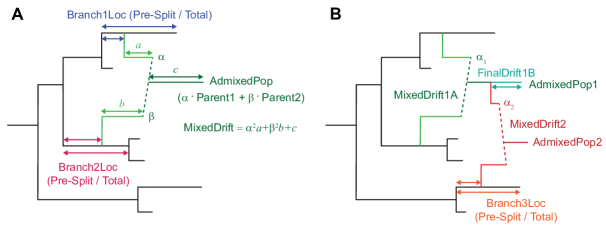
Figure 2: Schematic of mixture parameters fit by MixMapper. (A) A simple two-way admixture. MixMapper infers four parameters when fitting a given population as an admixture. It finds the optimal pair of branches between which to place the admixture and reports the following: Branch1Loc and Branch2Loc are the points at which the mixing populations split from these branches (given as pre-split length / total branch length); $\alpha$ is the proportion of ancestry from Branch1 ($\beta=1-\alpha$ is the proportion from Branch2); and MixedDrift is the linear combination of drift lengths $\alpha^{2}a+\beta^{2}b+c$. (B) A three-way mixture: here AdmixedPop2 is modeled as an admixture between AdmixedPop1 and Branch3. There are now four additional parameters; three are analogous to the above, namely, Branch3Loc, $\alpha_{2}$, and MixedDrift2. The remaining degree of freedom is the position of the split along the AdmixedPop1 branch, which divides MixedDrift into MixedDrift1A and FinalDrift1B.

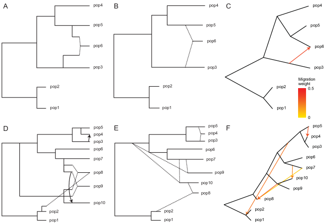
Figure 3: Results with simulated data. (A-C) First simulated admixture tree, with one admixed population. Shown are: (A) the true phylogeny, (B) MixMapper results, and (C) TreeMix results. (D-F) Second simulated admixture tree, with four admixed populations. Shown are: (D) the true phylogeny, (E) MixMapper results, and (F) TreeMix results. In (A) and (D), dotted lines indicate instantaneous admixtures, while arrows denote continuous (unidirectional) gene flow over 40 generations. Both MixMapper and TreeMix infer point admixtures, depicted with dotted lines in (B) and (E) and colored arrows in (C) and (F). In (B) and (E), the terminal drift edges shown for admixed populations represent half the total mixed drift. Full inferred parameters from MixMapper are given in Table S1.

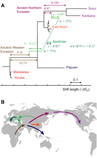
Figure 5: Inferred ancient admixture in Europe. (A) Detail of the inferred ancestral admixture for Sardinians (other European populations are similar). One mixing population splits from the unadmixed tree along the common ancestral branch of Native Americans (“Ancient Northern Eurasian”) and the other along the common ancestral branch of all non-Africans (“Ancient Western Eurasian”). Median parameter values are shown; 95% bootstrap confidence intervals can be found in Table 1. The branch lengths $a$, $b$, and $c$ are confounded, so we show a plausible combination. (B) Map showing a sketch of possible directions of movement of ancestral populations. Colored arrows correspond to labeled branches in (A).

Tables

Table 1: Mixture parameters for Europeans.

AdmixedPop	# repa	$\alpha$b	Branch1Loc (Anc. N. Eurasian)c	Branch2Loc (Anc. W. Eurasian)c	MixedDriftd
Adygei	500	0.254-0.461	0.033-0.078 / 0.195	0.140-0.174 / 0.231	0.077-0.092
Basque	464	0.160-0.385	0.053-0.143 / 0.196	0.149-0.180 / 0.231	0.105-0.121
French	491	0.184-0.386	0.054-0.130 / 0.195	0.149-0.177 / 0.231	0.089-0.104
Italian	497	0.210-0.415	0.043-0.108 / 0.195	0.137-0.173 / 0.231	0.092-0.109
Orcadian	442	0.156-0.350	0.068-0.164 / 0.195	0.161-0.185 / 0.231	0.096-0.113
Russian	500	0.278-0.486	0.045-0.091 / 0.195	0.146-0.181 / 0.231	0.079-0.095
Sardinian	480	0.150-0.350	0.045-0.121 / 0.195	0.146-0.176 / 0.231	0.107-0.123
Tuscan	489	0.179-0.431	0.039-0.118 / 0.195	0.137-0.177 / 0.231	0.088-0.110

^aNumber of bootstrap replicates (out of 500) placing the mixture between the two branches shown.

^bProportion of ancestry from “ancient northern Eurasian” (95% bootstrap confidence interval).

^cSee Figure 5A for the definition of the “ancient northern Eurasian” and “ancient western Eurasian” branches in the scaffold tree; Branch1Loc and Branch2Loc are the points at which the mixing populations split from these branches (expressed as confidence interval for split point / branch total, as in Figure 2A).

^dSum of drift lengths $\alpha^{2}a+(1-\alpha)^{2}b+c$; see Figure 2A.

Table 2: Mixture parameters for non-European populations modeled as two-way admixtures.

AdmixedPop	Branch1 + Branch2a	# repb	$\alpha$c	Branch1Locd	Branch2Locd	MixedDrifte
Daur	Anc. N. Eurasian + Japanese	350	0.067-0.276	0.008-0.126 / 0.195	0.006-0.013 / 0.016	0.006-0.015
	Suruí + Japanese	112	0.021-0.058	0.008-0.177 / 0.177	0.005-0.010 / 0.015	0.005-0.016
Hezhen	Anc. N. Eurasian + Japanese	411	0.068-0.273	0.006-0.113 / 0.195	0.006-0.013 / 0.016	0.005-0.029
Oroqen	Anc. N. Eurasian + Japanese	410	0.093-0.333	0.017-0.133 / 0.195	0.005-0.013 / 0.015	0.011-0.030
	Karitiana + Japanese	53	0.025-0.086	0.014-0.136 / 0.136	0.004-0.008 / 0.016	0.008-0.026
Yakut	Anc. N. Eurasian + Japanese	481	0.494-0.769	0.005-0.026 / 0.195	0.012-0.016 / 0.016	0.030-0.041
Melanesian	Dai + Papuan	424	0.160-0.260	0.008-0.014 / 0.014	0.165-0.201 / 0.247	0.089-0.114
	Lahu + Papuan	54	0.155-0.255	0.003-0.032 / 0.032	0.167-0.208 / 0.249	0.081-0.114
Han	Dai + Japanese	440	0.349-0.690	0.004-0.014 / 0.014	0.008-0.016 / 0.016	0.002-0.006

^aOptimal split points for mixing populations.

^bNumber of bootstrap replicates (out of 500) placing the mixture between Branch1 and Branch2; topologies are shown that that occur for at least 50 of 500 replicates.

^cProportion of ancestry from Branch1 (95% bootstrap confidence interval).

^dPoints at which mixing populations split from their branches (expressed as confidence interval for split point / branch total, as in Figure 2A).

^eSum of drift lengths $\alpha^{2}a+(1-\alpha)^{2}b+c$; see Figure 2A.

Table 3: Mixture parameters for populations modeled as three-way admixtures.

AdmixedPop2	Branch3a	# repb	$\alpha_{2}$c	Branch3Locd	MixedDrift1Ae	FinalDrift1Be	MixedDrift2e
Druze	Mandenka	330	0.963-0.988	0.000-0.009 / 0.009	0.081-0.099	0.022-0.030	0.004-0.013
	Yoruba	82	0.965-0.991	0.000-0.010 / 0.010	0.080-0.099	0.022-0.029	0.005-0.013
	Anc. W. Eurasian	79	0.881-0.966	0.041-0.158 / 0.232	0.092-0.118	0.000-0.024	0.010-0.031
Palestinian	Anc. W. Eurasian	294	0.818-0.901	0.031-0.104 / 0.231	0.093-0.123	0.000-0.021	0.007-0.022
	Mandenka	146	0.909-0.937	0.000-0.009 / 0.009	0.083-0.097	0.022-0.029	0.001-0.007
	Yoruba	53	0.911-0.938	0.000-0.010 / 0.010	0.077-0.098	0.021-0.029	0.001-0.008
Bedouin	Anc. W. Eurasian	271	0.767-0.873	0.019-0.086 / 0.231	0.094-0.122	0.000-0.022	0.012-0.031
	Mandenka	176	0.856-0.923	0.000-0.008 / 0.008	0.080-0.099	0.023-0.030	0.006-0.018
Mozabite	Mandenka	254	0.686-0.775	0.000-0.009 / 0.009	0.088-0.109	0.012-0.022	0.017-0.032
	Anc. W. Eurasian	142	0.608-0.722	0.002-0.026 / 0.232	0.103-0.122	0.000-0.011	0.018-0.035
	Yoruba	73	0.669-0.767	0.000-0.008 / 0.010	0.086-0.108	0.012-0.023	0.017-0.031
Hazara	Anc. East Asianf	497	0.364-0.471	0.010-0.024 / 0.034	0.080-0.115	0.004-0.034	0.004-0.013
Uygur	Anc. East Asianf	500	0.318-0.438	0.007-0.023 / 0.034	0.088-0.123	0.000-0.027	0.000-0.009

^aOptimal split point for the third ancestry component. The first two components are represented by a parent population splitting from the (admixed) Sardinian branch.

^bNumber of bootstrap replicates placing the third ancestry component on Branch3; topologies are shown that that occur for at least 50 of 500 replicates.

^cProportion of European-related ancestry (95% bootstrap confidence interval).

^dPoint at which mixing population splits from Branch3 (expressed as confidence interval for split point / branch total, as in Figure 2A).

^eTerminal drift parameters; see Figure 2B.

^fCommon ancestral branch of the five East Asian populations in the unadmixed tree (Dai, Japanese, Lahu, Naxi, and Yi).

Supplementary Materials: Efficient moment-based inference of admixture parameters and sources of gene flow

Mark Lipson, Po-Ru Loh, Alex Levin, David Reich, Nick Patterson, and Bonnie Berger

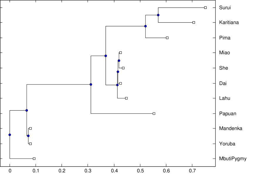
Figure S1: Alternative scaffold tree with 11 populations used to evaluate robustness of results to scaffold choice. We included Mbuti Pygmy, who are known to be admixed, to help demonstrate that MixMapper inferences are robust to deviations from additivity in the scaffold; see Tables S2–S4 for full results. Distances are in drift units.

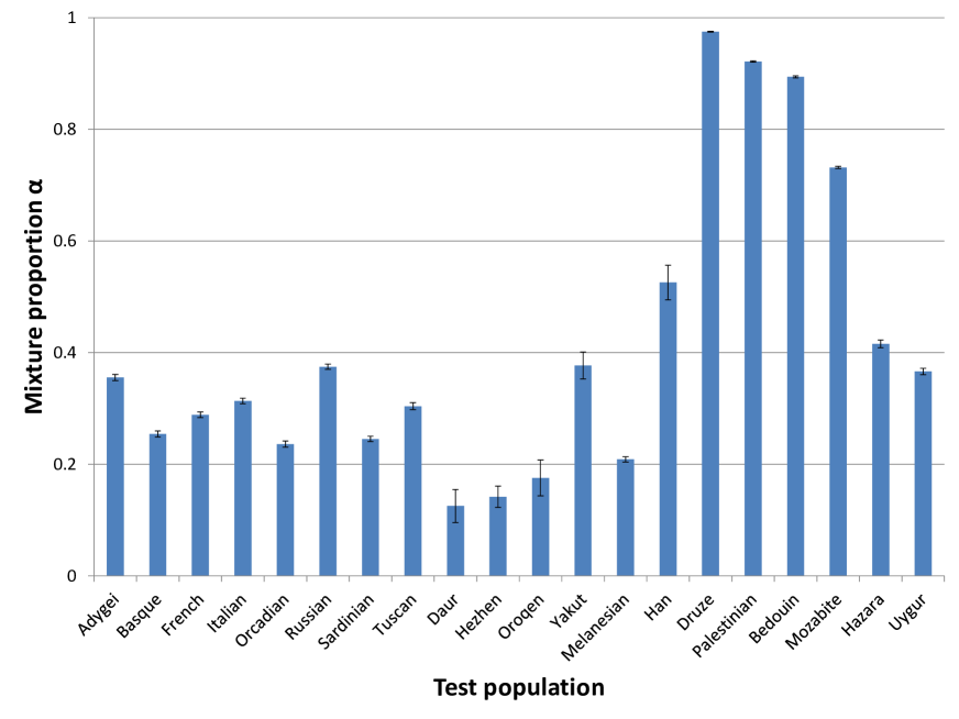
Figure S2: Summary of mixture proportions $\alpha$ inferred with alternative 9-population scaffold trees. We ran MixMapper for all 20 admixed test populations using nine different scaffold trees obtained by removing each population except Papuan one at a time from our full 10-population scaffold. (Papuan is needed to maintain continental representation.) For each test population and each scaffold, we recorded the median bootstrap-inferred value of $\alpha$ over all replicates having branching patterns similar to the primary topology. Shown here are the means and standard deviations of the nine medians. In all cases, $\alpha$ refers to the proportion of ancestry from the first branch as in Tables 1–3.

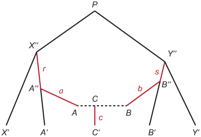
Figure S6: Schematic of part of an admixture tree. Population $C$ is derived from an admixture of populations $A$ and $B$ with proportion $\alpha$ coming from $A$. The $f_{2}$ distances from $C^{\prime}$ to the present-day populations $A^{\prime},B^{\prime},X^{\prime},Y^{\prime}$ give four relations from which we are able to infer four parameters: the mixture fraction $\alpha$, the locations of the split points $A^{\prime\prime}$ and $B^{\prime\prime}$ (i.e., $r$ and $s$), and the combined drift $\alpha^{2}a+(1-\alpha)^{2}b+c$.

Table S1: Mixture parameters for simulated data.

AdmixedPop	Branch1 + Branch2	# rep	$\alpha$	Branch1Loc	Branch2Loc	MixedDrift
First tree
pop6	pop3 + pop5	500	0.253-0.480	0.078-0.195 / 0.214	0.050-0.086 / 0.143	0.056-0.068
pop6 (true)	pop3 + pop5		0.4	0.107 / 0.213	0.077 / 0.145	0.066
Second tree
pop4	pop3 + pop5	500	0.382-0.652	0.039-0.071 / 0.076	0.032-0.073 / 0.077	0.010-0.020
pop4 (true)	pop3 + pop5		0.4	0.071 / 0.077	0.038 / 0.077	0.016
pop9	Anc3–7 + pop7	490	0.653-0.915	0.048-0.091 / 0.140	0.013-0.134 / 0.147	0.194-0.216
pop9 (true)	Anc3–7 + pop7		0.8	0.077 / 0.145	0.037 / 0.145	0.194
pop10	Anc3–7 + pop7	500	0.502-0.690	0.047-0.091 / 0.140	0.021-0.067 / 0.147	0.151-0.167
pop10 (true)	Anc3–7 + pop7		0.6	0.077 / 0.145	0.037 / 0.145	0.150
AdmixedPop2	AdmixedPop1 + Branch3	# rep	$\alpha_{2}$	Branch3Loc
pop8	pop10 + pop2	304	0.782-0.822	0.007-0.040 / 0.040
	pop10 + Anc1–2	193	0.578-0.756	0.009-0.104 / 0.148
pop8 (true)	pop10 + pop2		0.8	0.020 / 0.039

Note.—Mixture parameters inferred by MixMapper for simulated data, followed by true values for each simulated admixed population. Branch1 and Branch2 are the optimal split points for the mixing populations, with $\alpha$ the proportion of ancestry from Branch1; topologies are shown that that occur for at least 20 of 500 bootstrap replicates. The mixed drift parameters for the three-way admixed pop8 are not well-defined in the simulated tree and are omitted. The branch “Anc3–7” is the common ancestral branch of pops 3–7, and the branch “Anc1–2” is the common ancestral branch of pops 1–2. See Figure 2 and the caption of Table 1 for descriptions of the parameters and Figure 3 for plots of the results.

Table S2: Mixture parameters for Europeans inferred with an alternative scaffold tree.

AdmixedPop	# rep	$\alpha$	Branch1Loc (Anc. N. Eurasian)	Branch2Loc (Anc. W. Eurasian)	MixedDrift
Adygei	488	0.278-0.475	0.035-0.078 / 0.151	0.158-0.191 / 0.246	0.078-0.093
Basque	273	0.221-0.399	0.055-0.111 / 0.153	0.164-0.194 / 0.244	0.108-0.124
French	380	0.240-0.410	0.054-0.108 / 0.152	0.165-0.192 / 0.245	0.093-0.106
Italian	427	0.245-0.426	0.047-0.103 / 0.152	0.155-0.188 / 0.246	0.095-0.110
Orcadian	226	0.214-0.387	0.061-0.131 / 0.153	0.174-0.197 / 0.244	0.098-0.116
Russian	472	0.296-0.490	0.047-0.093 / 0.151	0.165-0.197 / 0.246	0.080-0.095
Sardinian	390	0.189-0.373	0.045-0.104 / 0.152	0.160-0.190 / 0.245	0.110-0.125
Tuscan	413	0.238-0.451	0.039-0.096 / 0.152	0.153-0.191 / 0.245	0.093-0.111

Note.—Mixture parameters inferred by MixMapper for modern-day European populations using an alternative unadmixed scaffold tree containing 11 populations: Yoruba, Mandenka, Mbuti Pygmy, Papuan, Dai, Lahu, Miao, She, Karitiana, Suruí, and Pima (see Figure S1). The parameter estimates are very similar to those obtained with the original scaffold tree (Table 1), with $\alpha$ slightly higher on average. The bootstrap support for the branching position of “ancient northern Eurasian” plus “ancient western Eurasian” is also somewhat lower, with the remaining replicates almost all placing the first ancestral population along the Pima branch instead. However, this is perhaps not surprising given evidence of European-related admixture in Pima; overall, our conclusions are unchanged, and the results appear quite robust to perturbations in the scaffold. See Figure 2A and the caption of Table 1 for descriptions of the parameters.

Table S3: Mixture parameters for other populations modeled as two-way admixtures inferred with an alternative scaffold tree.

AdmixedPop	Branch1 + Branch2	# rep	$\alpha$	Branch1Loc	Branch2Loc	MixedDrift
Daur	Anc. N. Eurasian + She	264	0.225-0.459	0.005-0.052 / 0.151	0.002-0.014 / 0.016	0.014-0.024
	Anc. N. Eurasian + Miao	213	0.235-0.422	0.005-0.049 / 0.151	0.002-0.008 / 0.008	0.014-0.024
Hezhen	Anc. N. Eurasian + She	257	0.230-0.442	0.005-0.050 / 0.151	0.002-0.010 / 0.016	0.012-0.034
	Anc. N. Eurasian + Miao	217	0.214-0.444	0.005-0.047 / 0.151	0.002-0.008 / 0.008	0.013-0.037
Oroqen	Anc. N. Eurasian + She	336	0.284-0.498	0.010-0.052 / 0.151	0.003-0.015 / 0.016	0.017-0.036
	Anc. N. Eurasian + Miao	149	0.271-0.476	0.007-0.046 / 0.151	0.002-0.008 / 0.008	0.018-0.039
Yakut	Anc. N. Eurasian + Miao	246	0.648-0.864	0.004-0.018 / 0.151	0.005-0.008 / 0.008	0.032-0.043
	Anc. East Asian + Pima	71	0.917-0.973	0.008-0.020 / 0.045	0.022-0.083 / 0.083	0.028-0.042
	Anc. N. Eurasian + She	161	0.664-0.865	0.004-0.018 / 0.151	0.003-0.017 / 0.017	0.030-0.043
Melanesian	Dai + Papuan	331	0.168-0.268	0.009-0.011 / 0.011	0.167-0.204 / 0.246	0.089-0.115
	Lahu + Papuan	78	0.174-0.266	0.005-0.034 / 0.034	0.167-0.203 / 0.244	0.089-0.118
Han	Karitiana + She	167	0.007-0.025	0.026-0.134 / 0.134	0.001-0.006 / 0.016	0.000-0.004
	She + Surui	54	0.971-0.994	0.001-0.006 / 0.016	0.017-0.180 / 0.180	0.000-0.003
	Anc. N. Eurasian + She	65	0.021-0.080	0.004-0.105 / 0.152	0.001-0.007 / 0.016	0.000-0.003
	Pima + She	82	0.009-0.033	0.022-0.085 / 0.085	0.001-0.007 / 0.016	0.000-0.004

Note.—Mixture parameters inferred by MixMapper for non-European populations fit as two-way admixtures using an alternative unadmixed scaffold tree containing 11 populations: Yoruba, Mandenka, Mbuti Pygmy, Papuan, Dai, Lahu, Miao, She, Karitiana, Suruí, and Pima (see Figure S1). The results for the first four populations are very similar to those obtained with the original scaffold tree, except that $\alpha$ is now estimated to be roughly 20% higher. Melanesian is fit essentially identically as before. Han, however, now appears nearly unadmixed, which we suspect is due to the lack of an appropriate northern East Asian population related to one ancestor (having removed Japanese). See Figure 2A and the caption of Table 1 for descriptions of the parameters; branch choices are shown that that occur for at least 50 of 500 bootstrap replicates. The “Anc. East Asian” branch is the common ancestral branch of the four East Asian populations in the unadmixed tree.

Table S4: Mixture parameters for populations modeled as three-way admixtures inferred with an alternative scaffold tree.

AdmixedPop2	Branch3	# rep	$\alpha_{2}$	Branch3Loc	MixedDrift1A	FinalDrift1B	MixedDrift2
Druze	Mandenka	309	0.958-0.984	0.004-0.009 / 0.009	0.088-0.102	0.021-0.029	0.005-0.013
Palestinian	Mandenka	249	0.907-0.935	0.008-0.009 / 0.009	0.087-0.100	0.022-0.030	0.001-0.008
	Anc. W. Eurasian	92	0.822-0.893	0.050-0.122 / 0.246	0.102-0.126	0.000-0.019	0.011-0.023
Bedouin	Mandenka	303	0.852-0.918	0.006-0.009 / 0.009	0.086-0.101	0.022-0.030	0.007-0.019
Mozabite	Mandenka	339	0.684-0.778	0.006-0.009 / 0.009	0.095-0.112	0.010-0.021	0.018-0.032
	Yoruba	50	0.673-0.778	0.005-0.010 / 0.010	0.093-0.111	0.010-0.020	0.018-0.031
Hazara	Anc. East Asian	390	0.350-0.464	0.009-0.023 / 0.045	0.084-0.119	0.001-0.033	0.004-0.012
Uygur	Anc. East Asian	390	0.312-0.432	0.007-0.022 / 0.045	0.091-0.124	0.000-0.027	0.000-0.009

Note.—Mixture parameters inferred by MixMapper for populations fit as three-way admixtures using an alternative unadmixed scaffold tree containing 11 populations: Yoruba, Mandenka, Mbuti Pygmy, Papuan, Dai, Lahu, Miao, She, Karitiana, Suruí, and Pima (see Figure S1). In all cases one parent population splits from the (admixed) Sardinian branch and the other from Branch3. All the parameters are quite similar to those obtained with the original scaffold with only some relative changes in bootstrap support among alternative topologies. See Figure 2B and the caption of Table 1 for further descriptions of the parameters; branch choices are shown that that occur for at least 50 of the 390 bootstrap replicates having the majority branch choices for the two-way Sardinian fit. The “Anc. East Asian” branch is the common ancestral branch of the four East Asian populations in the unadmixed tree.

Table S5: Mixture proportions for Sardinian and Basque from $f_{4}$ ratio estimation.

Test pop.	Asian pop.	American pop.	$\alpha$
Sardinian	Dai	Karitiana	23.3 $\pm$ 6.3
Sardinian	Dai	Suruí	24.5 $\pm$ 6.7
Sardinian	Lahu	Karitiana	23.1 $\pm$ 7.0
Sardinian	Lahu	Suruí	24.7 $\pm$ 7.6
Basque	Dai	Karitiana	22.8 $\pm$ 7.0
Basque	Dai	Suruí	24.0 $\pm$ 7.6
Basque	Lahu	Karitiana	23.1 $\pm$ 7.4
Basque	Lahu	Suruí	24.7 $\pm$ 8.0

Note.—To validate the mixture proportions estimated by MixMapper for Sardinian and Basque, we applied $f_{4}$ ratio estimation. The fraction $\alpha$ of “ancient northern Eurasian” ancestry was estimated as $\alpha=f_{4}$(Papuan, Asian; Yoruba, European) / $f_{4}$(Papuan, Asian; Yoruba, American), where the European population is Sardinian or Basque, Asian is Dai or Lahu, and American is Karitiana or Suruí. Standard errors are from 500 bootstrap replicates. Note that this calculation assumes the topology of the ancestral mixing populations as inferred by MixMapper (Figure 5A).

Text S1: $f$-statistics and population admixture.

Here we include derivations of the allele frequency divergence equations solved by MixMapper to determine the optimal placement of admixed populations. These results were first presented in ? and ?, and we reproduce them here for completeness, with slightly different emphasis and notation. We also describe in the final paragraph (and in more detail in Material and Methods) how the structure of the equations leads to a particular form of the system for a full admixture tree.

Our basic quantity of interest is the $f$-statistic $f_{2}$, as defined in ?, which is the squared allele frequency difference between two populations at a biallelic SNP. That is, at SNP locus $i$, we define

$$f_{2}^{i}(A,B):=(p_{A}-p_{B})^{2},$$

where $p_{A}$ is the frequency of one allele in population $A$ and $p_{B}$ is the frequency of the allele in population $B$. This is the same as Nei’s minimum genetic distance $D_{AB}$ for the case of a biallelic locus (?). As in ?, we define the unbiased estimator $\hat{f}_{2}^{i}(A,B)$, which is a function of finite population samples:

$$\hat{f}_{2}^{i}(A,B):=\left(\hat{p}_{A}-\hat{p}_{B}\right)^{2}-\frac{\hat{p}_{A}(1-\hat{p}_{A})}{n_{A}-1}-\frac{\hat{p}_{B}(1-\hat{p}_{B})}{n_{B}-1},$$

where, for each of $A$ and $B$, $\hat{p}$ is the the empirical allele frequency and $n$ is the total number of sampled alleles.

We can also think of $f_{2}^{i}(A,B)$ itself as the outcome of a random process of genetic history. In this context, we define

$$F_{2}^{i}(A,B):=E((p_{A}-p_{B})^{2}),$$

the expectation of $(p_{A}-p_{B})^{2}$ as a function of population parameters. So, for example, if $B$ is descended from $A$ via one generation of Wright-Fisher genetic drift in a population of size $N$, then $F_{2}^{i}(A,B)=p_{A}(1-p_{A})/2N$.

While $\hat{f}_{2}^{i}(A,B)$ is unbiased, its variance may be large, so in practice, we use the statistic

$$\hat{f}_{2}(A,B):=\frac{1}{m}\sum_{i=1}^{m}\hat{f}_{2}^{i}(A,B),$$

i.e., the average of $\hat{f}_{2}^{i}(A,B)$ over a set of $m$ SNPs. As we discuss in more detail in Text S2, $F_{2}^{i}(A,B)$ is not the same for different loci, meaning $\hat{f}_{2}(A,B)$ will depend on the choice of SNPs. However, we do know that $\hat{f}_{2}(A,B)$ is an unbiased estimator of the true average $f_{2}(A,B)$ of $f_{2}^{i}(A,B)$ over the set of SNPs.

The utility of the $f_{2}$ statistic is due largely to the relative ease of deriving equations for its expectation between populations on an admixture tree. The following derivations are borrowed from (?). As above, let the frequency of a SNP i in population X be $p_{X}$. Then, for example,

$$E(f_{2}^{i}(A,B)) = E((p_{A}-p_{B})^{2})$$

$$= E((p_{A}-p_{P}+p_{P}-p_{B})^{2})$$

$$= E((p_{A}-p_{P})^{2})+E((p_{P}-p_{B})^{2})+2E((p_{A}-p_{P})(p_{P}-p_{B}))$$

$$= E(f_{2}^{i}(A,P))+E(f_{2}^{i}(B,P)),$$

since the genetic drifts $p_{A}-p_{P}$ and $p_{P}-p_{B}$ are uncorrelated and have expectation 0. We can decompose these terms further; if $Q$ is a population along the branch between $A$ and $P$, then:

$$E(f_{2}^{i}(A,P)) = E((p_{A}-p_{P})^{2})$$

$$= E((p_{A}-p_{Q}+p_{Q}-p_{P})^{2})$$

$$= E((p_{A}-p_{Q})^{2})+E((p_{Q}-p_{P})^{2})+2E((p_{A}-p_{Q})(p_{Q}-p_{P}))$$

$$= E(f_{2}^{i}(A,Q))+E(f_{2}^{i}(Q,P)).$$

Here, again, $E(p_{A}-p_{Q})=E(p_{Q}-p_{P})=0$, but $p_{A}-p_{Q}$ and $p_{Q}-p_{P}$ are not independent; for example, if $p_{Q}-p_{P}=-p_{P}$, i.e. $p_{Q}=0$, then necessarily $p_{A}-p_{Q}=0$. However, $p_{A}-p_{Q}$ and $p_{Q}-p_{P}$ are independent conditional on a single value of $p_{Q}$, meaning the conditional expectation of $(p_{A}-p_{Q})(p_{Q}-p_{P})$ is 0. By the double expectation theorem,

$$E((p_{A}-p_{Q})(p_{Q}-p_{P}))=E(E((p_{A}-p_{Q})(p_{Q}-p_{P})|p_{Q}))=E(E(0))=0.$$

From $E(f_{2}^{i}(A,P))=E(f_{2}^{i}(A,Q))+E(f_{2}^{i}(Q,P))$, we can take the average over a set of SNPs to yield, in the notation from above,

$$F_{2}(A,P)=F_{2}(A,Q)+F_{2}(Q,P).$$

We have thus shown that $f_{2}$ distances are additive along an unadmixed-drift tree. This property is fundamental for our theoretical results and is also essential for finding admixtures, since, as we will see, additivity does not hold for admixed populations.

Given a set of populations with allele frequencies at a set of SNPs, we can use the estimator $\hat{f}_{2}$ to compute $f_{2}$ distances between each pair. These distances should be additive if the populations are related as a true tree. Thus, it is natural to build a phylogeny using neighbor-joining (?), yielding a fully parameterized tree with all branch lengths inferred. However, in practice, the tree will not exactly be additive, and we may wish to try fitting some population $C^{\prime}$ as an admixture. To do so, we would have to specify six parameters (in the notation of Figure S6): the locations on the tree of $A^{\prime\prime}$ and $B^{\prime\prime}$; the branch lengths $f_{2}(A^{\prime\prime},A)$, $f_{2}(B^{\prime\prime},B)$, and $f_{2}(C,C^{\prime})$; and the mixture fraction. These are the variables $r$, $s$, $a$, $b$, $c$, and $\alpha$.

In order to fit $C^{\prime}$ onto an unadmixed tree (that is, solve for the six mixture parameters), we use the equations for the expectations $F_{2}(C^{\prime},Z^{\prime})$ of the $f_{2}$ distances between $C^{\prime}$ and each other population $Z^{\prime}$ in the tree. Referring to Figure S6, with the point admixture model, the allele frequency in $C$ is $p_{C}=\alpha~{}p_{A}+(1-\alpha)~{}p_{B}$. So, for a single locus, using additivity,

$$E(f_{2}^{i}(A^{\prime},C^{\prime})) = E((p_{A^{\prime}}-p_{C^{\prime}})^{2})$$

$$= E((p_{A^{\prime}}-p_{A^{\prime\prime}}+p_{A^{\prime\prime}}-p_{C}+p_{C}-p_{C^{\prime}})^{2})$$

$$= E((p_{A^{\prime}}-p_{A^{\prime\prime}})^{2})+E((p_{A^{\prime\prime}}-\alpha~{}p_{A}-(1-\alpha)~{}p_{B})^{2})+E((p_{C}-p_{C^{\prime}})^{2})$$

$$= E(f_{2}^{i}(A^{\prime},A^{\prime\prime}))+\alpha^{2}E(f_{2}^{i}(A^{\prime\prime},A))$$

$$+(1-\alpha)^{2}E(f_{2}^{i}(A^{\prime\prime},B))+E(f_{2}^{i}(C,C^{\prime})).$$

Averaging over SNPs, and replacing $E(f_{2}(A^{\prime},C^{\prime}))$ by the estimator $\hat{f}_{2}(A^{\prime},C^{\prime})$, this becomes

$$\hat{f}_{2}(A^{\prime},C^{\prime}) = F_{2}(A^{\prime},X^{\prime\prime})-r+\alpha^{2}a$$

$$+(1-\alpha)^{2}(r+F_{2}(X^{\prime\prime},Y^{\prime\prime})+s+b)+c$$

$$\implies\hat{f}_{2}(A^{\prime},C^{\prime})-F_{2}(A^{\prime},X^{\prime\prime}) = (\alpha^{2}-2\alpha)r+(1-\alpha)^{2}s+\alpha^{2}a$$

$$+(1-\alpha)^{2}b+c+(1-\alpha)^{2}F_{2}(X^{\prime\prime},Y^{\prime\prime}).$$

The quantities $F_{2}(X^{\prime\prime},Y^{\prime\prime})$ and $F_{2}(A^{\prime},X^{\prime\prime})$ are constants that can be read off of the neighbor-joining tree. Similarly, we have

$$\hat{f}_{2}(B^{\prime},C^{\prime})-F_{2}(B^{\prime},Y^{\prime\prime})=\alpha^{2}r+(\alpha^{2}-1)s+\alpha^{2}a+(1-\alpha)^{2}b+c+\alpha^{2}F_{2}(X^{\prime\prime},Y^{\prime\prime}).$$

For the outgroups $X^{\prime}$ and $Y^{\prime}$, we have

$$\hat{f}_{2}(X^{\prime},C^{\prime}) = \alpha^{2}(c+a+r+F_{2}(X^{\prime},X^{\prime\prime}))$$

$$+(1-\alpha)^{2}(c+b+s+F_{2}(X^{\prime\prime},Y^{\prime\prime})+F_{2}(X^{\prime},X^{\prime\prime}))$$

$$+2\alpha(1-\alpha)\left(c+F_{2}(X^{\prime},X^{\prime\prime})\right)$$

$$= \alpha^{2}r+(1-\alpha)^{2}s+\alpha^{2}a+(1-\alpha)^{2}b+c$$

$$+(1-\alpha)^{2}F_{2}(X^{\prime\prime},Y^{\prime\prime})+F_{2}(X^{\prime},X^{\prime\prime})$$

and

$$\hat{f}_{2}(Y^{\prime},C^{\prime})=\alpha^{2}r+(1-\alpha)^{2}s+\alpha^{2}a+(1-\alpha)^{2}b+c+\alpha^{2}F_{2}(X^{\prime\prime},Y^{\prime\prime})+F_{2}(Y^{\prime},Y^{\prime\prime}).$$

Assuming additivity within the neighbor-joining tree, any population descended from $A^{\prime\prime}$ will give the same equation (the first type), as will any population descended from $B^{\prime\prime}$ (the second type), and any outgroup (the third type, up to a constant and a coefficient of $\alpha$). Thus, no matter how many populations there are in the unadmixed tree—and assuming there are at least two outgroups $X^{\prime}$ and $Y^{\prime}$ such that the points $X^{\prime\prime}$ and $Y^{\prime\prime}$ are distinct—the system of equations consisting of $E(f_{2}(P,C^{\prime}))$ for all $P$ will contain precisely enough information to solve for $\alpha$, $r$, $s$, and the linear combination $\alpha^{2}a+(1-\alpha)^{2}b+c$. We also note the useful fact that for a fixed value of $\alpha$, the system is linear in the remaining variables.

Text S2: Heterozygosity and drift lengths.

One disadvantage to building trees with $f_{2}$ statistics is that the values are not in easily interpretable units. For a single locus, the $f_{2}$ statistic measures the squared allele frequency change between two populations. However, in practice, one needs to compute an average $f_{2}$ value over many loci. Since the amount of drift per generation is proportional to $p(1-p)$, the expected frequency change in a given time interval will be different for loci with different initial frequencies. This means that the estimator $\hat{f}_{2}$ depends on the distribution of frequencies of the SNPs used to calculate it. For example, within an $f_{2}$-based phylogeny, the lengths of non-adjacent edges are not directly comparable.

In order to make use of the properties of $f_{2}$ statistics for admixture tree building and still be able to present our final trees in more directly meaningful units, we will show now how $f_{2}$ distances can be converted into absolute drift lengths. Again, we consider a biallelic, neutral SNP in two populations, with no further mutations, under a Wright-Fisher model of genetic drift.

Suppose populations $A$ and $B$ are descended independently from a population $P$, and we have an allele with frequency $p$ in $P$, $p_{A}=p+a$ in $A$, and $p_{B}=p+b$ in $B$. The (true) heterozygosities at this locus are $h_{P}^{i}=2p(1-p)$, $h_{A}^{i}=2p_{A}(1-p_{A})$, and $h_{B}^{i}=2p_{B}(1-p_{B})$. As above, we write $\hat{h}^{i}_{A}$ for the unbiased single-locus estimator

$$\hat{h}^{i}_{A}:=\frac{2n_{A}\hat{p}_{A}(1-\hat{p}_{A})}{n_{A}-1},$$

$\hat{h}_{A}$ for the multi-locus average of $\hat{h}^{i}_{A}$, and $H_{A}^{i}$ for the expectation of $h_{A}^{i}$ under the Wright-Fisher model (and similarly for $B$ and $P$).

Say $A$ has experienced $t_{A}$ generations of drift with effective population size $N_{A}$ since the split from $P$, and $B$ has experienced $t_{B}$ generations of drift with effective population size $N_{B}$. Then it is well known that $H_{A}^{i}=h_{P}^{i}(1-D_{A})$, where $D_{A}=1-(1-1/(2N_{A}))^{t_{A}}$, and $H_{B}^{i}=h_{P}^{i}(1-D_{B})$. We also have

$$H_{A}^{i} = E(2(p+a)(1-p-a))$$

$$= E(h_{P}^{i}-2ap+2a-2ap-2a^{2})$$

$$= h_{P}^{i}-2E(a^{2})$$

$$= h_{P}^{i}-2F_{2}^{i}(A,P),$$

so $2F_{2}^{i}(A,P)=h_{P}^{i}D_{A}$. Likewise, $2F_{2}^{i}(B,P)=h_{P}^{i}D_{B}$ and $2F_{2}^{i}(A,B)=h_{P}^{i}(D_{A}+D_{B})$. Finally,

$$H_{A}^{i}+H_{B}^{i}+2F_{2}^{i}(A,B)=h_{P}^{i}(1-D_{A})+h_{P}^{i}(1-D_{B})+h_{P}^{i}(D_{A}+D_{B})=2h_{P}^{i}.$$

This equation is essentially equivalent to one in ?, although Nei interprets his version as a way to calculate the expected present-day heterozygosity rather than estimate the ancestral heterozygosity. To our knowledge, the equation has not been applied in the past for this second purpose.

In terms of allele frequencies, the form of $h_{P}^{i}$ turns out to be very simple:

$$h_{P}^{i}=p_{A}+p_{B}-2p_{A}p_{B}=p_{A}(1-p_{B})+p_{B}(1-p_{A}),$$

which is the probability that two alleles, one sampled from $A$ and one from $B$, are different by state. We can see, therefore, that this probability remains constant in expectation after any amount of drift in $A$ and $B$. This fact is easily proved directly:

$$E(p_{A}+p_{B}-2p_{A}p_{B})=2p-2p^{2}=h_{P}^{i},$$

where we use the independence of drift in $A$ and $B$.

Let $\hat{h}_{P}^{i}:=(\hat{h}_{A}^{i}+\hat{h}_{B}^{i}+2\hat{f}_{2}^{i}(A,B))/2$, and let $h_{P}$ denote the true average heterozygosity in $P$ over an entire set of SNPs. Since $\hat{h}^{i}_{P}$ is an unbiased estimator of $(h_{A}^{i}+h_{B}^{i}+2f_{2}^{i}(A,B))/2$, its expectation under the Wright-Fisher model is $h_{P}^{i}$. So, the average $\hat{h}_{P}$ of $\hat{h}_{P}^{i}$ over a set of SNPs is an unbiased (and potentially low-variance) estimator of $h_{P}$. If we have already constructed a phylogenetic tree using pairwise $f_{2}$ statistics, we can use the inferred branch length $\hat{f}_{2}(A^{\prime},P)$ from a present-day population $A$ to an ancestor $P$ in order to estimate $\hat{h}_{P}$ more directly as $\hat{h}_{P}=\hat{h}_{A}+2\hat{f}_{2}(A,P)$. This allows us, for example, to estimate heterozygosities at intermediate points along branches or in the ancestors of present-day admixed populations.

The statistic $\hat{h}_{P}$ is interesting in its own right, as it gives an unbiased estimate of the heterozygosity in the common ancestor of any pair of populations (for a certain subset of the genome). For our purposes, though, it is most useful because we can form the quotient

$$\hat{d}_{A}:=\frac{2\hat{f}_{2}(A,P)}{\hat{h}_{P}},$$

where the $f_{2}$ statistic is inferred from a tree. This statistic $\hat{d}_{A}$ is not exactly unbiased, but by the law of large numbers, if we use many SNPs, its expectation is very nearly

$$E(\hat{d}_{A})\approx\frac{E(2\hat{f}_{2}(A,P))}{E(\hat{h}_{P})}=\frac{h_{P}D_{A}}{h_{P}}=D_{A},$$

where we use the fact that $D_{A}$ is the same for all loci. Thus $\hat{d}$ is a simple, direct, nearly unbiased moment estimator for the drift length between a population and one of its ancestors. This allows us to convert branch lengths from $f_{2}$ distances into absolute drift lengths, one branch at a time, by inferring ancestral heterozygosities and then dividing.

For a terminal admixed branch leading to a present-day population $C^{\prime}$ with heterozygosity $\hat{h}_{C^{\prime}}$, we divide twice the inferred mixed drift $c_{1}=\alpha^{2}a+(1-\alpha)^{2}b+c$ (Figure 2) by the heterozygosity $\hat{h}_{C^{\prime}}^{*}:=\hat{h}_{C^{\prime}}+2c_{1}$. This is only an approximate conversion, since it utilizes a common value $\hat{h}_{C^{\prime}}^{*}$ for what are really three disjoint branches, but the error should be very small with short drifts.

An alternative definition of $\hat{d}_{A}$ would be $1-\hat{h}_{A}/\hat{h}_{P}$, which also has expectation (roughly) $D_{A}$. In most cases, we prefer to use the definition in the previous paragraph, which allows us to leverage the greater robustness of the $f_{2}$ statistics, especially when taken from a multi-population tree.

We note that this estimate of drift lengths is similar in spirit to the widely-used statistic $F_{ST}$. For example, under proper conditions, the expectation of $F_{ST}$ among populations that have diverged under unadmixed drift is also $1-(1-1/(2N_{e}))^{t}$ (?). When $F_{ST}$ is calculated for two populations at a biallelic locus using the formula $(\Pi_{D}-\Pi_{S})/\Pi_{D}$, where $\Pi_{D}$ is the probability two alleles from different populations are different by state and $\Pi_{S}$ is the (average) probability two alleles from the same population are different by state (as in ? or the measure $G^{\prime}_{ST}$ in ?), then this $F_{ST}$ is exactly half of our $\hat{d}$. As a general rule, drift lengths $\hat{d}$ are approximately twice as large as values of $F_{ST}$ reported elsewhere.

Bibliography

- Albrechtsen A, Nielsen F, Nielsen R. 2010. Ascertainment biases in SNP chips affect measures of population divergence. Mol Biol Evol. 27:2534–2547.
- Bramanti B, Thomas M, Haak W, et al. (11 co-authors). 2009. Genetic discontinuity between local hunter-gatherers and Central Europe’s first farmers. Science 326:137–140.
- Cavalli-Sforza L, Edwards A. 1967. Phylogenetic analysis: Models and estimation procedures. Am J Hum Genet. 19:233–257.
- Chikhi L, Bruford M, Beaumont M. 2001. Estimation of admixture proportions: a likelihood-based approach using Markov chain Monte Carlo. Genetics 158:1347–1362.
- Clark A, Hubisz M, Bustamante C, Williamson S, Nielsen R. 2005. Ascertainment bias in studies of human genome-wide polymorphism. Genome Res. 15:1496–1502.
- Der Sarkissian C, Balanovsky O, Brandt G, et al. (11 co-authors). 2013. Ancient DNA reveals prehistoric gene-flow from Siberia in the complex human population history of North East Europe. PLoS Genet. 9:e1003296.
- Dupanloup I, Bertorelle G, Chikhi L, Barbujani G. 2004. Estimating the impact of prehistoric admixture on the genome of Europeans. Mol Biol Evol. 21:1361–1372.
- Efron B. 1979. Bootstrap methods: another look at the jackknife. Ann Stat. 7:1–26.
- Efron B, Tibshirani R. 1986. Bootstrap methods for standard errors, confidence intervals, and other measures of statistical accuracy. Stat Sci. 1:54–75.
- Fujita P, Rhead B, Zweig A, et al. (11 co-authors). 2011. The UCSC Genome Browser database: update 2011. Nucleic Acids Res. 39:D876–D882.
- Gravel S, Henn B, Gutenkunst R, et al. (11 co-authors). 2011. Demographic history and rare allele sharing among human populations. Proc Natl Acad Sci U S A. 108:11983–11988.
- Green R, Krause J, Briggs A, et al. (11 co-authors). 2010. A draft sequence of the Neandertal genome. Science 328:710–722.
- Gronau I, Hubisz M, Gulko B, Danko C, Siepel A. 2011. Bayesian inference of ancient human demography from individual genome sequences. Nature Genet. 43:1031–1034.
- Haak W, Balanovsky O, Sanchez J, et al. (11 co-authors). 2010. Ancient DNA from European early Neolithic farmers reveals their Near Eastern affinities. PLoS Biol. 8:e1000536.
- Hudson RR. 2002. Generating samples under a Wright–Fisher neutral model of genetic variation. Bioinformatics 18:337–338.
- HUGO Pan-Asian SNP Consortium. 2009. Mapping human genetic diversity in Asia. Science 326:1541–1545.
- Huson D, Bryant D. 2006. Application of phylogenetic networks in evolutionary studies. Mol Biol Evol. 23:254–267.
- Keinan A, Mullikin J, Patterson N, Reich D. 2007. Measurement of the human allele frequency spectrum demonstrates greater genetic drift in East Asians than in Europeans. Nature Genet. 39:1251–1255.
- Keller A, Graefen A, Ball M, et al. (11 co-authors). 2012. New insights into the Tyrolean Iceman’s origin and phenotype as inferred by whole-genome sequencing. Nature Comm. 3:698.
- Laval G, Patin E, Barreiro L, Quintana-Murci L. 2010. Formulating a historical and demographic model of recent human evolution based on resequencing data from noncoding regions. PLoS ONE 5:e10284.
- Li J, Absher D, Tang H, et al. (11 co-authors). 2008. Worldwide human relationships inferred from genome-wide patterns of variation. Science 319:1100–1104.
- Loh PR, Lipson M, Patterson N, Moorjani P, Pickrell JK, Reich D, Berger B. 2013. Inferring admixture histories of human populations using linkage disequilibrium. Genetics 193:1233–1254.
- Nei M. 1987. Molecular Evolutionary Genetics. Columbia University Press.
- Nielsen R, Hubisz M, Clark A. 2004. Reconstituting the frequency spectrum of ascertained single-nucleotide polymorphism data. Genetics 168:2373–2382.
- Patterson N, Moorjani P, Luo Y, Mallick S, Rohland N, Zhan Y, Genschoreck T, Webster T, Reich D. 2012. Ancient admixture in human history. Genetics 192:1065–1093.
- Pickrell J, Pritchard J. 2012. Inference of population splits and mixtures from genome-wide allele frequency data. PLoS Genet. 8:e1002967.
- Pinhasi R, Thomas M, Hofreiter M, Currat M, Burger J. 2012. The genetic history of Europeans. Trends Genet. 28:496–505.
- Pool J, Hellmann I, Jensen J, Nielsen R. 2010. Population genetic inference from genomic sequence variation. Genome Res. 20:291–300.
- Reich D, Green R, Kircher M, et al. (11 co-authors). 2010. Genetic history of an archaic hominin group from Denisova Cave in Siberia. Nature 468:1053–1060.
- Reich D, Patterson N, Kircher M, et al. (11 co-authors). 2011. Denisova admixture and the first modern human dispersals into Southeast Asia and Oceania. Am J Hum Genet. 89:516–528.
- Reich D, Thangaraj K, Patterson N, Price A, Singh L. 2009. Reconstructing Indian population history. Nature 461:489–494.
- Rosenberg N, Pritchard J, Weber J, Cann H, Kidd K, Zhivotovsky L, Feldman M. 2002. Genetic structure of human populations. Science 298:2381–2385.
- Saitou N, Nei M. 1987. The neighbor-joining method: a new method for reconstructing phylogenetic trees. Mol Biol Evol. 4:406–425.
- Semino O, Passarino G, Oefner P, et al. (11 co-authors). 2000. The genetic legacy of Paleolithic Homo sapiens sapiens in extant Europeans: a Y chromosome perspective. Science 290:1155–1159.
- Sirén J, Marttinen P, Corander J. 2011. Reconstructing population histories from single nucleotide polymorphism data. Mol Biol Evol. 28:673–683.
- Skoglund P, Malmström H, Raghavan M, Storå J, Hall P, Willerslev E, Gilbert M, Götherström A, Jakobsson M. 2012. Origins and genetic legacy of Neolithic farmers and hunter-gatherers in Europe. Science 336:466–469.
- Soares P, Achilli A, Semino O, Davies W, Macaulay V, Bandelt H, Torroni A, Richards M. 2010. The archaeogenetics of Europe. Current Biology 20:R174–R183.
- Sousa V, Fritz M, Beaumont M, Chikhi L. 2009. Approximate Bayesian computation without summary statistics: the case of admixture. Genetics 181:1507–1519.
- Wall J, Lohmueller K, Plagnol V. 2009. Detecting ancient admixture and estimating demographic parameters in multiple human populations. Mol Biol Evol. 26:1823–1827.
- Wang J. 2003. Maximum-likelihood estimation of admixture proportions from genetic data. Genetics 164:747–765.
- Xu S, Pugach I, Stoneking M, Kayser M, Jin L, et al. (6 co-authors). 2012. Genetic dating indicates that the Asian–Papuan admixture through eastern Indonesia corresponds to the Austronesian expansion. Proc Natl Acad Sci U S A. 109:4574–4579.
- Yu Y, Degnan J, Nakhleh L. 2012. The probability of a gene tree topology within a phylogenetic network with applications to hybridization detection. PLoS Genet. 8:e1002660.