GRAVITATIONAL COLLAPSE AND BLACK HOLE THERMODYNAMICS IN BRANEWORLD SCENARIO

Abstract

We examine the dynamics of the gravitational collapse in a 4-dim Lorentzian brane embedded in a 5-dim bulk with an extra timelike dimension. By considering the collapse of pure dust on the brane we derive a bouncing FLRW interior solution and match it with a corrected Schwarzschild exterior geometry. In the physical domain considered for the parameters of the solution, the analytical extension is built, exhibiting an exterior event horizon and a Cauchy horizon, analogous to the Reissner-Nordström solution. For such an exterior geometry we examine the effects of the bulk-brane corrections in the Hawking radiation. In this scenario the model extends Bekenstein’s black hole geometrical thermodynamics for quasi-extremal configurations, with an extra work term in the laws associated with variations of the brane tension. We also propose a simple statistical mechanics model for the entropy of the bouncing collapsed matter by quantizing its fluctuations and constructing the associated partition function. This entropy differs from the geometrical entropy by an additive constant proportional to the area of the extremal black hole and satisfies an analogous first law of thermodynamics. A possible connection between both entropies is discussed.

Managing Editor

1 Introduction

Black holes are solutions of vacuum general relativity equations describing the exterior spacetime of the final stage of gravitationally bounded systems whose masses exceeded the limits for a finite equilibrium configuration.[1] Geometrically a black hole may be described as a region of asymptotically flat spacetimes bounded by an event horizon hiding a singularity formed in the collapse. Fundamental theorems by Israel and Carter[2, 3] state that the final stage of a general collapse of uncharged matter is typically a Kerr black hole, which has an involved singularity structure.

Nevertheless, for a realistic gravitational collapse we have no evidence that the Kerr solution describes accurately the interior geometry of the black hole. On the contrary, the best theoretical evidence presently available indicates that the interior of the black hole thus formed is analogous to the interior of a Schwarzschild black hole with a global spacelike singularity.[4] The simplest way of forming such structure is by the spherical collapse of dust, as originally shown in the classical paper of Oppenheimer and Snyder.[5] However, as singularities cannot be empirically conceived, this turns out to be a huge pathology of the theory.

Notwithstanding the cosmic censorship hypothesis[6] (CCH), there is no doubt that the general theory of relativity must be properly corrected or even replaced by a completely new theory, let us say a quantum theory of gravity. This demand is in order to solve the issue of the presence of singularities predicted by classical general relativity, either in the formation of a black hole or in the beginning of the universe. While a full quantum gravity theory remains presently an elusive theoretical problem, quantum gravity corrections near singularities formed by gravitational collapse have been the object of much recent research, from loop quantum cosmology[7] to D-brane theory.[8][13] In the latter scenario extra dimensions are introduced constituting the bulk space. All matter would be trapped on a 4-dim world-brane spacetime embedded in the bulk and only gravitons would be allowed to move in the full bulk. At low energies general relativity is recovered[8] but at high energy scales significant changes are introduced into the gravitational dynamics and the singularity could be eventually removed.

The problem of the gravitational collapse in the braneworld scenario has been the object of several important works. Bruni et al.[14] studied the Oppenheimer Snyder collapse on a Randall-Sundrum-type brane and showed that the exterior vacuum spacetime on the brane cannot be static and therefore precluding the formation of black holes in the theory. However Dadhich et al.[15] have demonstrated the existence of static black holes on the brane in the Randall-Sundrum scenario. These black holes are exact solutions of the effective Einstein equations on the brane and correspond to Reissner Nördstrom (RN)-type black holes, with a tidal charge (also denoted Kaluza Klein (KK) charge) originated from the 5-dim Weyl curvature instead of an electric charge. In this vein, Govender and Dadhich[16] constructed a model of the Oppenheimer Snyder collapse in the brane in which the collapsing solution is matched to the brane generalized Vaydia solution which in turn is matched to the asymptotically flat RN-type metric with a KK charge. The mediation by the Vaydia radiation metric is a new feature introduced by the Randall-Sundrum-type brane so that the collapsing sphere radiates null radiation. This picture is the paradigm of the gravitational collapse of a homogeneous spherically symmetric configuration on a Randall-Sundrum-type brane embedded in a nonconformally flat, but otherwise vacuum bulk. The problem of the gravitational collapse of a null fluid on the brane was approached by Dadhich and Ghosh,[17] where the parameter windows in the initial data set, giving rise to a naked singularity or favoring the formation of black holes, are examined.

In our approach in this paper we have considered the gravitational collapse of a spherically symmetric dust distribution in the framework of a braneworld scenario, with a 5D bulk having an extra timelike dimension. The interior geometry is still given by the FLRW metric but – due to the timelike character of the extra dimension – the dynamics of the collapsing dust has an effective potential barrier generated by the bulk-brane corrections. This potential barrier avoids the formation of a singularity yielding a perpetually oscillating collapsed matter. We obtain the unique static exterior geometry which is smoothly matched to the interior FLRW geometry.

As we know from General Relativity, the CCH addresses the issue whether a singularity thus formed in gravitational collapse is visible to an asymptotic observer or hidden by an event horizon. As we shall see in our model, if the total mass of the collapsing dust is larger than a critical value, we obtain a static solution which corresponds to a nonsingular black hole with an event horizon (besides a Cauchy horizon) encapsulating not a singularity but a perpetually oscillating collapsed matter. Although this perpetually bouncing matter is not visible from an asymptotic observer, no singularity is engendered. This new feature gives rise to a modified CCH which now addresses the issue whether the perpetually bouncing matter is visible to asymptotic observer or hidden by an event horizon.

By considering our exterior static solution, we construct a statistical model for the quantum degrees of freedom of the oscillating collapsed matter whose entropy can be associated with the entropy fluctuations about the extremal configuration of the exterior static black hole geometry. In this direction we are also led to evaluate the Hawking evaporation processes of the exterior black hole. The no-go theorem of Ref. 14 may be circumvented as long as one relaxes the condition of a vacuum nonconformally flat bulk assuming, for instance, a bulk matter content satisfying energy conditions or the presence of torsion degrees of freedom in the bulk.[18] We have however not addressed the 5D equations for the determination of the bulk space since this task is beyond the scope of this paper.

For the sake of completeness let us give a brief introduction to braneworld theory, making explicit the specific assumptions used in obtaining the dynamics of the model. We rely on Refs. 9-12, and our notation basically follows [4]. Let us start with a 4-dim Lorentzian brane $\Sigma$ with metric $g_{ab}$, embedded in a 5-dim conformally flat bulk $\cal{M}$ with metric $g_{AB}$. Capital Latin indices range from 0 to 4, small Latin indices range from 0 to 3. We regard $\Sigma$ as a common boundary of two pieces ${\cal{M}}_{1}$ and ${\cal{M}}_{2}$ of $\cal{M}$ and the metric $g_{ab}$ induced on the brane by the metric of the two pieces should coincide although the extrinsic curvatures of $\Sigma$ in ${\cal{M}}_{1}$ and ${\cal{M}}_{2}$ are allowed to be different. The action for the theory has the general form

$$S=\frac{1}{2\kappa^{2}_{5}}\Big{\{}\int_{M_{1}}\sqrt{-\epsilon~{}^{(5)}g}\Big{[}^{(5)}R-2\Lambda_{5}+2\kappa^{2}_{5}L_{5}\Big{]}d^{5}x~{}~{}~{}~{}~{}~{}~{}~{}~{}~{}~{}~{}~{}~{}~{}~{}~{}~{}~{}~{}~{}~{}~{}~{}~{}~{}~{}~{}~{}~{}~{}~{}~{}~{}$$

$$+\int_{M_{2}}\sqrt{-\epsilon~{}^{(5)}g}\Big{[}^{(5)}R-2\Lambda_{5}+2\kappa^{2}_{5}L_{5}\Big{]}d^{5}x+2\epsilon\int_{\Sigma}\sqrt{-^{(4)}g}K_{2}d^{4}x$$

$$-2\epsilon\int_{\Sigma}\sqrt{-^{(4)}g}K_{1}d^{4}x\Big{\}}+\frac{1}{2}\int_{\Sigma}\sqrt{-^{(4)}g}\Big{(}\frac{1}{2\kappa^{2}_{4}}^{(4)}R-2\sigma\Big{)}d^{4}x$$

$$~{}~{}~{}~{}~{}~{}~{}~{}~{}~{}~{}~{}~{}~{}~{}~{}+\int_{\Sigma}\sqrt{-^{(4)}g}L_{4}(g_{\alpha\beta},\rho)d^{4}x.$$ (1)

In the above ${}^{(5)}R$ is the Ricci scalar of the Lorentzian 5-dim metric $g_{AB}$ on $\cal{M}$, and ${}^{(4)}R$ is the scalar curvature of the induced metric $g_{ab}$ on $\Sigma$. The parameter $\sigma$ is denoted the brane tension. The unit vector $n^{A}$ normal to the boundary $\Sigma$ has norm $\epsilon$. If $\epsilon=-1$ the signature of the bulk space is $(-,-,+,+,+)$, so that the extra dimension is timelike. The quantity $K=K_{ab}~{}g^{ab}$ is the trace of the symmetric tensor of extrinsic curvature $K_{ab}=Y_{,a}~{}^{C}~{}Y_{,b}~{}^{D}~{}{\nabla_{C}}{n_{D}}$, where $Y^{A}(x^{a})$ are the embedding functions of $\Sigma$ in $\cal{M}$[19]. While $L_{4}(g_{ab},\rho)$ is the Lagrangean density of the perfect fluid[20](with equation of state $p=\alpha\rho$), whose dynamics is restricted to the brane $\Sigma$, $L_{5}$ denotes the lagrangian of matter in the bulk. All integrations over the bulk and the brane are taken with the natural volume elements $\sqrt{-\epsilon~{}{{}^{(5)}}g}~{}d^{5}x$ and $\sqrt{-{{}^{(4)}}g}~{}d^{4}x$ respectively. $\kappa_{5}$ and $\kappa_{4}$ are Einstein constants in five and four-dimensions. With the exception of Section 6, throughout the paper we use units such that $\hbar=c=1$.

Variations that leave the induced metric on $\Sigma$ intact result in the equations

$${}^{(5)}G_{AB}+\Lambda_{5}~{}{{}^{(5)}}g_{AB}=\kappa^{2}_{5}{{}^{(5)}}T_{AB},$$ (2)

while considering arbitrary variations of $g_{AB}$ and taking into account (2) we obtain

$${}^{(4)}G_{ab}+\epsilon~{}\frac{\kappa_{4}}{\kappa_{5}}\Big{(}S^{(1)}_{ab}+S^{(2)}_{ab}\Big{)}=\kappa_{4}\Big{(}\tau_{ab}-\sigma g_{ab}\Big{)},$$ (3)

where $S_{ab}\equiv K_{ab}-Kg_{ab}$. In the limit $\kappa_{4}\rightarrow\infty$ equation (3) reduces to the Israel-Darmois junction condition[21]

$$\Big{(}S^{(1)}_{ab}+S^{(2)}_{ab}\Big{)}=\epsilon~{}\kappa_{5}\Big{(}\tau_{ab}-\sigma g_{ab}\Big{)}$$ (4)

We impose the $Z_{2}$-symmetry[12] and use the junction conditions (4) to determine the extrinsic curvature on the brane,

$$K_{ab}=-\frac{\epsilon}{2}\kappa_{5}\Big{[}(\tau_{ab}-\frac{1}{3}\tau g_{ab})+\frac{\sigma}{3}g_{ab}\Big{]}.$$ (5)

Now using Gauss equation

$${}^{(4)}R_{abcd}=~{}^{(5)}R_{MNRS}Y^{M}_{,a}Y^{N}_{,b}Y^{R}_{,c}Y^{S}_{,d}+\epsilon\Big{(}K_{ac}K_{bd}-K_{ad}K_{bc}\Big{)}$$ (6)

together with equations (2) and (5) we arrive at the induced field equations on the brane

$${}^{(4)}G_{ab}=-\Lambda_{4}{{}^{(4)}g}_{ab}+8\pi G_{N}\tau_{ab}+\epsilon\kappa^{4}_{5}\Pi_{ab}-\epsilon{E}_{ab}+\epsilon F_{ab}$$ (7)

where we define

$$\Lambda_{4}~{} := \frac{1}{2}\kappa^{2}_{5}\Big{(}\frac{\Lambda_{5}}{\kappa^{2}_{5}}+\frac{1}{6}\epsilon\kappa^{2}_{5}\sigma^{2}\Big{)},~{}~{}~{}~{}~{}~{}~{}~{}~{}~{}~{}~{}~{}~{}~{}~{}~{}~{}~{}~{}~{}~{}~{}~{}~{}~{}~{}~{}~{}~{}~{}~{}~{}$$ (8)

$$G_{N} := \epsilon\frac{\kappa^{4}_{5}\sigma}{48\pi},~{}~{}~{}~{}~{}~{}~{}~{}~{}~{}~{}~{}~{}~{}~{}~{}~{}~{}~{}~{}~{}~{}~{}~{}~{}~{}~{}~{}~{}~{}~{}~{}~{}~{}~{}~{}~{}~{}~{}~{}~{}~{}~{}~{}~{}~{}~{}~{}~{}~{}~{}~{}~{}$$ (9)

$$\Pi_{ab} := -\frac{1}{4}\tau_{a}^{c}\tau_{bc}+\frac{1}{12}\tau\tau_{ab}+\frac{1}{8}{{}^{(4)}g}_{ab}\tau^{cd}\tau_{cd}-\frac{1}{24}\tau^{2}{{}^{(4)}g}_{ab},$$ (10)

$$F_{ab} := \frac{2}{3}\kappa^{2}_{5}\Big{\{}\epsilon~{}{{}^{(5)}T}_{BD}Y^{B}_{,a}Y^{D}_{,b}+\Big{[}{{}^{(5)}T}_{BD}n^{B}n^{D}-\frac{1}{4}\epsilon~{}{{}^{(5)}T}\Big{]}{{}^{(4)}g}_{ab}\Big{\}}.$$ (11)

$G_{N}$ is just the Newton’s constant on the brane. Here we remark that the effective 4-dim cosmological constant can be set zero in the present case of an extra timelike dimension, by properly fixing the bulk cosmological constant as $\Lambda_{5}=\frac{1}{6}\kappa_{5}^{4}~{}\sigma^{2}$. It’s important to notice that for a 4-dim brane embedded in a conformally flat bulk we have the absence of the conformal tensor projection and $F_{ab}$ in Eq. (8). Accordingly Codazzi’s equations imply that

$$\nabla_{a}K-\nabla_{b}K^{b}_{a}=-\frac{1}{2}\epsilon\kappa^{2}_{5}\nabla_{b}\tau^{b}_{a},$$ (12)

By imposing that $\nabla_{b}\tau^{b}_{a}=0$ the Codazzi conditions read

$$\nabla^{a}{E}_{ab}=\kappa^{4}_{5}\nabla^{a}\Pi_{ab}+\nabla^{a}F_{ab}.$$ (13)

where $\nabla_{a}$ is the covariant derivative with respect to the induced metric $g_{ab}$. Equations (7) and (13) are the dynamical equations of the gravitational field on the brane.

2 The Interior Solution and the Exterior Geometry

We assume a spacetime braneworld model embedded in a 5-dim de Sitter bulk with a timelike extra dimension ($\epsilon=-1$), whose matter content is a spherically symmetric collapsing dust with density $\rho$. In a coordinate system comoving with dust the interior geometry is still shown to be a Friedmann-Robertson-Walker metric[22]

$$ds^{2}=-dt^{2}+a^{2}(t)\Big{(}\frac{1}{1-kr^{2}}dr^{2}+r^{2}d\Omega^{2}\Big{)}~{}~{}$$ (14)

with its dynamics given by the first order modified Friedmann equation

$$\dot{a}^{2}=-k+\frac{8\pi G_{N}E_{0}}{3a}-\frac{4\pi G_{N}E^{2}_{0}}{3|\sigma|a^{4}}$$ (15)

where we made $\Lambda_{4}=0$ by a proper choice of $\Lambda_{5}$. $E_{0}$ is a constant of motion associated with the dust density, $E_{0}=\rho a^{3}$, and $\sigma$ is the negative brane tension so that $G_{N}>0$. Assuming initial conditions for the collapse $\dot{a}(0)=0$ and $a(0)=1$, we get

$$k=\frac{8\pi G_{N}}{3}\Big{[}E_{0}-\frac{E^{2}_{0}}{2|\sigma|}\Big{]}.$$ (16)

By defining

$$p_{a}:=\dot{a}~{},~{}~{}V(a):=\frac{2\pi G_{N}E^{2}_{0}}{3|\sigma|a^{4}}-\frac{4\pi G_{N}E_{0}}{3a}+\frac{k}{2},$$ (17)

one may infer the Hamiltonian constraint

$$H=\frac{p_{a}^{2}}{2}+V(a)=0,$$ (18)

which is equivalent to the first integral (15). An immediate calculation shows that from this constraint one can easily obtain the motion equation

$$\ddot{a}a+2\dot{a}^{2}+2k=\frac{4\pi G_{N}E_{0}}{a}.$$

From now on we are going to assume $k>0$ and that the potential $V(a)$ has two real positive roots. These assumptions restrict the domain of the parameters as

$$|\sigma|>2E_{0}.$$ (19)

Therefore we see that $V(a)$ has one extremal located at $\bar{a}=\Big{(}\frac{2E_{0}}{|\sigma|}\Big{)}^{\frac{1}{3}}$, and two positive real roots $a_{1}=a_{min}$ and $a_{2}=1$ (with $a_{min}<1$). According to the restriction (19), the potential $V(a)$ gives us an oscillatory solution for the scale factor (between $a_{min}\leq a\leq 1$) avoiding the singularity formation at the center of the matter distribution at $a=0$.

Let us now consider the following coordinates transformation

$$R=ar~{},~{}~{}\bar{\theta}=\theta~{},~{}~{}\bar{\phi}=\phi.$$ (20)

In this sense, the line element (14) can be written as

$$ds^{2}=-\Big{[}1-\frac{\dot{a}^{2}R^{2}}{a^{2}-kR^{2}}\Big{]}dt^{2}-\frac{2a\dot{a}R}{a^{2}-kR^{2}}dtdR+\frac{a^{2}}{a^{2}-kR^{2}}dR^{2}+R^{2}d\bar{\Omega}^{2},$$ (21)

where $d\bar{\Omega}^{2}\equiv d{\Omega}^{2}$. Defining

$$T:=F[S(R,t)],~{}~{}C(R,t):=\Big{[}1-\frac{\dot{a}^{2}R^{2}}{a^{2}-kR^{2}}\Big{]},$$

$$E(R,t):=-\frac{a\dot{a}R}{a^{2}-kR^{2}}~{},~{}D(R,t):=\frac{a^{2}}{a^{2}-kR^{2}},$$

we get:

$$ds^{2}=-C\Big{(}\frac{\partial S}{\partial t}\Big{)}^{-2}\Big{(}\frac{dF}{dS}\Big{)}^{-2}dT^{2}+2\Big{(}\frac{\partial S}{\partial t}\Big{)}^{-1}\Big{(}\frac{dF}{dS}\Big{)}^{-1}\Big{[}C\Big{(}\frac{\partial S}{\partial t}\Big{)}^{-1}\Big{(}\frac{\partial S}{\partial R}\Big{)}+E\Big{]}dTdR$$

$$-\Big{[}C\Big{(}\frac{\partial S}{\partial t}\Big{)}^{-2}\Big{(}\frac{\partial S}{\partial R}\Big{)}^{2}-D+2E\Big{(}\frac{\partial S}{\partial t}\Big{)}^{-1}\Big{(}\frac{\partial S}{\partial R}\Big{)}\Big{]}dR^{2}+R^{2}d{\Omega}^{2}.~{}~{}~{}~{}~{}$$ (22)

According to the Birkhoff theorem[22] in General Relativity, we know that the exterior solution of a spherically symmetric collapse of dust is given by the Schwarzschild geometry where the metric is diagonal. As we are motivated to find a correction of the Schwarzschild geometry, let us consider the following condition

$$C\Big{(}\frac{\partial S}{\partial t}\Big{)}^{-1}\Big{(}\frac{\partial S}{\partial R}\Big{)}+E=0.$$ (23)

Therefore the metric (2) is diagonal and we automatically guarantee that

$$g_{RR}=\Big{[}1-\frac{R^{2}}{a^{2}}(k+\dot{a}^{2})\Big{]}^{-1}.$$ (24)

It is easy to verify that the solution for (23) is given by

$$S(R,t)=\delta+\frac{\mu}{a}\sqrt{a^{2}-kR^{2}}\exp{\Big{(}-k\int\frac{1}{a\dot{a}^{2}}da\Big{)}}$$ (25)

where $\delta$ and $\mu$ are arbitrary constants,

$${-k\int{\frac{1}{a\dot{a}^{2}}}da}=D\ln|a-1|-I\ln|a-a_{min}|~{}~{}~{}~{}~{}~{}~{}~{}~{}~{}~{}~{}~{}~{}$$

$$+\frac{2J}{\sqrt{4B-A^{2}}}\arctan{\Big{(}\frac{2a+A}{\sqrt{4B-A^{2}}}\Big{)}}$$ (26)

with

$$A := 1+a_{min}-\frac{8\pi G_{N}E_{0}}{3k}~{}~{},~{}~{}B:=\frac{4\pi G_{N}E^{2}_{0}}{3k|\sigma|a_{min}}~{}~{},$$

$$D := \frac{1}{(1-a_{min})(A+B+1)}~{}~{},~{}~{}~{}~{}~{}~{}~{}~{}~{}~{}$$

$$I := \frac{a^{3}_{min}}{(1-a_{min})(a^{2}_{min}+Aa_{min}+B)}~{},$$

$$J := \frac{B(Da_{min}+E)}{a_{min}}.~{}~{}~{}~{}~{}~{}~{}~{}~{}~{}~{}~{}~{}~{}~{}~{}~{}~{}~{}~{}~{}~{}$$

Let us now assume that the junction of the interior solution with the exterior geometry is given at the surface defined by $r=\gamma$, where $\gamma$ determines the boundary of the matter distribution. By defining the constant $M:=\frac{4\pi\gamma^{3}E_{0}}{3}$, we obtain

$$g_{RR}=\Big{[}1-\frac{2G_{N}M}{R}+\frac{3G_{N}M^{2}}{4\pi|\sigma|R^{4}}\Big{]}^{-1}\Big{|}_{r=\gamma}.$$ (27)

Employing the integrating factor technique,[22] we define the function $F[S(R,t)]$ by the following differential equation

$$\frac{dF}{dS}=\frac{a^{2}{\dot{a}}}{a^{2}-R^{2}(k+{\dot{a}}^{2})}\Big{[}\frac{\sqrt{a^{2}-kR^{2}}}{k(S-\delta)}\Big{]},$$ (28)

where $t$ and $R$ are implicit functions of $S$ through equation (25). Adopting this choice we verify from equation (2) that

$$g_{TT}=-\Big{[}1-\frac{R^{2}}{a^{2}}(k+\dot{a}^{2})\Big{]}=-\frac{1}{g_{RR}}.$$ (29)

It is important to remark that when $r=\gamma$, $S(a)$ is a monotonous function in the physical domain of $a$, which may be properly inverted in such a way that we can express $a$ in terms of $S$.

Therefore, from equations (27) and (29) we see that the exterior geometry reads

$$ds^{2}=-\Big{[}1-\frac{2G_{N}M}{R}+\frac{3G_{N}M^{2}}{4\pi|\sigma|R^{4}}\Big{]}dT^{2}+\Big{[}1-\frac{2G_{N}M}{R}+\frac{3G_{N}M^{2}}{4\pi|\sigma|R^{4}}\Big{]}^{-1}dR^{2}~{}~{}~{}~{}~{}~{}~{}~{}~{}~{}$$

$$+R^{2}(d{\theta}^{2}+\sin^{2}{{\theta}}d{\phi}^{2}).~{}~{}~{}~{}~{}~{}$$ (30)

From (15) and (2) we can see that General Relativiy is recovered, with the corresponding standard Oppenheimer-Snyder models, when $|\sigma|\rightarrow\infty$[5, 22] .

In the following Sections we discuss some properties of the exterior geometry (2) and construct its maximal analytical extension in order to better understand the avoidance of the Schwarzschild singularity. We also discuss some physical issues in this geometry as the Hawking temperature of the black hole and an extension of black hole thermodynamics in this spacetime.

3 Analytic Completion of the Manifold

In order to examine the analytic completion of the exterior geometry (2), we need to know whether, and under what circumstances, the configuration forms event horizons. By defining the polynomial $P(R):=R^{4}g_{TT}$, we see that a necessary condition for horizon formation is that the mass $M$, of the collapsing star, equals or exceeds a critical limit $M_{\ast}$ ,

$$M\geq M_{\ast}\equiv\Big{(}\frac{4}{9\pi G_{N}^{3}~{}|\sigma|}\Big{)}^{1/2}~{},$$ (31)

($|\sigma|$ fixed), namely, that the polynomial $P(R)$ has one ${R}_{\ast}$, or two (${R}_{-}<{R}_{+}$) roots respectively (cf. Fig. 1). Otherwise we cannot have formation of event horizons. For illustration let us consider again the parameters given in (a) but now with a large value of the brane tension ($|\sigma|=10^{8}$) to tentatively approach general relativity. It is easy to check that we obtain again a strictly monotonous function S(a) in the physical range of a, and $R_{-}>\gamma a_{min}$ – specifically $\gamma a_{min}=0.02597827765$ and $R_{-}=0.02597828531$. As $|\sigma|$ decreases, the difference ($R_{-}-\gamma a_{min}$) increases by the same order of magnitude.

On the other hand, we note that the critical mass depends solely on the parameter $|\sigma|$. To have an idea of the order of magnitude of $|\sigma|$ for event horizon formation, let us take $M_{\ast}\sim 1.4M_{\odot}$, the Chandrasekhar limit. This yields $|\sigma|\sim 10^{-2}km^{-2}$. A star with the Chandrasekhar mass will not form an event horizon if the brane tension is smaller than $10^{-2}km^{-2}$, so that this value establishes a lower bound for $|\sigma|$.

Considering then the case of two positive real roots, the polynomial $P(R)$ may be rewritten as

$$P(R)=(R-R_{+})(R-R_{-})(R^{2}+\alpha R+\beta),$$ (32)

where

$$\alpha=R_{+}+R_{-}-2G_{N}M~{},~{}~{}\beta=\frac{3G_{N}M^{2}}{4\pi|\sigma|R_{+}R_{-}}.$$ (33)

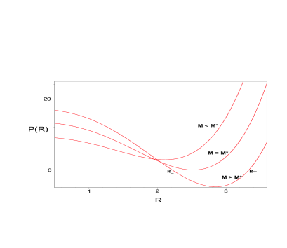
Figure 1: The polynomial $P(R)\equiv R^{4}g_{TT}$ for dust masses $M<M_{\ast}$ (no event horizon), $M=M_{\ast}$ (extremal black hole) and $M>M_{\ast}$ (black hole formation with a event horizon ${R}_{+}$ and a Cauchy horizon ${R}_{-}$). We consider here $|\sigma|=0.05$, in units $G_{N}=c=1$.

In this case the collapse of the surface of dust must cross ${R}_{-}$ , that is, $\gamma a_{m}<{R}_{-}$  so that a stable black hole forms with trapped perpetually bouncing matter.

Let us then consider the following coordinates transformation

$$\frac{2\kappa}{u}du:=\frac{R^{4}}{P(R)}dR-dT,$$ (34)

$$\frac{2\kappa}{v}dv:=\frac{R^{4}}{P(R)}dR+dT.$$ (35)

Therefore, from (2) we get

$$ds^{2}=\frac{4\kappa^{2}}{uv}\frac{P(R)}{R^{4}}dudv+R^{2}(d{\theta}^{2}+\sin^{2}{{\theta}}d{\phi}^{2}).$$

By defining

$$R^{\ast}:=\int g_{RR}dR,$$ (36)

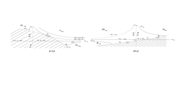
Figure 2: Kruskal diagrams showing the curve ABCD which illustrates how the matter surface evolves in time. The shaded portion corresponds to the interior of the matter distribution. Figures (a) and (b) overlap in the region $II_{b}$, and may be regarded as linked together along the curve $R=R_{0}$, where $R_{0}$ is any convenient value between $R_{+}$ and $R_{-}$.

we get that

$$R^{\ast}=R+G\ln{\Big{|}\frac{R}{R_{+}}-1\Big{|}}+W\ln{\Big{|}\frac{R}{R_{-}}-1\Big{|}}~{}~{}~{}~{}~{}~{}~{}~{}~{}~{}~{}~{}$$

$$+\frac{2J}{\sqrt{4\beta-\alpha^{2}}}\arctan{\Big{(}\frac{2R+\alpha}{\sqrt{4\beta-\alpha^{2}}}\Big{)}},$$ (37)

where

$$G := \frac{R^{4}_{+}}{(R_{+}-R_{-})(R^{2}_{+}+\alpha R_{+}+\beta)}~{}~{},~{}~{}$$ (38)

$$W := -\frac{R^{4}_{-}}{(R_{+}-R_{-})(R^{2}_{-}+\alpha R_{-}+\beta)}~{}~{},$$ (39)

$$J := \beta\Big{(}\frac{A}{R_{+}}+\frac{B}{R_{-}}-1\Big{)}.~{}~{}$$ (40)

Therefore, integration of (34) and (35) yields

$$R^{\ast}=\kappa\ln|uv|~{}~{},~{}~{}T=\kappa\ln|v/u|.$$ (41)

Consider now the chart $(u_{1},v_{1})$ (defined for $R>R_{-}$) obtained by setting $\kappa=G$. From (3) and (38) we find that

$$u_{1}v_{1}=\Big{(}\frac{R}{R_{+}}-1\Big{)}\Big{(}\frac{R}{R_{-}}-1\Big{)}^{-\frac{|W|}{G}}~{}~{}~{}~{}~{}~{}~{}~{}~{}~{}~{}~{}~{}~{}~{}~{}~{}~{}~{}~{}~{}~{}~{}~{}~{}~{}~{}~{}$$

$$\times\exp{\Big{[}\frac{R}{G}+\frac{2J}{G\sqrt{4\beta-\alpha^{2}}}\arctan{\Big{(}\frac{2R+\alpha}{\sqrt{4\beta-\alpha^{2}}}\Big{)}}\Big{]}}.$$ (42)

and (3) exhibits no singularity at $R=R_{+}$. The chart $(u_{1},v_{1})$ in fact gives a regular mapping of any given subregion of the manifold which has $R>R_{-}$. However, a coordinate singularity does develop at $R=R_{-}$ and it is necessary to go over another chart before that happens.

Define the chart $(u_{2},v_{2})$ (defined for $R<R_{+}$) by setting $\kappa=B$. From (3) and (38) we find that

$$u_{2}v_{2}=\Big{(}1-\frac{R}{R_{+}}\Big{)}^{-\frac{G}{|W|}}\Big{(}\frac{R}{R_{-}}-1\Big{)}~{}~{}~{}~{}~{}~{}~{}~{}~{}~{}~{}~{}~{}~{}~{}~{}~{}~{}~{}~{}~{}~{}~{}~{}~{}~{}~{}$$

$$\times\exp{\Big{[}\frac{R}{W}+\frac{2J}{W\sqrt{4\beta-\alpha^{2}}}\arctan{\Big{(}\frac{2R+\alpha}{\sqrt{4\beta-\alpha^{2}}}\Big{)}}\Big{]}},$$ (43)

and this provides a regular covering for any subregion with $R<R_{+}$.

In the domain of overlap $R_{-}<R<R_{+}$ the two charts are related by

$$|u|^{G}_{1}=|u|^{W}_{2}~{}~{},~{}~{}|v|^{G}_{1}=|v|^{W}_{2}.$$ (44)

Figures 2(a), 2(b) are Kruskal-type diagrams which together give a faithful map of any subregion covered by a pair of overlapping charts $(u_{1},v_{1})$ and $(u_{2},v_{2})$. The maximal analytical extension of spacetime (2) is analogous to that of a Reissner-Nordström black hole[1, 23] with an exterior event horizon $R_{+}$ and a Cauchy horizon $R_{-}$ (cf. Fig. 3).

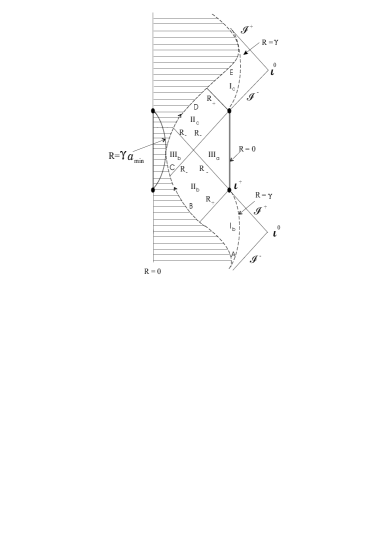
Figure 3: Penrose diagram for the spacetime assuming $M>M_{\ast}$. The infinite chain of asymptotically flat regions I $(\infty>R>R_{+})$ are connected to regions III $(R_{-}>R>\gamma a_{min})$ by regions II $(R_{+}>R>R_{-})$. The shaded portion, limited by $R=\gamma a_{min}$ and $R=\gamma$ corresponds to the interior of the matter distribution. The same dotted line ABCDE illustrates how the matter surface evolves in time. Once crossed $R_{-}$ such a surface keeps bouncing between $R=\gamma$ and $R=\gamma a_{min}$.

Here the singularity in the interior of the matter distribution is barred by the timelike surface $R=\gamma a_{m}$ where the spacetime extension ends.

By taking $M_{\ast}$ as the maximum value for a white dwarf to be in equilibrium ($1.4M_{\bigodot}$), we have that the domain for the brane tension is given by the lower limit

$$|\sigma|\gtrsim 10^{-8}\frac{1}{m^{2}}.$$

In fact, the behavior of the $S$ function does not change when $|\sigma|>10^{-7}\frac{1}{m^{2}}$. Therefore we justify the typical value $|\sigma|=0.05$ adopted in our numerical illustration in Sec. 2.

4 The Hawking Temperature

In 1975, S. W. Hawking derived – through a semi-classical approach – the thermal spectrum of emitted particles by a black hole.[24] In this Section we are going to follow this same original procedure in order to derive the corrections in the Hawking radiation.

Let us consider a massless Klein-Gordon field $\varphi$ in the background defined by the exterior spacetime (2). The propagation of such scalar test field is taken to be governed by the scalar wave equation

$$g^{ab}\nabla_{a}\nabla_{b}~{}\varphi=0.$$ (45)

Exploiting the symmetries of the background we seek a solution as

$$\varphi_{\omega ml}=\frac{1}{R}R_{\omega l}(R^{\ast})Y_{ml}(\theta,\phi)\exp(-i\omega t).$$ (46)

Substituting this expression for $\varphi$, the wave equation is reduced to an ordinary differential equation in $R^{\ast}$ for the modes $R_{\omega l}$ and given by

$$\frac{d^{2}R_{\omega l}}{d{R^{\ast}}^{2}}+\Big{\{}\omega^{2}-\frac{1}{R^{2}}\Big{[}l(l+1)+\frac{2G_{N}M}{R}-\frac{3G_{N}M^{2}}{\pi|\sigma|R^{4}}\Big{]}~{}~{}~{}~{}~{}~{}~{}~{}~{}~{}~{}~{}~{}~{}~{}~{}$$

$$\Big{(}1-\frac{2G_{N}M}{R}+\frac{3G_{N}M^{2}}{4\pi|\sigma|R^{4}}\Big{)}\Big{\}}R_{\omega l}=0.$$ (47)

As $r\rightarrow\pm\infty$ we have that

$$\frac{d^{2}R_{\omega l}}{d{R^{\ast}}^{2}}+\omega^{2}R_{\omega l}=0\Rightarrow R_{\omega l}(R^{\ast})=\exp(\pm i\omega{R^{\ast}})$$

and, asymptotically, one can express the Klein Gordon field as

$$\varphi_{1}=\frac{1}{R}\exp[-i\omega(t-{R^{\ast}})]Y_{ml}(\theta,\phi)$$ (48)

and

$$\varphi_{2}=\frac{1}{R}\exp[-i\omega(t+{R^{\ast}})]Y_{ml}(\theta,\phi).$$ (49)

Let us now assume that the source that generates the exterior solution (2) is given by a thin shell of a spherically symmetric matter distribution, and the flat spacetime inside such distribution is given by

$$ds^{2}=-dt^{2}+dr^{2}+r^{2}d\Omega^{2}.$$ (50)

Defining $a(t)$ as the scale factor that the describes the evolution of the matter distribution, we impose that the interior metric match the exterior geometry by the following equation

$$1-\Big{(}\frac{da}{dt}\Big{)}^{2}=\Big{(}1-\frac{2G_{N}M}{a}+\frac{3G_{N}M^{2}}{4\pi|\sigma|a^{4}}\Big{)}\Big{(}\frac{dT}{dt}\Big{)}^{2}~{}~{}~{}~{}~{}~{}~{}~{}~{}~{}~{}~{}~{}~{}~{}~{}~{}~{}$$

$$-\Big{(}1-\frac{2G_{N}M}{a}+\frac{3G_{N}M^{2}}{4\pi|\sigma|a^{4}}\Big{)}^{-1}\Big{(}\frac{da}{dt}\Big{)}^{2}.$$ (51)

We also define the respective null interior and exterior coordinates by

$$V:=t+r~{},~{}~{}U:=t-r~{},$$ (52)

and

$$v:=T+R^{\ast}~{},~{}~{}u:=T-R^{\ast}.$$ (53)

Let us now assume that the null incident rays get into the matter distribution when $a=a_{I}\gg R_{+}\sim GM$. Therefore we have that

$$\Big{(}1-\frac{2G_{N}M}{a_{I}}+\frac{3G_{N}M^{2}}{4\pi|\sigma|{a_{I}}^{4}}\Big{)}\rightarrow 1.$$ (54)

and

$$\Big{(}\frac{dT}{dt}\Big{)}^{2}\simeq 1\rightarrow t\simeq T.$$ (55)

On the other hand,

$$v_{I}\simeq t+R^{\ast}\Rightarrow V_{I}=v_{I}+\kappa$$ (56)

where

$$\kappa=a_{I}-R^{\ast}(a_{I}).$$ (57)

When $r=0$, we derive the trivial relation between $V$ and $U$ at the center of the matter distribution:

$$V_{0}=t=U_{0}.$$ (58)

Let us now consider that the outgoing waves emerge from the matter distribution when $a=a_{II}\sim R_{+}$. If $t_{0}$ is taken to be the instant in which $a=R_{+}$, one may expand the scale factor $a_{II}(t)$ in Taylor series as

$$a_{II}(t)\simeq R_{+}+F(t_{0}-t),$$ (59)

where F is a constant.

Therefore, from equation (4) we have

$$T\simeq-\lambda\ln(t_{0}-t)$$ (60)

up to first order in $(t_{0}-t)$, where

$$\lambda\equiv\frac{\sqrt{2G_{N}MR^{3}_{+}-3G_{N}M^{2}/4\pi|\sigma|}}{4R_{+}-6G_{N}M}.$$ (61)

However, from (3) we have

$$R^{\ast}\simeq G\ln{\Big{(}\frac{a}{R_{+}}-1\Big{)}}.$$ (62)

Then we get

$$u_{II}\simeq-\delta\ln{(t_{0}-t)},$$

where $\delta\equiv\lambda+G$. Therefore,

$$U_{II}\simeq\chi\exp{\Big{(}-\frac{u_{II}}{\delta}\Big{)}}+\psi$$ (63)

where

$$\chi=-(1+F)~{},~{}~{}\psi=t_{0}-R_{+}.$$ (64)

However, at the origin of the coordinate system we have $U_{0}=V_{0}$. Therefore the relation between the exterior null coordinates is given by

$$v=v_{0}+\chi\exp{\Big{(}-\frac{u}{\delta}\Big{)}}~{},~{}~{}u=-\delta\ln{\Big{(}\frac{v-v_{0}}{\chi}\Big{)}}$$ (65)

where

$$v_{0}:=\psi-\kappa.$$ (66)

Using (49) we expand $\varphi_{1\omega lm}$ in terms of $\varphi_{2\omega lm}$ as

$$\varphi_{1\omega lm}=\int^{\infty}_{0}[\alpha^{\ast}_{\omega^{\prime}\omega lm}\exp{(-i\omega^{\prime}v)}-\beta_{\omega^{\prime}\omega lm}\exp{(i\omega^{\prime}v)}]d\omega^{\prime},$$

where $\alpha^{\ast}_{\omega^{\prime}\omega lm}$ and $\beta_{\omega^{\prime}\omega lm}$ are the Bogolubov coefficients.[25] Therefore, it is straightforward to show[24] that

$$|\alpha_{\omega^{\prime}\omega lm}|=\pi\omega\delta|\beta_{\omega^{\prime}\omega lm}|.$$ (67)

However, it follows from the orthogonality propriety of $\varphi_{1\omega lm}$ and $\varphi_{2\omega lm}$ that

$$\sum_{\omega^{\prime}}[~{}|\alpha_{\omega^{\prime}\omega lm}|^{2}-|\beta_{\omega^{\prime}\omega lm}|^{2}~{}]=1.$$ (68)

Therefore we obtain that the spectrum of the average number of created particles on the $\omega lm$ mode is given by

$$N_{\omega lm}=\sum_{\omega^{\prime}}|\beta_{\omega^{\prime}\omega lm}|^{2}=\frac{1}{\exp{(2\pi\delta\omega)}-1}.$$ (69)

The above result corresponds to a Planckian spectrum with associated temperature

$$T_{H}=\frac{\Big{(}R_{+}-R_{-}\Big{)}}{2\pi R_{+}~{}\zeta},$$ (70)

where

$$\zeta=\frac{R_{+}^{3}}{(R_{+}^{2}+\alpha R_{+}+\beta)}+\Big{[}\frac{\sqrt{3G_{N}M~{}(2R_{+}^{3}-M/4\pi|\sigma|)}(R_{+}-R_{-})}{{2R_{+}(2R_{+}-3G_{N}M)}}\Big{]}.$$ (71)

The Hawking temperature depends on the parameters $M$ and $|\sigma|$. We note that in the extremal case we have $R_{+}=R_{-}=3G_{N}M/2$ implying that $T_{H}\rightarrow 0$ continuously as $R_{+}\rightarrow R_{-}$. The observation of Hawking radiation could, in principle, allows us to test our results for finite $|\sigma|$. Another feature, which demands a carefully analysis, is related to the entropy. We dedicate Sec. 5 to this subject.

5 Black Hole Thermodynamics and the Quest for a Statistical Mechanics Model for the Entropy of Quasi-extremal Black Holes

Motivated by the analysis of energy processes involving black holes Bekenstein[26] made the remarkable assumption that the entropy of a black hole should be proportional to the area of its event horizon and formulated a First Law of Black Hole Thermodynamics where the surface gravity of the black hole appeared as proportional (via dimensional fundamental constants) to a temperature. Bekenstein’s results however did not involve any fundamental principle of statistical mechanics. Two years later S. W. Hawking,[24] by examining the quantum creation of particles near a Schwarzschild black hole, showed that the black hole emits particles with a Planckian thermal spectrum of temperature $T_{BH}=\kappa/2\pi$ (in units $\hbar=c=G_{N}=K_{B}=1$) where $\kappa=1/4M$ is the surface gravity of the black hole. This striking result fits exactly in the Bekenstein formula for the First Law of black hole thermodynamics, thus validating Bekenstein’s proposals and fixing the proportionality factor connecting the entropy and the area of the black hole.

Nevertheless by considering the classical theory of General Relativity, the singularity issue still posed an insurmountable barrier to the task of constructing a model for the interior of the black hole and of counting its degrees of freedom, what would eventually lead to a definition of entropy.

The results of the geometrical Black Hole Thermodynamics of Bekenstein are recovered in our model for the case of quasi-extremal black holes with an additional term connected to the work done by the variation of the brane tension. Let us consider a small deviation from the extremal case, with $R_{\pm}=\frac{3G_{N}M}{2}\pm\epsilon$ where $\epsilon$ is infinitesimal. Neglecting higher order terms in $\epsilon$ we have from $P(R_{\pm})=0$ that

$$\epsilon=\sqrt{\frac{3G^{2}_{N}M^{2}}{8}-\frac{1}{6\pi G_{N}|\sigma|}},$$ (72)

from which the useful relation is derived,

$$d\epsilon\simeq\frac{1}{2\epsilon}\Big{(}\frac{3G_{N}^{2}M_{\ast}}{4}~{}dM+\frac{1}{6\pi G_{N}|\sigma_{\ast}|^{2}}~{}d|\sigma|\Big{)},$$ (73)

and which is valid about the extremal configuration. The condition for horizon formation is given by $\epsilon\geq 0$.

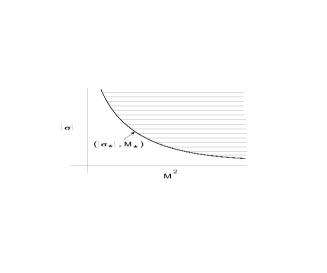
Figure 4: The parameter space ($|\sigma|,M^{2}$): the shaded area corresponds to black hole configurations with two horizons; the white area corresponds to configurations with no black hole formation. The condition $\epsilon=0$ defines the limiting curve ($|\sigma_{\ast}|,M_{\ast}$) that corresponds to extremal black hole configurations. The region that we are considering here is given by sufficiently large values of $|\sigma|$, and very near the extremal curve on the shaded side.

The equality in this latter relation defines a curve (cf. Fig. 4) in the parameter space ($|\sigma|,M^{2}$) that corresponds to extremal black holes. The region above the curve is the region of black holes (with two horizons) while the region below defines configurations with no horizon formation and therefore no black holes. In this sense, $\epsilon$ corresponds to a small deviation from the curve ($|\sigma_{\ast}|,M_{\ast}$) towards the black hole area of the parameter space. In this approximation the Hawking temperature is small and given by

$$T_{H}\simeq\Big{(}\frac{8\hbar}{9\pi K_{B}G^{2}_{N}M^{2}_{\ast}}\Big{)}~{}\epsilon,$$ (74)

where we now restore the constants $\hbar$ and $K_{B}$. By defining the the outer horizon area as $A_{\rm outer}:=4\pi R^{2}_{+}\simeq\Big{(}A_{\rm extr}+12\pi G_{N}M_{\ast}\epsilon\Big{)}$, we obtain for the quasi-extremal case that

$$\frac{K_{B}}{4G_{N}\hbar}dA_{\rm outer}\simeq\frac{1}{T_{H}}\Big{(}dM+\frac{M_{\ast}}{2|\sigma_{\ast}|}d|\sigma|\Big{)}.$$ (75)

where Eq. (73) has been used. We can therefore associate the horizon area of the quasi-extremal black hole with the geometrical entropy

$$S_{geom}=\frac{K_{B}}{4G_{N}\hbar}A_{\rm outer},$$ (76)

a result which is in accordance to Bekenstein’s definition.[26] Equation (75) is an extended First Law with an extra work term connected to the variation of the brane tension. For deviations with $|\sigma|={\rm const.}$ we recover the form of the First Law for the Schwarzschild black hole in the brane scenario.

We are now led to tentatively construct a statistical mechanics model for the bouncing collapsed matter (in the quasi-extremal case) with an associated partition function engendering a thermodynamics which, under certain assumptions, may be connected to the geometrical thermodynamics discussed above. The following facts about the quasi-extremal configurations are fundamental to our approach. The quasi-extremal configurations are basically characterized by the parameter $\epsilon$ (cf. Eq. (72)) that fixes not only the oscillatory motion of the collapsed matter but also all the properties of the extended spacetime, in particular determining the geometrical thermodynamic variables of the exterior spacetime. Actually $\epsilon$ is a measure of all the fluctuations about the extremal case, either occurring in the dynamics of the oscillating collapsed matter or determining the horizon fluctuations of the exterior geometry.

To proceed let us consider the dynamical equation for the scale factor expressed by the constraint (15), with the initial conditions $\dot{a}(0)=0$ and $a(0)=1$. Once the surface of matter distribution is defined by $R\equiv\gamma a$, we can define the momentum (per unity of mass) at the surface distribution as $p_{R}:=\gamma~{}\dot{a}$ so that the dynamical equation for the scale factor is given by the Hamiltonian constraint

$$H=\Big{[}\frac{p^{2}_{R}}{2}+V(R)\Big{]}=0,$$ (77)

where

$$V(R):=\frac{3G_{N}M^{2}}{8\pi|\sigma|R^{4}}-\frac{G_{N}M}{R}+\frac{k\gamma^{2}}{2}.$$

Expanding (77) in a neighborhood of $R=R_{\ast}=3G_{N}M_{\ast}/2$ (the extremal configuration) we obtain

$$\mathcal{H}:=\frac{p^{2}_{R}}{2}+\frac{4}{9G^{2}_{N}M_{\ast}^{2}}\Big{[}\frac{8}{3G_{N}M_{\ast}}\epsilon^{2}R+\Big{(}1-\frac{40}{9G^{2}_{N}M^{2}_{\ast}}\epsilon^{2}\Big{)}R^{2}\Big{]}\simeq-V(R_{\ast}).~{}~{}~{}~{}$$ (78)

As the brane formulation must approach General Relativity in the low energy limit, it is natural to expect the value of $|\sigma_{\ast}|$ to be sufficiently large. In this instance the brane tension satisfies the inequality $\sqrt{1/(3\pi G_{N}|\sigma_{\ast}|)}\ll 1$, which implies that the term proportional to $R$ in (78) can be neglected. The constraint (78) is then approximately given by

$$H=\frac{p^{2}_{R}}{2}+\frac{1}{2}\omega^{2}R^{2}\simeq-V(R_{\ast}),$$ (79)

where

$$\omega\equiv\frac{2\sqrt{2}}{3G_{N}M_{\ast}}\sqrt{\Big{(}1-\frac{40}{9G^{2}_{N}M_{\ast}^{2}}\epsilon^{2}\Big{)}}\simeq\frac{2\sqrt{2}}{3G_{N}M_{\ast}}-\frac{40\sqrt{2}}{27G^{3}_{N}M_{\ast}^{3}}\epsilon^{2}.$$ (80)

As we are assuming a non-interacting fluid, the interior particles of the matter distribution must also oscillate with a frequency $\omega$. We should note that the first term in the second equality of (80) corresponds to the oscillation of the matter distribution in the extremal case, which is thermodynamically a configuration of zero temperature, while the second term corresponds to oscillations generated by small deviations from the extremal configuration which depend on the parameter $\epsilon$. This same parameter is responsible for horizon fluctuations about the extremal case which give rise to the geometrical Hawking temperature associated with the exterior spacetime, as seen from (74). In analogy with the result (74) of the Hawking temperature, we make the provisional assumption that the second term in (80) arises from fluctuations which we denote thermal, connected to a temperature $T_{S}$ given by

$$T_{S}:=a~{}\Big{(}\frac{8\hbar}{9\pi K_{B}G^{2}_{N}M^{2}_{\ast}}\Big{)}~{}\epsilon,$$ (81)

where $a$ is an adimensional constant. In this sense, from the point of view of statistical mechanics, the extremal configuration would obviously have a zero partition function, being a zero temperature configuration. However this is not the case in the quasi-extremal cases for which a partition function can be constructed by quantizing the thermal fluctuations appearing (80) as we proceed to show.

Let us define $N_{\ast}$ as the number of Planck masses contained in the matter of the extremal case, $N_{\ast}=M_{\ast}/m_{\rm Pl}$. The approximated motion of our system can then be interpreted as the 1-dim motion of $N_{\ast}$ noninteracting oscillators with frequency $\omega$, the energy levels of which – under a quantization procedure – will be given by $E_{n}=(n+1/2)\hbar\omega$. The fluctuations about the extremal configuration present in $\omega$ and now parametrized with the temperature $T_{S}$ will engender quantum thermal fluctuations that will have a fundamental contribution in the partition function.

The canonical partition function of the system may then be expressed as

$$Z=\Big{\{}\sum^{\infty}_{n=0}\exp\Big{[}-\Big{(}n+\frac{1}{2}\Big{)}\beta\hbar\omega\Big{]}\Big{\}}^{N_{\ast}}=\Big{[}\frac{\exp(\beta\omega\hbar/2)}{\exp(\beta\omega\hbar)-1}\Big{]}^{N_{\ast}}$$

$$\simeq{\rm exp}(-N_{\ast}\beta\omega\hbar/2),~{}$$ (82)

where $\beta\equiv 1/K_{B}T_{S}$ and the third equality results from $T_{S}$ being small for the quasi-extremal case.

The free energy is given by

$$F=-{\cal R}~{}T_{S}\ln{Z}\simeq\frac{N_{\ast}{\cal R}\omega\hbar}{2K_{B}},$$ (83)

where ${\cal R}$ is an appropriate constant. By definition the entropy of the system can be calculated as a function of the free energy through the relation $S=-{\partial F}/{\partial T_{S}}$, resulting in

$$S_{stat}\simeq\frac{40\sqrt{2}N_{\ast}{\cal R}\hbar}{27K_{B}G^{3}_{N}M^{3}_{\ast}a^{2}}T_{S}=\frac{5\sqrt{2}\pi N_{\ast}{\cal R}}{3G_{N}M_{\ast}a}~{}\epsilon,$$ (84)

where use was made of Eq. (81). Therefore, using the relations (72)-(73), we obtain

$$dS_{stat}\simeq\frac{1}{T_{S}}\Big{(}dM+\frac{M_{\ast}}{2|\sigma_{\ast}|}d|\sigma|\Big{)},$$ (85)

where we have fixed ${\cal R}:=K_{B}\tilde{N}$, with $\tilde{N}=\frac{9\sqrt{2}}{10}N_{\ast}\simeq 1.272N_{\ast}$. We see that $\tilde{N}$ arises naturally as the analog of an Avogadro number for the internal matter distribution of the extremal case. Also Eq. (85), which is a first law of thermodynamics for the bouncing collapsed matter, validates our definition (81) of $T_{S}$ as a temperature.

By comparing Eqs. (75) and (85) we are led to identify $T_{S}$ with the Hawking temperature $T_{H}$ which was derived in Section 4 for the exterior spacetime, therefore fixing $a=1$ in (81). We should remark that the statistical entropy derived in (84) differs from Bekenstein’s entropy $S_{geom}$ (76) by a zero temperature additive constant which corresponds to the area of the extremal black hole about which our treatment is made, namely

$$S_{geom}=\frac{K_{B}}{4\hbar G_{N}}A_{extr}+S_{stat}~{}.$$ (86)

In fact we can see that the statistical entropy (84) arises just from the quantum thermal fluctuations with which the partition function is built, in distinction to the geometrical entropy of Bekenstein.

Notwithstanding these striking similarities, a question that can now be posed is how the concepts of Hawking temperature and Bekenstein entropy can be connected with the above defined entropy and temperature of the interior bouncing matter. In fact, in accordance with the geometrical black hole thermodynamics, one might argue that the entropy of the black hole is an external variable connected to the event horizon boundary of the exterior gravitational field. Therefore the entropy of the collapsed matter would thus be irrelevant for physical processes outside the black hole. However, as far as quasi-extremal configurations are considered, we can suggest a mechanism of how the quantum thermal fluctuations may connect the entropy of the collapsed matter to fluctuations of the outer event horizon. To see this, let us consider the fundamental frequency $\Delta\omega$, of a particle of the oscillating matter distribution with mass $m_{pl}$, given by (cf. (80))

$$\Delta\omega=\frac{40\sqrt{2}}{27G^{3}_{N}M_{\ast}^{3}}\epsilon^{2}.$$ (87)

Its associated momentum is given by $\Delta p=\sqrt{2\hbar m_{pl}\Delta\omega}$. According to Heisenberg uncertainty principle the uncertainty in its localization $\Delta R\geq\hbar/2$ and, using (87), we obtain

$$\Delta R\geq\frac{1}{2\epsilon}\sqrt{\frac{27G^{3}_{N}M_{\ast}^{3}\hbar}{40\sqrt{2}~{}m_{Pl}}}.$$ (88)

For illustration, by taking $M_{\ast}$ as the Chandrasekhar mass ($M_{\ast}=1.4M_{\odot}$) we find $\Delta R\geq 0.4127626961\times 10^{-14}m^{2}/\epsilon$. On the other hand $R_{+}\sim 3G_{N}M_{\ast}/2=3\times 10^{3}m$. Therefore, if $\epsilon\lesssim 10^{-18}m$, namely smaller than $10^{17}l_{P}$ (where $l_{P}$ is the Planck length), we can assure that the scale of the fluctuations $\Delta R>R_{+}$ so that the quantum thermal fluctuations that give rise to the entropy (84) of the collapsed matter might be connected to the fluctuations of the event horizon in the quasi-extremal case. In this sense, Eqs. (75) and (85) validate the identification of both entropies (up to an additive constant corresponding to the area of the extremal black hole) with the proviso that the temperature responsible for the thermal fluctuations is identified with the Hawking temperature.

An extension of our analysis beyond the quasi-extremal approximation will be the subject of a future work. In this instance the collapsed matter distribution should be strongly correlated and its description as noninteracting oscillating particles should be drastically modified.

6 Conclusions and Final Comments

In this paper we have examined the gravitational collapse of pure dust in a braneworld scenario. By considering a timelike extra dimension of the bulk we show that the classical singularity produced by the collapse can be avoided, resulting instead in a bouncing nonsingular solution. For the case of the total mass $M$ of the collapsing dust greater than a critical value $M_{\ast}$ (which depends on the brane tension) the smooth junction of this solution with the exterior geometry results in a spacetime analogous to the Reissner-Nordström geometry, with an exterior event horizon and a Cauchy horizon which enclose the collapsed bouncing matter. We construct the analytical extension of the spacetime up to the surface of the bouncing collapsed matter where the two geometries are smoothly connected. For $M=M_{\ast}$ we have the extremal black hole configuration with one horizon only. This case plays a fundamental role in our discussion of possible entropy definitions for the system.

In the case of $M>M_{\ast}$, the effects of the bulk-brane corrections on the classical observational tests of General Relativity were calculated but not included in the paper. However for completeness some of these results are briefly commented in the following. To start let us note that the dynamics of General Relativity is recovered in the limit $|\sigma|\rightarrow\infty$. Concerning the advance of the planetary perihelion, due to the brane-bulk corrections in the geometry, the perihelion precession per revolution decreases when compared to the predicition of General Relativity, for the present case of a timelike extra dimension. On the contrary, for a spacelike extra dimension, the perihelion precession increases. In both cases the observational data[27] restrict the brane tension $|\sigma|$ to be greater than $10^{-8}{m^{-2}}$.

Analogously for the bending of light rays passing in the neighborhood of a spherical massive body, the effects predicted by General Relativity are attenuated due to the corrections in the case of a timelike extra dimension. In the case of a spacelike extra dimension the deflection angle of the asymptotes increases. It is worth remarking that the observational data[28] do not impose a new limit for the brane tension. In fact, in this case we only need that $|\sigma|\geq 10^{-12}m^{-2}$ for both cases of a timelike or spacelike extra dimension. Summarizing the effects of the bulk-brane corrections on the classical tests of General Relativity are attenuated (increased) when one considers a timelike (spacelike) extra dimension. Although the predictions of General Relativity are corroborated by the observational tests in the solar system, the corrections of our model may turn out to be significative when we consider higher energy and/or curvature scales.

The central result of our work is contained in Secs. $4$ and $5$. In Sec. 4 we calculated (through a semiclassical approach) of the corrected Hawking temperature in our model. We also obtain that, analogous to the case of General Relativity, we have the prediction of a zero temperature for the case of extremal black holes. The calculation of the modified Hawking temperature allowed us to derive, analogously to Bekenstein, a geometric entropy that confirms (for quasi-extremal black holes) the classical prediction that the entropy is proportional to the area of the event horizon, as shown in the first part of Sec. $5$. Although the classical black hole thermodynamics introduced by Bekenstein was validated by Hawking’s semiclassical derivation of the black body thermal emission of a black hole, with a temperature proportional the the gravity surface of the event horizon of the black hole, black hole thermodynamics always seemed to possess a heuristic character since no basic principle of statistical mechanics was used in its derivation. Indeed, the definition of the entropy of black holes is still an open problem and we actually refer to it as a geometrical entropy.

In this context, in the remaining of Sec. $5$, we have tentatively constructed a simple statistical mechanics model for the entropy of the oscillatory collapsed matter in the case of quasi-extremal black holes. In fact, by quantizing the internal degrees of freedom of the quasi-extremal configuration, we constructed a statistical partition function and a free energy – and assuming that the temperature responsible for the thermal fluctuations obeys the same form of the Hawking temperature – we derive an entropy that satisfies a first law of thermodynamics strikingly similar to the geometrical first law for the quasi-extremal black hole. This statistical entropy differs from Bekenstein’s entropy by a zero temperature additive constant which corresponds to the area of the extremal black hole about which our treatment is made. In fact we can see that the statistical entropy arises from the quantum thermal fluctuations with which the partition function is built, in distinction to the geometrical entropy of Bekenstein.

We should finally mention that the presence of the Cauchy horizon $R_{-}$ in the maximal analytical extension of the geometry (2) may pose the question of a possible instability of the spacetime as measured by geodetic observers.[1] We are aware that this may constitute a problem to our statistical treatment of the bouncing collapsed matter, but not to the geometrical entropy formation of Sec. 6 for the exterior spacetime. We intend to approach this issue in a future publication.

7 Acknowledgements

The authors acknowledge the partial financial support of CNPq/MCTI-Brazil.

References

- [1] S. Chandrasekhar, The Mathematical Theory of Black Holes (Oxford University Press, New York, 1983).
- [2] W. Israel, Phys. Rev. 164 (1967) 1776.
- [3] B. Carter, Phys. Rev. Lett. 26 (1971) 331.
- [4] R. M. Wald, General Relativity (University of Chicago Press, Chicago, 1984).
- [5] J. R. Oppenheimer and H. Snyder, Phys. Rev. 56 (1939) 455.
- [6] R. Penrose, Phys. Rev. Lett. 14 (1965) 57.
- [7] M. Bojowald, R. Goswami, R. Maartens and P. Singh, Phys. Rev. Lett. 95 (2005) 091302.
- [8] L. Randall and R. Sundrum, Phys. Rev. Lett. 83 (1999) 4690.
- [9] Y. V. Shtanov. Phys. Lett. B 541 (2002) 177.
- [10] Y. V. Shtanov and V. Sahni, Phys. Lett. B 557 (2003) 1.
- [11] T. Shiromizu, K. Maeda and M. Sasaki, Phys. Rev. D 62 (2000) 024012.
- [12] R. Maartens, Phys. Rev. D 62 (2000) 084023.
- [13] R. Maartens Living Rev. Rel. 7 (2004) 7.
- [14] M. Bruni, C. Germani, and R. Maartens, Phys. Rev. Lett. 87 (2001) 231302.
- [15] N. Dadhich, R. Maartens, P. Papadopoulos and V. Rezania, Phys. Lett. B 487 (2000) 1.
- [16] M. Govender and N. Dadhich, Phys. Lett. B 538 (2002) 233.
- [17] N. Dadhich and S. G. Ghosh, Phys. Lett. B 518 (2001) 1.
- [18] R. Maier and F. T. Falciano, Phys. Rev. D 83 064019 (2011).
- [19] L. P. Eisenhart, Riemannian Geometry (Princeton University Press, New Jersey, 1997).
- [20] A. H. Taub, Phys. Rev. 94 (1954) 6.
- [21] W. Israel, Nuovo Cimento A 44 (1966) 1.
- [22] S. Weinberg, Gravitation and Cosmology (John Wiley & Sons, Inc., 1972).
- [23] V. de La Cruz and W. Israel, Nuovo Cimento A 51 (1967) 3.
- [24] S. W. Hawking, Commun. Math. Phys. 43 (1975) 199.
- [25] N. D. Birrel and P. C. Davies, Quantum Fields in Curved Spacetimes (Cambridge University Press, Cambridge, 1982).
- [26] Jacob. D. Bekenstein, Phy. Rev. D 7 (1973) 2333.
- [27] G. M. Clemence, Rev. Mod. Phys. 19 (1947) 361.
- [28] F. W. Dyson, A. S. Eddington and C. Davidson, Mem. R. Astron. Soc. 62 (1920) 291.