Topological entanglement entropy in Gutzwiller projected spin liquids

Abstract

The topological entanglement entropy(TEE) of Gutzwiller projected RVB state is studied with Monte Carlo simulation. New tricks are proposed to improve the convergence of TEE, which enable us to show that the spin liquid state studied in Ref.Vishwanath actually does not support $Z_{2}$ topological order, a conclusion that is consistent with the information drawn from the inspection of the topological degeneracy on the same state. We find both a long ranged RVB amplitude and an approximate Marshall sign structure are at the origin of the suppression of vison gap in this spin liquid state. On the other hand, robust signature of $Z_{2}$ topological order, i.e., a TEE of $\ln 2$, is clearly demonstrated for a Gutzwiiler projected RVB state on triangular lattice which is evolved from the RVB state proposed originally by AndersonSorella . We also find that it is the sign, rather than the amplitude of the RVB wave function, that dominates the TEE and is responsible for a positive value of TEE, which implies that the nonlocal entanglement in the RVB state is mainly encoded in the sign of the RVB wave function. Our results indicate that some information that is important for the topological property of a RVB state is missed in the effective field theory description and that a $Z_{2}$ gauge structure in the saddle point action is not enough for the RVB state to exhibit topological order, even if its spin correlation is extremely short ranged.

I I.Introduction

The search for spin liquid phases in quantum antiferromaget is a hot topic in the field of strongly correlated electron systemsFrustrated . A spin liquid state is an exotic state of matter in that it can exhibit novel structures and excitations beyond the Landau-Ginzburg paradigm. The topological order and the related fractionalized excitation are one of such possibilities. A topological ordered system is unique in that its ground state exhibits topological degeneracy on multiply connected manifolds. A topological ordered state is also associated with a nonzero topological contribution to the entanglement entropyKitaev ; Levin .

Following the original idea of resonating valence bond state, two approaches are widely used for the description of spin liquid phase. The first one is the effective field theory approach based on slave particle representation of the spin degree of freedomLee . The second one is the variational approach based on Gutzwiller projected wave functionsSorella . The Gutzwiller projection procedure, which removes the doubly occupied configuration in the mean field ground state, amounts to perform gauge averaging on the saddle point of the effective field theory. Thus, if the gauge fluctuation is irrelevant in the long wavelength limit, one should expect the Gutzwiller projected RVB state to exhibit the same long range physics as the effective field theory. In a gapped spin liquid, the only nontrivial physics in the long wavelength limit is its topological property. However, it is found earlier that the topological property predicted by the effective field theory does not always agree with that found from the corresponding Gutzwiller projected wave function. In particular, the Marshall sign rule is found to be closely related to the the absence of the topological order in certain spin liquid statesLi1 ; Li2 ; Li3 ; Sorella1 .

Both the topological degeneracy and the topological entanglement entropy(TEE) are used to characterize the topological property of a spin liquid state. To detect the topological degeneracy, wave functions with different number of trapped visons in the holes of a multiply connected manifold are constructedIvanov ; Li1 ; Arun . The overlap of these wave functions, which should decay exponentially with the linear scale of the system, provides a measure of the size of the vison gapArun . On the other hand, only a single ground state is needed to extract the TEEFurukawa ; Hastings ; Jiang . The TEE of the Gutzwiller projected spin liquid state is first studied in Ref.Vishwanath ; errutum with a Monte Carlo sampling procedure. More specifically, they evaluated the TEE of a Gutzwiller projected spin liquid state derived from a mean field ansatz with a $Z_{2}$ gauge structure and a very large spin gap, hereafter denoted as state RVB-I, and claimed that the obtained TEE($0.584\pm 0.089$) is consistent with the expectation for a $Z_{2}$ spin liquid(for which $\gamma=\ln 2\approx 0.693$). However, as a result of the poor convergence the true error bar is much larger than claimed. A latter calculation with higher accuracy by the same group shows that the TEE of state RVB-I is far away($0.288\pm 0.107$) from the expected value of $\ln 2$errutum .

In this paper, new tricks are proposed to improve the convergence of the TEE of the Gutzwiller projected wave function in Monte Carlo sampling. With these tricks significant reduction in the error bar can be achieved and calculation on larger subsystem is possible. We find the TEE of the state RVB-I is about $0.2\pm 0.04$ for the largest subsystem size we have tried, which is significantly smaller than $\ln 2$. The TEE is also found to have negligible dependence on the size of spin gap. Both of these results indicate that the topological property of the state RVB-I is different from the prediction of the effective field theory.

As a crosscheck we have made a test of topological degeneracy on the state RVB-I. We find the vison gap of this spin liquid state is extremely small, if it does exist at all. We find a long ranged RVB amplitude(even though the spin correlation is extremely short ranged in the state RVB-I) and an approximate Marshall sign structure are responsible for the suppression of the vison gap in the state RVB-I. We also find that it is the sign of the RVB wave function, rather than its amplitude, that dominates the TEE and is responsible for a positive value of TEE in this state. The reduction of TEE in the state RVB-I can thus be understood as a direct consequence of the approximate Marshall sign structure in this state.

With these understandings, we have evaluated the TEE of a Gutzwiller projected spin liquid state on triangular lattice with a short ranged RVB amplitude and a frustrated sign. This RVB state can be connected smoothly to the short range RVB state first proposed by AndersonAnderson ; Sorella and will be denoted as RVB-II hereafter. We find the TEE of this state converges steadily to the expected value of $\ln 2$. Again we find it is the sign of the wave function that is responsible for a positive TEE. These results indicate that some information that is important for the topological property of a RVB state is missed in the effective field theory description and that the nonlocal entanglement in the RVB state is mainly encoded in the sign of the RVB wave function.

This paper is organized as follows. In the next section, we introduce the Gutzwiller projected RVB state and the related effective field theory description. We then outline the basic steps to evaluate the Renyi entanglement entropy and the topological entanglement entropy of such states. In section III, we introduce new tricks to improve the convergence of the TEE. In section IV, we apply these tricks to study the topological properties of the spin liquid state RVB-I. In the same section we also make a test of topological degeneracy on the state RVB-I and discuss the reason for the suppression of vison gap in this state. In section V, we present the result of TEE for RVB-II and discuss the relation between the sign structure of the RVB wave function and the TEE. In the last section, we present some discussions on the relation between the effective field theory and the physics of RVB state.

II II. The Gutzwiller projected RVB state and its topological entanglement entropy

The Gutzwiller projected BCS mean field ground state is widely used to describe a spin liquid state. It has the following general form

$$|\Psi\rangle=P_{\mathrm{G}}|\mathrm{BCS}\rangle.$$ (1)

Here $|\mathrm{BCS}\rangle$ is the ground state of the following BCS mean field Hamiltonian

$$\mathrm{H}_{\mathrm{BCS}}=-\sum_{\langle i,j\rangle}\psi_{i}^{\dagger}U_{i,j}\psi_{j},$$ (2)

in which $\psi_{i}=\left(\begin{array}[]{c}c_{i\uparrow}\\ c^{\dagger}_{i\downarrow}\end{array}\right)$ is the Nambu spinor. $U_{ij}=\left(\begin{array}[]{cc}-\chi^{*}_{i,j}&\Delta_{i,j}\\ \Delta^{*}_{i,j}&\chi_{i,j}\end{array}\right)$ is a $2\times 2$ matrix denoting the hopping and pairing order parameters of $\psi_{i}$. On the other hand, this mean field Hamiltonian can be viewed as a saddle point approximation of a spin liquid state in the effective field theory description based on slave Boson representation of the spin. The fluctuation of the order parameter $U_{ij}$ around their saddle point value takes the form of gauge fluctuation in the low energy regime. Depending on the structure of $U_{i,j}$, the gauge fluctuation can be either gapped or gapless in the long wavelength limit. In particular, when the gauge symmetry is broken down to $Z_{2}$ in the saddle point, the gauge fluctuation is believed to be gapped and the low energy physics of the spin liquid state is believed to be faithfully represented by the saddle point approximationLee . In such a case, the only effect of the gauge degree of freedom in the long wavelength limit is to induce a $Z_{2}$ topological degeneracy on multiply connected manifold.

From the point of view of the effective field theory, the Gutzwiller projection procedure amounts to perform gauge averaging on the saddle point. Thus, when the gauge fluctuation is gapped we should expect the Gutzwiller projected RVB state to exhibit the same long wavelength behavior as the corresponding effective field theory. In particular, the topological property predicted by both approaches should be the same.

The topological property of the RVB state can be characterized by the topological entanglement entropy. To define the entanglement entropy on a RVB state, we partition the system into a subsystem and the corresponding environment. The reduced density matrix of the subsystem is then given by tracing out the degree of freedom in the environment

$$\rho_{s}=\mathrm{Tr}_{e}|\Psi\rangle\langle\Psi|,$$ (3)

and the entanglement entropy of the Von Neumann type is defined as

$$S=-\mathrm{Tr}\rho_{s}\ln\rho_{s}.$$ (4)

The entanglement entropy in general satisfies the area law $S=\alpha L-\gamma$, in which $L$ is the length of the boundary separating the subsystem from the environment. $\gamma$ is the universal topological contribution and is nonzero in a topological ordered state.

It is in general quite hard to evaluate the Von Neumann entropy from the definition. However, it is proved that the TEE can also be extracted from the more general Renyi entropyFlammia . The Renyi entropy of order $n$ is defined as

$$S_{n}=-\frac{1}{n-1}\ln\mathrm{Tr}\rho_{s}^{n}.$$ (5)

The Von Neumann entropy is related to the Renyi entropy by $S=\lim_{n\rightarrow 1}S_{n}$. It is proved that the topological contribution to the Renyi entanglement entropy is independent of the value of nFlammia .

In the following, we will use $S_{2}$ to extract the TEE. To evaluate $S_{2}$, we use the replica method and introduce an identical copy of the systemHastings ; Vishwanath . The replica is partitioned in exact the same manner as the system into a subsystem and an environment. Denoting the state vector of the system and its replica as a whole as $|\Psi\otimes\Psi\rangle$, it can shown that

$$\mathrm{Tr}\rho_{s}^{2}=\langle\Psi\otimes\Psi|\mathrm{SWAP}|\Psi\otimes\Psi\rangle.$$ (6)

Here $\mathrm{SWAP}$ denotes the operation of exchanging all the degree of freedoms within the subsystem between the system and its replicaHastings . To evaluate $\mathrm{Tr}\rho_{s}^{2}$, we introduce an orthonormal basis $\{s_{i}\}$ in both the system and its replica and denote the wave function in this basis as $\psi(s_{i})$. Then we have

$$\mathrm{Tr}\rho_{s}^{2}=\frac{\sum_{s_{i},s_{i^{\prime}}}|\psi(s_{i})|^{2}|\psi(s_{i^{\prime}})|^{2}\frac{\psi(\tilde{s}_{i})\psi(\tilde{s}_{i^{\prime}})}{\psi(s_{i})\psi(s_{i^{\prime}})}}{\sum_{s_{i},s_{i^{\prime}}}|\psi(s_{i})|^{2}|\psi(s_{i^{\prime}})|^{2}},$$ (7)

here $s_{i}$ and $s_{i^{\prime}}$ are the spin configurations of the system and its replica before the swap operation. $\tilde{s}_{i}$ and $\tilde{s}_{i^{\prime}}$ are the swapped spin configurations in the system and its replica. In Ref.Vishwanath , a sign trick is proposed to evaluate the above average. For this purpose we rewrite the above average as follows

$$\langle\mathrm{SWAP}\rangle=\langle\mathrm{SWAP_{amp}}\rangle\times\langle\mathrm{SWAP_{sign}}\rangle,$$ (8)

in which

$$\langle\mathrm{SWAP_{amp}}\rangle = \frac{\sum_{s_{i},s_{i^{\prime}}}\rho(s_{i},s_{i^{\prime}})|\frac{\psi(\tilde{s}_{i})\psi(\tilde{s}_{i^{\prime}})}{\psi(s_{i})\psi(s_{i^{\prime}})}|}{\sum_{s_{i},s_{i^{\prime}}}\rho(s_{i},s_{i^{\prime}})}$$

$$\langle\mathrm{SWAP_{sign}}\rangle = \frac{\sum_{s_{i},s_{i^{\prime}}}\tilde{\rho}(s_{i},s_{i^{\prime}})e^{i\phi(s_{i},s_{i^{\prime}})}}{\sum_{s_{i},s_{i^{\prime}}}\tilde{\rho}(s_{i},s_{i^{\prime}})}.$$ (9)

Here $\rho(s_{i},s_{i^{\prime}})=|\psi(s_{i})|^{2}|\psi(s_{i^{\prime}})|^{2}$, $\tilde{\rho}(s_{i},s_{i^{\prime}})=|\psi(\tilde{s}_{i})\psi(\tilde{s}_{i^{\prime}})\psi(s_{i})\psi(s_{i^{\prime}})|$. $\phi(s_{i},s_{i^{\prime}})$ is the phase of $\frac{\psi(\tilde{s}_{i})\psi(\tilde{s}_{i^{\prime}})}{\psi(s_{i})\psi(s_{i^{\prime}})}$. For both the spin liquid state RVB-I and RVB-II studied in this work, it can be shown that the wave function $\psi(s_{i})$ is real up to a global phase as a result of the time reversal symmetry. Thus $e^{i\phi(s_{i},s_{i^{\prime}})}=\pm 1$.

In general, we expect both $\langle\mathrm{SWAP_{sign}}\rangle$ and $\langle\mathrm{SWAP_{amp}}\rangle$ to decrease exponentially with the subsystem size, as is required by the area law for the entanglement entropy. Following Ref.Vishwanath1 , we define $S^{\mathrm{sign}}_{2}$ and $S^{\mathrm{amp}}_{2}$ as the contribution of the phase and the amplitude of the wave function to the entanglement entropy. They are given by

$$S^{\mathrm{sign}}_{2} = -\ln\langle\mathrm{SWAP_{sign}}\rangle$$

$$S^{\mathrm{amp}}_{2} = -\ln\langle\mathrm{SWAP_{amp}}\rangle$$ (10)

Figure 1: An illustration of the partition of the degree of freedoms on the square lattice used to extract the TEE from Eq.(11).

In principle, the TEE can be extracted from the defining equation $S_{2}=\alpha L-\gamma$ by an appropriate extrapolation procedure. However, the result thus obtained suffers from the ambiguity in the definition of $L$ on a lattice. To remove such ambiguity, a bulk and boundary cancelation procedure is widely used. As in Ref.Vishwanath , we divide the subsystem into three parts, A, B and C. An illustration of the partition on the square lattice is shown in Fig.1. Then the topological contribution to the entanglement entropy can be extracted by subtracting out both the the bulk and boundary contributions from the following combination

$$-\gamma=S_{2}^{\mathrm{A}}+S_{2}^{\mathrm{B}}+S_{2}^{\mathrm{C}}-S_{2}^{\mathrm{AB}}-S_{2}^{\mathrm{AC}}-S_{2}^{\mathrm{BC}}+S_{2}^{\mathrm{ABC}}.$$ (11)

III III. The trick of re-weighting and the trick of ratio estimator

The evaluation of TEE involves the computation of the sign contribution $S^{\mathrm{sign}}_{2}$ and amplitude contribution $S^{\mathrm{amp}}_{2}$ for each of the seven subsystems in Eq.(11). For a general RVB state, both $S^{\mathrm{sign}}_{2}$ and $S^{\mathrm{amp}}_{2}$ follows the area law. However, the logarithmic correction to the area law in a gapless spin liquid state is found to be mainly contributed by $S^{\mathrm{sign}}_{2}$Vishwanath1 .

As we will see below, for the state RVB-I, $S_{2}$ is mainly contributed by $S^{\mathrm{amp}}_{2}$ as a result of an approximate Marshall sign rule. For large subsystem size, the convergence of $S^{\mathrm{amp}}_{2}$ becomes very slow. This is expected since the spin configurations before and after the swap operation become increasingly remote from each other in the Hilbert space with the increase of the subsystem size. As a result, the fluctuation in the quantity to be averaged, $R=\frac{\psi(\tilde{s}_{i})\psi(\tilde{s}_{i^{\prime}})}{\psi(s_{i})\psi(s_{i^{\prime}})}$, grows rapidly with the subsystem size. However, the averaged value of such a ratio should decrease exponentially with the length of the boundary, as is required by the area law. A Monte Carlo sampling of such a wildly fluctuating quantity is thus very hard and this explains why Ref.Vishwanath fails to reach the true convergence in the value of TEE.

In the following, we propose two tricks to improve the convergence of the $S^{\mathrm{amp}}_{2}$. The first trick is a simple re-weighting procedure. Rather than sampling the weight $W(s_{i},s_{i^{\prime}})=\rho(s_{i},s_{i^{\prime}})$, we sample the combined weight $W^{\prime}(s_{i},s_{i^{\prime}})=\rho(s_{i},s_{i^{\prime}})+\rho(\tilde{s}_{i},\tilde{s}_{i^{\prime}})$. It is shown in Ref.Li4 that such a combined sampling can reduce the statistical fluctuation. With such a combined weight, the quantity to be averaged becomes

$$\langle\mathrm{SWAP_{amp}}\rangle=2\frac{\sum_{s_{i},s_{i^{\prime}}}W^{\prime}(s_{i},s_{i^{\prime}})\frac{R}{1+R^{2}}}{\sum_{s_{i},s_{i^{\prime}}}W^{\prime}(s_{i},s_{i^{\prime}})}.$$ (12)

Now the quantity to be averaged becomes $R/(1+R^{2})$, whose fluctuation is the square root of $R$.

For even larger subsystem size, the above re-weighting trick will also fail as the fluctuation in $R$ grows exponentially with the subsystem size. A trick to cope with such an exponentially growing fluctuation is the ratio estimatorHastings ; Pei . In such a trick, we express the quantity to be evaluated as the product of a series of ratios so that the evaluation of each ratio only suffers from a much smaller fluctuation. There are different ways to implement this trick. One convenient way is to rewrite $\langle\mathrm{SWAP_{amp}}\rangle$ in the following form

$$\langle\mathrm{SWAP_{amp}}\rangle=\frac{\sum_{s_{i},s_{i^{\prime}}}A}{\sum_{s_{i},s_{i^{\prime}}}B}=\prod_{i=1}^{m}\frac{\sum_{s_{i},s_{i^{\prime}}}A^{1-r_{i}}B^{r_{i}}}{\sum_{s_{i},s_{i^{\prime}}}A^{1-r_{i+1}}B^{r_{i+1}}},$$ (13)

in which $A=|\psi(\tilde{s}_{i})\psi(\tilde{s}_{i^{\prime}})\psi(s_{i})\psi(s_{i^{\prime}})|$ , $B=|\psi(s_{i})|^{2}|\psi(s_{i^{\prime}})|^{2}$. $r_{i}\in[0,1]$ is a series of powers satisfying $r_{i}<r_{i+1}$, $r_{1}=0$ and $r_{m+1}=1$. If we define $\tilde{W}_{i}(s_{i},s_{i^{\prime}})=A^{1-r_{i+1}}B^{r_{i+1}}$, then it can be shown that

$$\langle\mathrm{SWAP_{amp}}\rangle=\prod_{i=1}^{m}\frac{\sum_{s_{i},s_{i^{\prime}}}\tilde{W}_{i}(s_{i},s_{i^{\prime}})(R)^{r_{i+1}-r_{i}}}{\sum_{s_{i},s_{i^{\prime}}}\tilde{W}_{i}(s_{i},s_{i^{\prime}})}.$$ (14)

When $r_{i+1}-r_{i}$ are chosen to be sufficiently small, each term in the above product can be evaluated easily. We note a similar trick is recently proposed to compute the TEE of quantum dimer model at the R-K point by the present authorsPei .

IV IV. The topological properties of the state RVB-I

In Ref.Vishwanath , the TEE of the spin liquid state with the following $Z_{2}$ mean field ansatz is studied,

$$U_{i,i+x} = U_{i,i+y}=-\tau^{3}$$

$$U_{i,i+x+y} = \eta(\tau^{1}+\tau^{2})$$

$$U_{i,i-x+y} = \eta(\tau^{1}-\tau^{2})$$

$$U_{i,i} = \lambda\tau^{1},$$ (15)

in which $\tau^{1,2,3}$ are the three Pauli matrices, $\eta$ and $\lambda$ are two real parameters. $\lambda$ is determined self consistently from the mean field condition of $\langle c_{i\downarrow}c_{i\uparrow}\rangle=0$. The Gutzwiller projected RVB state derived from this ansatz describes a symmetric spin liquid. The RVB amplitude is given by

$$a(\mathrm{R}_{i}-\mathrm{R}_{j})=\sum_{\mathrm{k}}\frac{\Delta_{\mathrm{k}}}{\xi_{\mathrm{k}}+\sqrt{\xi_{\mathrm{k}}^{2}+|\Delta_{\mathrm{k}}|^{2}}}e^{i\mathrm{k}\cdot(\mathrm{R}_{i}-\mathrm{R}_{j})},$$ (16)

in which $\xi_{\mathrm{k}}=-2(\cos(\mathrm{k}_{x})+\cos(\mathrm{k}_{x}))$, $\Delta_{\mathrm{k}}=\lambda+4\eta\cos(\mathrm{k}_{x})\cos(\mathrm{k}_{y})+4i\eta\sin(\mathrm{k}_{x})\sin(\mathrm{k}_{y})$. At the effective field theory level, this spin liquid phase is predicted to possess $Z_{2}$ topological order since the gauge symmetry is broken down to $Z_{2}$ at the saddle point and that spin excitation spectrum is fully gapped. We thus expect to see a TEE of $\ln 2$ in the state RVB-I.

Figure 2: The Renyi entanglement entropy from the amplitude and the sign contribution in the state RVB-I. The subsystem is a $L\times L$ square region and the total system size is $16\times 16$.

In our calculation of the entanglement entropy, we find the sign contribution $S^{\mathrm{sign}}_{2}$ for this state is much smaller than the amplitude contribution $S^{\mathrm{amp}}_{2}$, as is illustrated in Fig.2. The origin for such an unusual behavior is an approximate Marshall sign structure in this RVB state. Although the ansatz Eq.(15) is frustrated and the Marshall sign rule is in a strict sense violated, we find the extent to which the Marshall sign rule is violated is always limited. To illustrate this point, we plot in Fig.3 the average of the Marshall sign in the state RVB-I. The averaged Marshall sign is defined as $\langle(-1)^{N^{\downarrow}_{A}}\rangle$Sorella2 , in which $N^{\downarrow}_{A}$ is the number of down spins in sublattice $A$.

Figure 3: The averaged Marshall sign in the spin liquid state RVB-I as a function of the gap parameter $\eta$.

As a result of such a sign rule, $S^{\mathrm{sign}}_{2}$ converges rapidly. However, the evaluation of $S^{\mathrm{amp}}_{2}$ is very challenging. In the evaluation of $S^{\mathrm{amp}}_{2}$, we have used both the re-weighting and the ratio estimator trick introduced in the last section. In Fig.4a, we show the result of TEE for various subsystem sizes. The TEE is seen to be much smaller than the value of $\ln 2$ predicted by the $Z_{2}$ effective field theory. To test if the deviation from the effective field theory prediction is caused by the finite size effect in spin correlation, we have studied the dependence of TEE on the size of the spin gap, the result of which is shown in Fig.4b. The TEE is found to be insensitive to the size of spin gap. Thus it is unlikely that the deviation from effective field theory prediction is caused by a finite size effect in the spin correlation.

Figure 4: (a)The TEE of the state RVB-I as a function of the subsystem size. Here $L_{A}$ is the linear scale of region A in Fig.1. The total system size is fixed at $16\times 16$. (b)The TEE as a function of the gap parameter $\eta$. The total system size is fixed at $12\times 12$ and the subsystem size is fixed at $L_{A}=3$.

Figure 5: The overlap of the wave functions with different number of inserted visons in the holes of a torus. (a) in linear scale (b) in logarithmic scale. The decay rate of the overlap is proportional to the inverse of the vison gapArun .

As a further check of the above result, we perform a test of topological degeneracy on the state RVB-I. A spin liquid state with $Z_{2}$ topological order should exhibit four-fold topological degeneracy on a torus. The four degenerate states differ from each other in the number of trapped visons in the two holes of the torus. To detect such degeneracy, we evaluate the overlap of the wave functions with different number of inserted visons in the holes of a finite torus. In a topological ordered state, such overlaps should vanish in the thermodynamic limit. The decay rate of the overlap provides us an estimate of the size of the vison gapArun . A nonzero vison gap is the defining property of a spin liquid state with $Z_{2}$ topological order. It should be noted that the vison gap has nothing to do with the spin gap. In fact, a spin liquid state can have a zero vison gap even when its spin correlation is extremely short ranged. A well known example of this kind is the short range RVB state defined on the square lattice, for which the vison gap vanishes as a result of the bipartite nature of the latticeRK .

For the Gutzwiller projected RVB state, inserting a $Z_{2}$ vison in a hole of torus is equivalent to changing the boundary condition of the RVB amplitude around that hole from periodic to anti-periodic or vice versa. For convenience’s sake, we choose to evaluate the overlap between the RVB state with periodic-antiperiodic boundary condition and that with antiperiodic-periodic boundary condition. In the calculation we have set $\eta=1.5$ as in Ref.Vishwanath , which corresponds to a spin correlation length as short as $1.3$ lattice constant. The result of the overlap is shown in Fig.5. It fluctuates with the system size and decay only very slowly if compared with the decay rate of the spin correlation function. This would imply an extremely small vison gap, if it does exist at all. We thus find the result of the topological degeneracy is consistent with result of TEE and both indicate that the topological order in the state RVB-I is very weak, if it exist at all. The result in Fig.5 also indicates that to get a converged result for TEE, one should use subsystem with size much larger than $20\times 20$, which is of course unrealistic.

Thus for the spin liquid state RVB-I, the effective field theory and the Gutzwiller projected wave function predict totally different topological properties. To understand the origin of such a discrepancy, we note that it is previously found that the Marshall sign rule in the RVB wave function can result in the suppression of the vison gap and can lead to the absence of topological degeneracyLi1 ; Li2 ; Li3 . For similar reasons, the approximate Marshall sign structure in the state RVB-I will definitely enhance the overlap integral and thus reduce the vison gap.

There is another reason for the suppression of vison gap in the state RVB-I. As is well known, the $Z_{2}$ topological classification of a RVB state is only meaningful when the RVB amplitude is short ranged. However, the RVB amplitude for the state RVB-I is long ranged, even though its spin correlation is extremely short ranged. This is because the integrand $\frac{\Delta_{\mathrm{k}}}{\xi_{\mathrm{k}}+\sqrt{\xi_{\mathrm{k}}^{2}+|\Delta_{\mathrm{k}}|^{2}}}$ in Eq.(16) is singular when $|\Delta_{\mathrm{k}}|=0$ and $\xi_{\mathrm{k}}<0$. From the self-consistent equation $\langle c_{i\downarrow}c_{i\uparrow}\rangle=0$, we have

$$\sum_{\mathrm{k}}\frac{\Delta_{\mathrm{k}}}{\sqrt{\xi_{\mathrm{k}}^{2}+|\Delta_{\mathrm{k}}|^{2}}}=0.$$ (17)

It can be easily shown that to satisfy this equation $\Delta_{\mathrm{k}}$ must cross zero between the $\Gamma=(0,0)$ and the $\mathrm{M}=(0,\pi)$ point in the Brillouin zone. Thus the gap node must occur inside the Fermi surface and RVB amplitude of the state RVB-I can not be short ranged, although the spin excitation spectrum is fully gapped. Similar situation also occurs in a $p+ip^{\prime}$-wave BCS superconductor, in which the gap node at the $\Gamma$ point forces the wave function of the Copper pair to have a long range tail, although the Fermi surface is fully gapped by the complex pairingGreen .

V V. The topological properties of the state RVB-II

From the results of the last section, we see the Gutzwiller projected RVB state may have different topological property from that predicted by the corresponding effective field theory, even if the gauge symmetry is broken to $Z_{2}$ and the spin excitation is fully gapped. More specifically, we find both the Marshall sign rule and a long ranged RVB amplitude can act to suppress the vison gap. Following this line of reasoning, we expect that the $Z_{2}$ topological order predicted by the effective field theory should be robust in a Gutzwiller projected RVB state when it has a short ranged RVB amplitude and a frustrated sign.

To illustrate this point, we consider a spin liquid state defined on the triangular lattice. It has the following mean field ansatz

$$U_{i,i+a_{1}} = -\tau^{1}$$

$$U_{i,i+a_{2}} = -(-1)^{i_{1}}\tau^{1}$$

$$U_{i,i+a_{3}} = -(-1)^{i_{1}}\tau^{1}$$

$$U_{i,i} = -\mu\tau^{3}.$$ (18)

Here $a_{1,2,3}$ are the three elementary translation vectors on a triangular lattice, $i_{1}$ is the coordinate of a lattice site in the $a_{1}$ direction. The sign of the pairing terms are such that around each elementary rhombic plaquette of the triangular lattice the product of the pairing term is negative. This ansatz is illustrated in Fig.6.

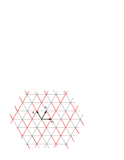
Figure 6: An illustration of the triangular lattice and the mean field ansatz Eq.(18). The pairing term is positive on the red bonds and negative on the black bonds.Sorella

This state is first studied in Ref.Sorella . When $\mu\rightarrow-\infty$, the Gutzwiller projected RVB state derived from the above ansatz evolves into the short range RVB state proposed by Anderson on triangular latticeAnderson . On the other hand, when $\mu=0$, it becomes a rather good variational ground state of the Heisenberg model on triangular lattice and possesses Dirac type spinon excitation at low energy. The RVB state for general value of $\mu$ can be viewed as an interpolation between these two limits.

For nonzero value of $\mu$, the gauge symmetry of the ansatz is broken to $Z_{2}$ and the spin excitation is fully gapped. At the same time, the RVB amplitude is short ranged and the sign of the wave function is frustrated. So we have every reason to expect a robust $Z_{2}$ topological order in this state.

Figure 7: The contribution from the sign and amplitude of the wave function to the Renyi entanglement entropy in the state RVB-II. The subsystem is now a $L\times L$ rhombic region on the triangular lattice and the total system size is fixed at $20\times 20$.

Figure 8: The TEE of the state RVB-II as a function of the subsystem size. Here $L_{A}$ is the linear scale of a rhombic region on triangular lattice. The total system size is fixed at $20\times 20$.

In the calculation we set $\mu=-30$ to produce a rather short ranged RVB amplitude. Unlike the state RVB-I, the state RVB-II has a fully frustrated sign. We find the contribution from the sign now makes up a much larger portion in the total entanglement entropy. This is illustrated in Fig.7. The result for TEE is shown in Fig.8. The TEE is seen to converge steadily to the expected value of $\ln 2$ for a spin liquid with $Z_{2}$ topological order.

In a previous studyVishwanath1 , it is found that in a critical RVB state the logarithmic correction to the area law is mainly contributed by the sign of the wave function. To see how the sign of the wave function would contribute to TEE, we have plotted in Fig.9 the contribution to TEE from the sign and the amplitude of the wave function separately. A key observation is that for both the state RVB-I and RVB-II, the contribution from the sign and that from the amplitude always have opposite signs. It is always the sign, rather than the amplitude of wave function that generate a positive contribute to TEE. It is also interesting to note that although $S_{2}^{\mathrm{amp}}>S_{2}^{\mathrm{sign}}$ in both RVB-I and RVB-II, it is the contribution from the sign that dominate the TEE. This indicate that the topological property of the RVB state is mainly determined by its sign structure.

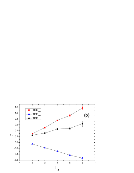
Figure 9: The contribution of the sign and the amplitude of the wave function to the TEE in the state RVB-I(a) and RVB-II(b). The total system size is fixed at $16\times 16$ and in (a) and is fixed at $20\times 20$ in (b).

VI VI. Discussions

In this paper, we have evaluated the TEE for two Gutzwiller projected Fermionic RVB states. Both states are derived from mean field ansatz with a $Z_{2}$ gauge structure and a full gap to spin excitations. Following effective field theory arguments, both states should exhibit $Z_{2}$ topological order. However, from the result of TEE we find the two states have different topological properties. With new tricks to improve the convergence of TEE, we are able to show that the spin liquid state RVB-I studied in Ref.Vishwanath does not support $Z_{2}$ topological order, while the spin liquid state RVB-II proposed in Ref.Sorella exhibits robust $Z_{2}$ topological order.

These results indicate that something beyond the effective field theory is important to the topological property of a RVB state. We find both a long ranged RVB amplitude and an unfrustrated sign in the RVB wave function can act to suppress the vison gap and thus the topological order in a RVB state. It is important to note that for the Fermionic RVB state, the RVB amplitude need not be short ranged even if the system has a large spin gap and that its spin correlation is extremely short ranged. The gap node deep inside the Fermi surface can have profound effect on the long wavelength behavior of the system. This is markedly different from a Bosonic RVB state, for which a full spin gap always corresponds to a short ranged RVB amplitude.

We have also tested topological degeneracy on the state RVB-I. We find the result implies a very small or even zero vison gap for the state RVB-I, which is consistent with the conclusion we get from the result of TEE. To our knowledge, this is for the first time that the topological property of a RVB state is studied from both the TEE and the topological degeneracy perspective with consistent conclusions reached. We also find that it is the sign, rather than the amplitude of the wave function that dominates the TEE and is responsible for a positive value of TEE in the Gutzwiller projected RVB state. Since a positive TEE is the signature of nonlocal entanglement in the system, we find the nonlocal entanglement in a RVB state is mainly encoded in its sign structure. This is consistent with previous studies in which it is found that a Marshall sign rule is at the origin for the absence of topological order in certain spin liquidsLi1 ; Li2 ; Sorella1 .

From the effective field theory point of view, a $Z_{2}$ gauge structure and a fully gapped spin excitation spectrum is enough to guarantee the stability of the saddle point against gauge fluctuation up to Gaussian level. Since Gutzwiller projection just amounts to gauge averaging on the saddle point, we expect the Gutzwiller projected RVB state to have the same topological property as the saddle point action of effective field theory, if the fluctuation effect beyond the Gaussian level can be neglected in the long wavelength limit. Our results show that this is not always true. Thus, certain singular fluctuation mode beyond the Gaussian level is important for the topological property of RVB state. It is an interesting problem to study how such singular gauge mode are related to the emergence of the Marshall sign rule structure of the Gutzwiller projected wave function and to the long ranged nature of the RVB amplitude.

In conclusion, from our results it is clear that the effective field theory at the Gaussian level misses two pieces of information that is important for the topological property of a RVB state. The first one is the sign structure of the Gutzwiller projected wave function. The second one is the range of the RVB amplitude of the RVB state. The effective field theory can predict the topological property of a RVB state reliably only when both of these information are accounted for.

This work is supported by NSFC Grant No. 10774187, No. 11034012 and National Basic Research Program of China No. 2010CB923004.

References

- (1) Introduction to Frustrated Magnetism, Materials, Experiments, Theory, C. Lacroix, P. Mendels and F. Mila eds., Springer, (2010).
- (2) A. Kitaev and J. Preskill, Phys. Rev. Lett., 96 110404, (2006).
- (3) M. Levin and X.-G. Wen, Phys. Rev. Lett., 96 110405, (2006).
- (4) P. A. Lee, N. Nagaosa and X. G. Wen Rev. Mod. Phys. 78, 17 (2006).
- (5) S. Yunoki and S. Sorella, Phys. Rev. B 74, 014408 (2006).
- (6) Tao Li and Hong-Yu Yang, Phys. Rev. B, 75, 172502(2007).
- (7) Tao Li, EPL, 93 37007 (2011).
- (8) Tao Li, arXiv:1101.1352.
- (9) S. Sorella, Y. Otsuka and S. Yunoki, arXiv:1207.1783 and Scientific Report, in press (2012).
- (10) D. A. Ivanov and T. Senthil, Phys. Rev. B 66, 115111 (2002).
- (11) A. Paramekanti, M. Randeria, and N. Trivedi, Phys. Rev. B 71, 094421 (2005).
- (12) S. Furukawa and G. Misguich, Phys. Rev. B, 75, 214407, (2007).
- (13) H. C. Jiang, Z. Wang, L. Balents, Nature Physics 8, 902 (2012).
- (14) Y. Zhang, T. Grover, and A. Vishwanath, Phys. Rev. B 84, 075128 (2011).
- (15) Y. Zhang, T. Grover, and A. Vishwanath, Phys. Rev. B 85, 199905(E) (2012) .
- (16) Y. Zhang, T. Grover, and A. Vishwanath, Phys. Rev. Lett. 107, 067202 (2011).
- (17) P. W. Anderson, Mater. Res. Bull. 8 2 153, (1973).
- (18) S. T. Flammia, A. Hamma, T. L. Hughes, and X.-G.Wen, Phys. Rev. Lett., 103, 261601, (2009).
- (19) M.B. Hastings, I. Gonzalez, A.B. Kallin, and R.G. Melko, Phys. Rev. Lett., 104 157201, (2010).
- (20) T. Li and F. Yang, Phys. Rev. B 81, 214509 (2010).
- (21) Jiquan Pei, Qiang Han, Haijun Liao and Tao Li, arXiv:1211.1504.
- (22) L. Capriotti, F. Becca, A. Parola, and S. Sorella, Phys. Rev. Lett. 87, 097201 (2001).
- (23) D.S. Rokhsar and S.A. Kivelson, Phys. Rev. Lett., 61 2376, (1988).
- (24) N. Read and D. Green, Phys. Rev. B 61 10267, (2000).