Abstract

The MC toy model for Bose-Einstein correlations (BEC) is considered to make a best choice from different reference distributions. It occurs that the minimal bias in the BEC parameters estimation is provided by the reference sample which is being simulated from ”observed” sample by the turn of all $\vec{p_{t}}$ vectors in an event by a random $\delta\phi$.

It proposed to use similar approach in the analysis $C_{2}(\Delta\eta,\Delta\phi$) correlation. To make the analysis less dependent on reference sample, new definition of $\Delta\phi$ is implemented as the angle between vectors $p_{1}$ and $p_{2}$ in the transverse plane. Then $C_{1}(\Delta\phi)$ correlation can be studied without a reference sample subtraction.

The ridge in $C_{2}(\Delta\eta,\Delta\phi$) correlation appears if an appropriate cut in Q-value ($Q=p_{2}-p_{1}$) is applied.

1 Introduction

One of the way to study the space-time picture of hadronic interaction is to measure the correlations between two identical particles which momenta are close to each other. This correlations are used to estimate the size of the domain, from which particles produced are emitted.

Consider the amplitude $M(r_{1},r_{2})$ in coordinate representation in which two identical pions, $\pi_{1}$ and $\pi_{2}$, are emitted at the points $r_{1}$ and $r_{2}$ correspondingly. The coordinates $r_{1}$, $r_{2}$ can not be measured, and instead one does estimate pions momenta quantities $p_{1}$ and $p_{2}$ . So we have to take the Fourier transform

$$M_{a}(p_{1},p_{2})=\int\frac{d^{4}r_{1}}{(2\pi)^{4}}e^{ip_{1}r_{1}}\frac{d^{4}r_{1}}{(2\pi)^{4}}e^{ip_{2}r_{2}}M(r_{1},r_{2}).$$ (1)

Besides this we have to consider the permutation of two identical pions. That is we have to add to $M_{a}$ the amplitude

$$M_{b}(p_{1},p_{2})=\int\frac{d^{4}r_{1}}{(2\pi)^{4}}e^{ip_{2}r_{1}}\frac{d^{4}r_{1}}{(2\pi)^{4}}e^{ip_{1}r_{2}}M(r_{1},r_{2}),$$ (2)

where the pion with momentum $p_{2}$ was emitted from the point $r_{1}$ and wise versa. This can be written as

$$M(p_{1},p_{2})=M_{a}+M_{b}=M_{a}\cdot(1+e^{irQ}),$$ (3)

where the 4-vectors $r=r_{1}-r_{2}$ and $Q=p_{2}-p_{1}$ .

Finally the cross section takes the form

$$\frac{E_{1}E_{2}d^{2}\sigma}{d^{3}p_{1}d^{3}p_{2}}=\frac{1}{2!}|M_{a}|^{2}<2+2e^{irQ}>=|M_{a}|^{2}(1+<e^{irQ}>).$$ (4)

Here the factor $1/2!$ reflects the identity of two pions and the angular brackets indicates the averaging over the ($r_{1},r_{2}$) space distribution. Assuming, for simplicity, the Gaussian form we get $<e^{irQ}>=e^{-<r^{2}>Q^{2}}$.

Thus the width of a peak at small momenta difference $Q\to 0$ characterizes the size $<r>$ of the domain from which the pions were emitted.

The general definition of a correlation function of 2 variables - $p_{1}$ and $p_{2}$ can be written as

$$C_{2}(p_{1},p_{2})=\frac{P(p_{1},p_{2})}{P_{ref}(p_{1},p_{2})}.$$ (5)

The value $P_{ref}(p_{1},p_{2})$ is called a reference function, artificial function with switched off the correlation under search . Usual task is to extract correlation $C_{2}$ from the ”measured” value $P(p_{1},p_{2})$. In the following we will consider Bose-Einstein correlations (BEC) in the multi-particle final state (MPS) in pp-collisions. Suppose that BEC correlation is determined by $P(p_{1},p_{2})$ with the reference $P_{ref}(p_{1},p_{2})$. Usually MC generators simulate MPS without BEC. In the following the ATLAS MC [1] of the pp-interaction with 7 TeV center of mass energy is used. In the MC event sample there is no BE correlations , but known hadronic resonance states are ”produced”.

The distributions of identical bosons should be influenced by $BEC$. The proximity in phase space between final state particles with 4-momenta $p_{1}$ and $p_{2}$ can be quantified by

$$Q=\sqrt{-(p_{1}-p_{2})^{2}}.$$ (6)

The BEC effect is observed as an enhancement at low $Q\sim 300MeV$. To extract the effect one can compare measured Q-spectra with similar one but without BEC, with reference spectra . Then the ratio

$$R(Q)=\frac{\frac{dN}{dQ}-\frac{dN_{ref}}{dQ}}{\frac{dN_{ref}}{dQ}}$$ (7)

can be fitted with an appropriate formulae

$$R(Q)=F(rQ)+a+bQ$$ (8)

F(rQ) is the Fourier transform of the spatial distribution of the emission region with an effective size $\langle r\rangle$. The function can be parameterize as a linear exponent $F=Ce^{-r_{e}Q}$ or a Gaussian $F=Ce^{-r_{g}^{2}Q^{2}}$. The parameter $b$ may be accounted for a long range correlation.For the same $\langle r\rangle$ there is quite simple relation between these two cases :

$$r_{e}=\sqrt{\pi}r_{g}.$$ (9)

These two choices are connected to different radiation sources distribution inside the emission region. The exponential form approximates the case when radiation is originated from the surface of the sphere with radius $r_{e}$. The second form describes the radiation in space $\sim e^{-r_{g}^{2}Q^{2}}$. The fit of the same distribution $\frac{dN_{ss}}{dQ}$ with these two cases gives r-parameter ratio as in ( 9). The exponential fit is a bit better and will be used in the following.

2 MC BEC model and different reference functions

Two values of $\frac{dN}{dQ}$ are measured in the experiment: $\frac{dN_{ss}}{dQ}$ for the like sign particle pairs and $\frac{dN_{us}}{dQ}$ for the unlike sign case. To simulate BEC into MC distribution , each entry into $\frac{dN_{ss}}{dQ}$ can be weighted by the function

$$W(Q)=1.+e^{-rQ}$$ (10)

to produce $\frac{dN_{mod}}{dQ}$. The value $r$ is fixed equal to 2fm. Of course, such model is the oversimplified toy but good enough to illustrate difference between reference functions.

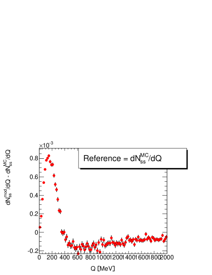
(a) The difference of normalized distributions $\frac{dN_{mod}}{dQ}-\frac{dN{{}_{ss}}^{ref}}{dQ}$

(b) Fit of the ratio $R(Q)=\frac{\frac{dN_{mod}}{dQ}-\frac{dN{{}_{ss}}^{ref}}{dQ}}{\frac{dN{{}_{ss}}^{ref}}{dQ}}$

Figure 1: MC Model fit with the ”ideal” reference

First consider the ideal case when MC $\frac{dN_{ss}}{dQ}$ will be used as the reference function $\frac{dN^{ref}_{ss}}{dQ}$. Fig  1 shows the difference $\frac{dN_{mod}}{dQ}-\frac{dN^{ref}_{ss}}{dQ}$ and the result of the fit of the ratio (7) with the formulae (8) . The result is somewhat trivial and can be considered as a ”goodness” of the MC generator. The procedure used might be looked as switching ON the BEC correlation, to add such correlation to MC procedure.

In the BEC analyses of experimental data different approaches have been explored and it is worth to compare known reference functions with the use of the toy MC model.

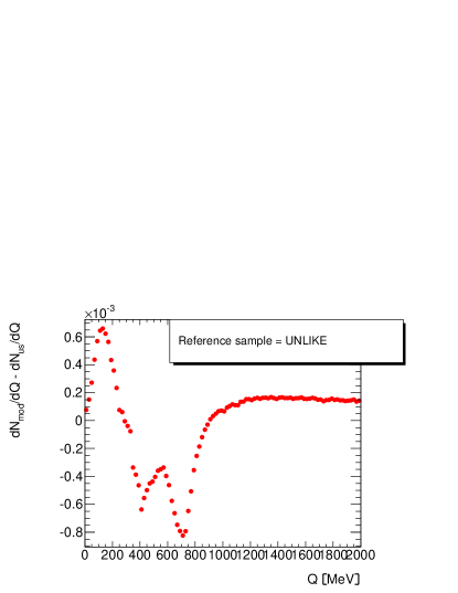
(a) The difference of normalized distributions ($\frac{dN_{mod}}{dQ}-\frac{dN_{us}}{dQ}$ )

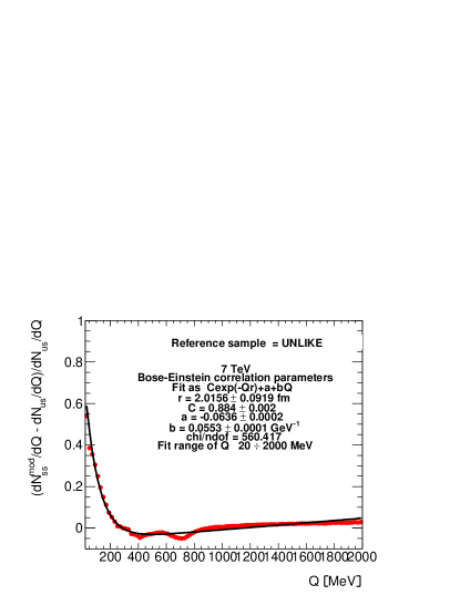
(b) Fit of the ratio $R(Q)=\frac{\frac{dN_{m}od}{dQ}-\frac{dN_{us}}{dQ}}{\frac{dN_{u}s}{dQ}}$

Figure 2: MC Model fit with the $\frac{dN}{dQ}$ for unlike sign pairs as the reference

The unlike Q-distribution looks as a natural choice because there should be no BEC for the unlike sign pairs. The source radius from the fit is close to the model value ( Fig  2), however the resonances contribution makes fit quality bad. The contributions of the $\rho^{0}$ and the remnants of $\eta$ mesons are clearly seen.

One has to find a way to switch OFF BEC from the ”observed” $\frac{dN_{mod}}{dQ}$ distributions. It looks as an easiest way to construct the $\frac{dN{{}_{ss}}^{ref}}{dQ}$ from two independently detected events: one momentum vector is taken from event under analysis, and the second - from a preceding events. The result is strongly dependent on requirements of such event selection. Moreover, such requirements formulation is rather arbitrary.

Another approach is to emulate independent event sample with the use of the events set under consideration. The ”referenced” event will have at least the same particle multiplicity,the same numbers of positive and negative charged particles. Evidently, such procedure will work as a blind correlation terminator because there is no any BEC ”marker” on a particular entry. The hope can be that pairs with small Q-values will be replaced by pairs which had higher Q-value before the transformation. The reference distribution $\frac{dN{{}_{ss}}^{ref}}{dQ}$ will contain one vector from the real event and another from the reference one.

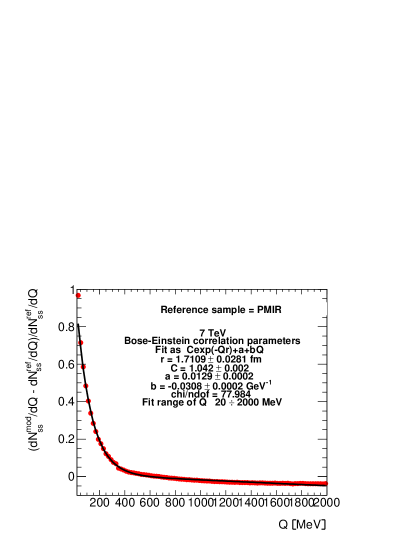
(b) Fit of the ratio $R(Q)=\frac{\frac{dN_{m}od}{dQ}-\frac{dN{{}_{ss}}^{ref}}{dQ}}{\frac{dN{{}_{ss}}^{ref}}{dQ}}$

Figure 3: MC Model fit of the ratio $R(Q)$ where the reference sample consists of real events with all 3-vector momentum reflected in space

The standard procedure to prepare mirror sample from the original one is to change in the event all momenta 3-vectors as $\vec{p}\rightarrow-\vec{p}$ (PMIR case). It would be good if events (and the detector) have such symmetry. The reference sample is the result of measurements with the detector identical to the real one but in the mirror space. Fig  3 illustrate results of such procedure. We do see that the distribution $\frac{dN{{}_{ss}}^{ref}}{dQ}$ is different from the model too much. In particular there is no entries in the reference distribution if Q-value in the real events is smaller than $\sim 300MeV$ : the procedure removes all small Q entries from the reference Q-distribution, not only BEC entries. In other words, the BEC contribution will be overestimated and the ratio (8) Q-distribution will be wider ( compared with Fig  1) and the $r$-parameter of (8) will be smaller than in the model.

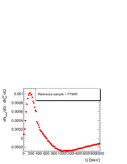
(a) The difference of normalized distributions $\frac{dN_{mod}}{dQ}-\frac{dN{{}_{ss}}^{ref}}{dQ}$

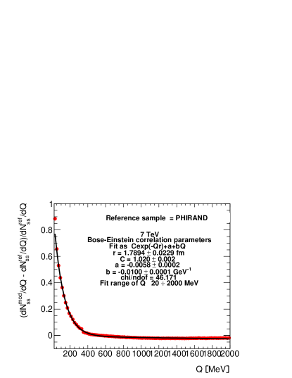
(b) Fit of the ratio $R(Q)=\frac{\frac{dN_{m}od}{dQ}-\frac{dN{{}_{ss}}^{ref}}{dQ}}{\frac{dN{{}_{ss}}^{ref}}{dQ}}$

Figure 4: MC Model fit of the ratio $R(Q)$ where the reference sample consists of real events with all $\vec{p}_{t}$ momentum reflected in the transverse plane

The better way might be if the reflection is made only in the transverse plane $\vec{p}_{t}\rightarrow-\vec{p}_{t}$ (PTMIR case). The results are a bit closer to the model values but still there is no small Q events in the reference distribution if the model Q-values is smaller than $\sim 300MeV$ ( Fig 4).

One gets a bit better reference distribution if vectors $\vec{p}_{t}$ in an observed event will be turned by a random value of $\delta\phi$ : the same turn for all tracks - PHIRAND case , or each track is turned by a random angle - PHIWIDE case ( Fig  6). Fit parameters for the PHIWIDE case is found to be closer to the model than in all previous cases.

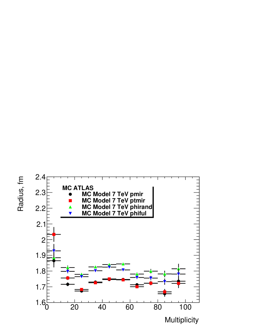
Figure 7: Fit results for different reference samples

The model we consider, the radiation zone radius has a constant value. However one might suspect that ”imperfection” of reference samples is larger at small particles multiplicity. This is the case indeed ( Fig  7). The samples with the reflection algorithms produce quite detectable multiplicity dependence. The approach with the random $\vec{p}_{t}$ turn again looks better.

Another important feature is the value of a systematic uncertainty. One can produce the reference sample of MC events without BEC and estimate a value of the source radius with different reference samples. It occurs that the value is quite small ( .15 fm, Fig  LABEL:fig:mc_fit_no_BEC) and might be consider as a contribution of non-BE correlation with small Q value or as a systematic uncertainty. In the following, we will see that non-BE correlation at small Q exists indeed.

3 2- and 3-dimensional correlations

Until now, we have used 1-dimensional distribution - number of events as a function of Lorentz invariant value Q. This is a natural approach for a simple fit to measure phenomenon parameters . Another way have to be considered in the case of a search of deviations from a phase space prediction with a smooth reaction amplitude. Usually 2-dimensional correlations is being used. Let us consider the traditional correlation plot for like sign pairs where differences

$$\begin{split}\Delta\phi_{2\pi}=\phi_{2}-\phi_{1},\\ \Delta\eta=\eta_{2}-\eta_{1}\end{split}$$ (11)

will be taken as arguments - $C_{2}(\Delta\phi_{2\pi},\Delta\eta)$. Q-value and $N_{ch}$ ( number of charged particles in the event) can be used as additional arguments to form 3-dimensional correlations $C_{3}(\Delta\phi_{2\pi},\Delta\eta,Q)$ and $C_{3}(\Delta\phi_{2\pi},\Delta\eta,N_{ch})$.

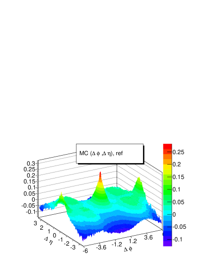
(b) MC $R(\Delta\phi,\Delta\eta)$ =$\frac{C_{2}(\Delta\phi,\Delta\eta)-C_{2}^{ref}(\Delta\phi,\Delta\eta)}{C_{2}^{ref}(\Delta\phi,\Delta\eta)}$

Figure 8: MC $C_{2}(\Delta\phi,\Delta\eta$) for like sign pairs correlation, $\Delta\phi=\Delta\phi_{2\pi}$

Fig  8 shows several correlation plots. If particles would have the uniform distribution for $\eta(-2.5,2.5)$ and for $\phi(-\pi,\pi)$ , then the values $C_{1}(\Delta\eta)$ and $C_{1}(\Delta\phi_{2\pi})$ will have triangle distribution in the range $\eta(-5.,5.)$ and $\phi(-2\pi,2\pi)$. For these reasons $C_{2}(\Delta\phi_{2\pi},\Delta\eta)$ looks as a pyramid. Except rather strong correlation at $\Delta\phi_{2\pi}\approx\Delta\eta\approx 0$ nothing significant can be seen . One have to subtract a reference distribution (one of the $p_{t}$ vector of the pair is turned by a random $\delta\phi$ ) to see some additional structure. Unfortunately small nonuniformity might appear artificially because of imperfections of the reference sample.Some features are connected with definition of $\Delta\phi_{2\pi}$: evidently,$\Delta\phi_{2\pi}=\pm 2\pi$ is the same as $\Delta\phi_{2\pi}=0.$

It is better to change the definition of $\Delta\phi$ :

$$\begin{split}\Delta\phi_{\pi}=\phi_{2}-\phi_{1},|\phi_{2}-\phi_{1}|<\pi\\ \Delta\phi_{\pi}=\phi_{1}-\phi_{2},|\phi_{2}-\phi_{1}|>\pi\end{split}$$ (12)

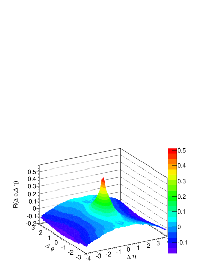
(b) MC $R(\Delta\phi,\Delta\eta)$ =$\frac{C_{2}(\Delta\phi,\Delta\eta)-C_{2}^{ref}(\Delta\phi,\Delta\eta)}{C_{2}^{ref}(\Delta\phi,\Delta\eta)}$ for unlike sign pairs

Figure 9: MC $C_{2}(\Delta\phi,\Delta\eta$) ,$\Delta\phi=\Delta\phi_{\pi}$

$\Delta\phi_{\pi}$ will have a uniform distribution in the range ($-\pi,\pi$) in the absence of correlations and to study correlations one has no need for any reference to subtract. Fig  9 shows $C_{2}(\Delta\phi,\Delta\eta)$ before and after reference subtraction. Similar plot for unlike sign pairs is shown also . Strong correlation is independent on charge of particles.

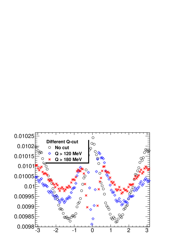
Figure 11: MC $C_{1}(\Delta\phi$) distribution with different cuts in Q value

Let us consider other correlations $C_{2}(\Delta\phi,Q)$ and $C_{2}(\Delta\eta,Q)$ (Fig  10). An enhancement at small Q value can be expected. Q is small if $\Delta\phi\sim 0$ and $\Delta\eta\sim 0$ ( momentum value of particles in pairs are larger than masses) ,independent on the momentum values and the charges of particles. At the same time at large Q value there is a dip at $\Delta\phi\sim 0$ and ( $\Delta\eta\sim 0$ ). Then after integration in Q , there might be full compensation of the enhancement at small Q , if there is no dynamical reason to make an enforcement of this enhancement. By other words, with an appropriate cut in Q value, small $\Delta\phi$ and $\Delta\eta$ correlation can be suppressed (Fig  11). An effect of dynamical correlations exists only when Q is less than $\sim 200MeV$. After such cut nonuniformity in $\Delta\phi$ decreases from $\sim 4\%$ to $\sim 1\%$. Very important that such behavior is the same for like sign and unlike sign pairs ( except natural traces of resonances at $Q>400$ MeV) .

The next step is to have a look an influence of such Q cuts on 2-dimensional plots (Fig  12). The ”Long-Range, Near-Side Correlations” (ridge) starts to be appear. Such effect has not been seen in MC before ( see [3])not only because Q-cut never was used before, but also because of different way to construct the reference sample ( see in the follows). The ridge was observed [3] in the data analysis of pp-collisions at the LHC at 7TeV in high multiplicity events with selection of pairs of charged particles with $p_{t}$ in the range (1-3) GeV. In MC distribution there is no trace of a ridge, if only small $p_{t}$ cut has been done. Fig  13 shows the correlations for particles with $p_{t}>1GeV$. The multiplicity cut only decrease statistics but does not change the conclusion. By other words, the selection of pairs of particles with $Q>200$ MeV can be good tool for search of a ridge effect.

4 Conclusions

Rather simple MC model for Bose-Einstein Correlations is used to judge the quality of different ways to extract the BEC from observable distribution. Several emulated reference samples have been considered. The reference sample with random turn of observed transverse momentum vector $\vec{p}_{t}$ ( $\phi$ randomization ) provides the fit results closest to the model values.

Such approach is implemented for the analysis of $C_{2}(\Delta\phi,\Delta\eta$) correlation. In the traditional definition of $\Delta\phi_{2\pi}$, to extract correlations the subtraction of a reference distribution is the must. New definition $\Delta\phi_{\pi}$ as the angle between $\vec{p}_{t1}$ and $\vec{p}_{t2}$ makes $\Delta\phi_{\pi}$ distribution uniform with small contribution from an intrinsic correlations. For this reason the $C_{1}(\Delta\phi_{\pi})$ can be studied without any reference. It is shown that at small Q-value there might be two kind of $C_{1}(\Delta\phi_{\pi})$ correlation - kinematical and dynamical. At large Q there is $C_{1}(\Delta\phi_{\pi})$ anticorrelation. Then so called short-range correlation ( $\Delta\phi_{\pi}\sim 0$ ) can be suppressed by an appropriate cut in the Q- value.

(a) The difference of normalized distributions $\frac{dN_{mod}}{dQ}-\frac{dN{{}_{ss}}^{ref}}{dQ}$

(a) The difference of normalized distributions $\frac{dN_{mod}}{dQ}-\frac{dN{{}_{ss}}^{ref}}{dQ}$

(b) Fit of the ratio $R(Q)=\frac{\frac{dN_{m}od}{dQ}-\frac{dN{{}_{ss}}^{ref}}{dQ}}{\frac{dN{{}_{ss}}^{ref}}{dQ}}$

Figure 5: MC Model fit of the ratio R(Q) where the reference sample consists of real events with all $\vec{p}_{t}$ momentum turned by the same random $\delta\phi$

(a) The difference of normalized distributions $\frac{dN_{mod}}{dQ}-\frac{dN{{}_{ss}}^{ref}}{dQ}$

(b) Fit of the ratio $R(Q)=\frac{\frac{dN_{m}od}{dQ}-\frac{dN{{}_{ss}}^{ref}}{dQ}}{\frac{dN{{}_{ss}}^{ref}}{dQ}}$

Figure 6: MC Model fit of the ratio R(Q) where the reference sample consists of real events with all $\vec{p}_{t}$ momentum turned by the same random $\delta\phi$

(a) MC $C_{2}(\Delta\phi,\Delta\eta)$ for like sign pairs correlation

(a) MC $R(\Delta\phi,\Delta\eta)$ =$\frac{C_{2}(\Delta\phi,\Delta\eta)-C_{2}^{ref}(\Delta\phi,\Delta\eta)}{C_{2}^{ref}(\Delta\phi,\Delta\eta)}$ for like sign pairs

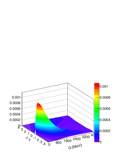
(a) MC $C_{2}(Q,\Delta\eta$) correlation

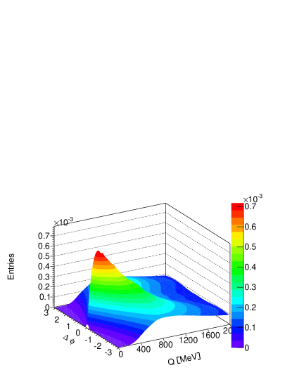
(b) MC $C_{2}(Q,\Delta\phi$) unlike sign correlation

Figure 10: MC $C_{2}(Q,\Delta\phi)$ and $C_{2}(Q,\Delta\eta$) correlations

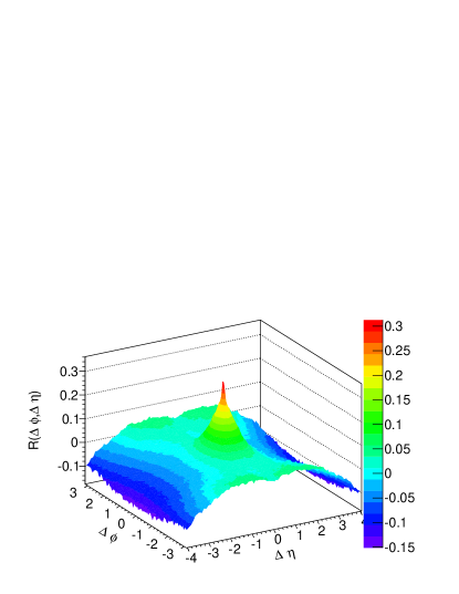
(a) MC $R(\Delta\phi,\Delta\eta)$ correlation without Q cut

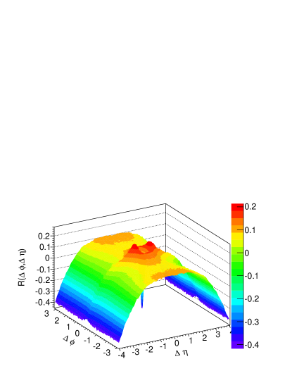
(b) MC $R(\Delta\phi,\Delta\eta)$ correlation with $Q>120$ MeV cut

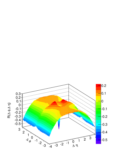
(c) MC $R(\Delta\phi,\Delta\eta)$ correlation with $Q>200$ MeV cut

Figure 12: MC $R(\Delta\phi,\Delta\eta)$ correlation

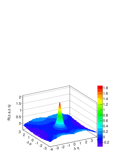
(a) MC $R(\Delta\phi,\Delta\eta)$ correlation without Q cut

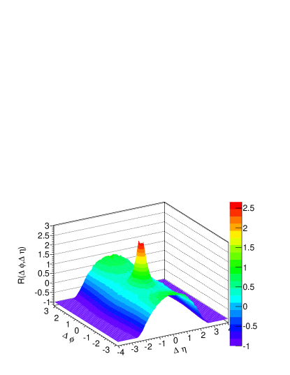
(b) MC $R(\Delta\phi,\Delta\eta)$ correlation with $Q>120$ MeV cut

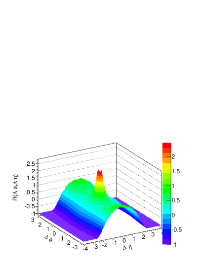
(c) MC $R(\Delta\phi,\Delta\eta)$ correlation with $Q>200$ MeV cut

Figure 13: MC $R(\Delta\phi,\Delta\eta)$ correlation for pairs with $p_{t}^{min}=1GeV$

References

- [1] ATLAS Collaboration, ATLAS Monte Carlo Tunes for MC09, ATL-PHYS-PUB-2010-002.
- [2] Charged particle multiplicities in pp interactions measured with the ATLAS detector at the LHC,New J.Phys. 13(2011) 053033
- [3] Observation of Long-Range Near-Side angular correlations in proton-proton collisions at the LHC, JHEP 1009:091, 2010.