Feshbach Resonance in a Synthetic Non-Abelian Gauge Field

Abstract

We study the Feshbach resonance of spin-$1/2$ particles in the presence of a uniform synthetic non-Abelian gauge field that produces spin orbit coupling along with constant spin potentials. We develop a renormalizable quantum field theory that includes the closed channel boson which engenders the Feshbach resonance, in the presence of the gauge field. By a study of the scattering of two particles in the presence of the gauge field, we show that the Feshbach magnetic field, where the apparent low energy scattering length diverges, depends on the conserved centre of mass momentum of the two particles. For high symmetry gauge fields, such as the one which produces an isotropic Rashba spin orbit coupling, we show that the system supports two bound states over a regime of magnetic fields for a negative background scattering length and resonance width comparable to the energy scale of the spin orbit coupling. We discuss the consequences of these findings for the many body setting, and point out that a broad resonance (width larger than spin orbit coupling energy scale) is most favourable for the realization of the rashbon condensate.

Simulation of quantum matter using cold atomsKetterle and Zwierlein (2008); Bloch et al. (2008); Esslinger (2010); Cirac and Zoller (2012) has emerged as a very active area of physics research. This owes to the unprecedented tunability that cold atom systems offer in terms of creating hamiltonians with desired one particle levels and interactions. With the recent advances in synthetic gauge fieldsLin et al. (2009a, b, 2011); Wang et al. (2012); Cheuk et al. (2012) the possibility of using cold atoms to simulate even exotic topological states has been significantly enhanced.

These advances have motivated many an effort in the theoretical study of bosonsStanescu et al. (2008); Wang et al. (2010); Ho and Zhang (2011); Cong-Jun et al. (2011) and fermionsVyasanakere and Shenoy (2011); Vyasanakere et al. (2011); Yu and Zhai (2011); Hu et al. (2011); Gong et al. (2011); Iskin and Subaş ı (2011); Han and Sá de Melo (2012); Vyasanakere and Shenoy (2012); Cui (2012); Zhang et al. (2012); Goldman et al. (2012) in synthetic gauge fields. Uniform non-Abelian SU(2) gauge fields induce a Rashba-like spin orbit coupling. For fermions interacting with a contact singlet attraction described by an energy independent scattering length $a_{s}$, a non-Abelian gauge field “amplifies the attractive interaction”Vyasanakere and Shenoy (2011) rendering the critical scattering length required for bound state formation negative. Indeed high symmetry non-Abelian gauge fields induce a bound stateVyasanakere and Shenoy (2011) for any scattering length(see also, Cui (2012); Zhang et al. (2012)). For a finite density of fermions, increasing the strength of the spin-orbit coupling $(\lambda)$ induces a crossover from a BCS state comprising of large pairs to a BEC of a new kind of boson, the rashbon, even when the scattering length $a_{s}$ is small and negative. The rashbon is the two fermion bound state obtained with infinite scattering length, and is realized for large $\lambda$ even when $a_{s}$ is small and negative. In other words, the requirement for the realization of the rashbon is that $|\lambda a_{s}|$ is large. Since $\lambda$ is determined by the lasers used to produce the spin-orbit couplingDalibard et al. (2011), one may use a Feshbach resonance to tune the scattering length be in this desired regime. These considerations, inter alia, provide the natural motivation for this study.

A Feshbach resonanceTimmermans et al. (1999); Chin et al. (2010) is obtained when the bound state of the closed (“triplet”) channel whose energy is determined by the magnetic field $B$, crosses the scattering threshold of the open (“singlet”) channel. The two channels are coupled by the hyperfine interaction and this produces enhanced scattering of the two particles in the open channel resulting in a magnetic field dependent scattering lengthMoerdijk et al. (1995)

$$a_{0}(B)={a}_{bg}\left(1-\frac{W}{B-B_{\infty}}\right),$$ (1)

where ${a}_{bg}$ is the background scattering length of the open channel, $B_{\infty}$ is the field (Feshbach field) which produces a resonant scattering length, and $W$ is the width of the resonance. While $a_{0}(B)$ pertains to particles at the scattering threshold, scattering at finite energies can be strongly energy dependent for narrow resonancesChin et al. (2010), and can have interesting effects in many body systems.Kokkelmans et al. (2002); Ho et al. (2012)

In this paper, we develop a renormalizable quantum field theory of the Feshbach resonance in the presence of a synthetic gauge field. We obtain explicit expressions for the fermion scattering $T$-matrix for a generic gauge field. An important point uncovered by this analysis is that the gauge field renders the Feshbach field $B_{\infty}$ momentum dependent, i. e., $B_{\infty}$ depends on the centre of mass momentum of the two particles. Further, for high symmetry gauge fields, we show that in a regime of magnetic field, there are two accessible bound states when the background scattering length is negative and the width is comparable to the spin orbit coupling scale. We discuss the consequences of these results in the many body setting and the conditions that will enable the experimental realization of the rashbon condensate.

Quantum Field Theory: Consider a quantum field $\Psi_{n}(x)$ ($x=(\tau,\bm{r})$, $\tau$ is imaginary time, $\bm{r}$ is position vector in 3D) where the subscript $n=1,...,M(M\geq 3)$ denotes the hyperfine label of the atom (fermions in this paper). Of particular interest are the hyperfine labels $n=1,2$, which serve as the two spin species of interest. The $1$-$2$ interaction in the open (singlet) channel is described by a contact potential $\upsilon$. The closed (triplet) channel has a bound state described by a bosonic field $\phi(x)$ called the closed channel boson (CCB). The CCB, whose energy is $\varepsilon_{\phi}(B)=B+B_{a}$ ($B$ is the magnetic field, and $B_{a}$ is an “adjustment field”, see below), couples to the singlet density $S(x)$ of the open channel via hyperfine coupling $\upkappa$. The position dependent laser coupling of the hyperfine states that produces the gauge field is denoted by $H^{L}_{nn^{\prime}}(\bm{r})$. At an inverse temperature $\upbeta$, this scenario is described by the action ($\int\mbox{d}{x}=\int_{0}^{\upbeta}\mbox{d}{\tau}\int_{\Omega}\mbox{d}{\bm{r}}$, $\Omega$ is the volume, repeated indices summed)

$$\begin{split}&{\cal S}[\Psi,\phi]=\int\mbox{d}{x}\Psi^{\star}_{n}(x)\left(\delta_{n,n^{\prime}}\left(\frac{\partial}{\partial\tau}-\frac{\mbox{\boldmath$\nabla$}^{2}}{2}\right)+H_{nn^{\prime}}^{L}(\bm{r})\right)\Psi_{n}(x)\\ &+\frac{\upsilon}{2}\int\mbox{d}{x}S^{*}(x)S(x)+\frac{\upkappa}{\sqrt{2}}\int\mbox{d}{x}\left(\phi^{*}(x)S(x)+S^{*}(x)\phi(x)\right)\\ &+\int\mbox{d}{x}\phi^{*}(x)\left(\frac{\partial}{\partial\tau}-\frac{\mbox{\boldmath$\nabla$}^{2}}{4}+\varepsilon_{\phi}(B)\right)\phi(x).\end{split}$$ (2)

In the absence of the laser field this reduces to the well known two channel model.Timmermans et al. (2001); Duine and Stoof (2004); Braaten et al. (2008) Progress is made by “locally diagonalizing” $H_{nn^{\prime}}^{L}(\bm{r})$, and integrating out all but the lowest two states which are mostly of 1-2 character (see, for example, Liu et al. (2009)). These two new states are represented by the quantum fields $\psi_{\sigma}(x)$ where $\sigma=\uparrow,\downarrow$. The old 1-2 fields are related to the new ones via $\Psi_{n}(x)=U_{n\sigma}(\bm{r})\psi_{\sigma}(x)$, where $U_{n\sigma}(\bm{r}),n=1,2$ is a position dependent SU(2) matrix. Writing the action in terms of the new “spin-$\frac{1}{2}$” fields results in

$$\begin{split}&{\cal S}[\psi,\phi]=\int\mbox{d}{x}\psi^{\star}_{\sigma}(x)\left(\delta_{\sigma,\sigma^{\prime}}\frac{\partial}{\partial\tau}+H_{\sigma\sigma^{\prime}}(-i\mbox{\boldmath$\nabla$},{\bm{\lambda}})\right)\psi_{\sigma}(x)\\ &+\frac{\upsilon}{2}\int\mbox{d}{x}S^{*}(x)S(x)+\frac{\upkappa}{\sqrt{2}}\int\mbox{d}{x}\left(\phi^{*}(x)S(x)+S^{*}(x)\phi(x)\right)\\ &+\int\mbox{d}{x}\phi^{*}(x)\left(\frac{\partial}{\partial\tau}-\frac{\mbox{\boldmath$\nabla$}^{2}}{4}+\varepsilon_{\phi}(B)+\varepsilon_{sft}\right)\phi(x).\end{split}$$ (3)

Two points are to be noted. First, the $S(x)$ written in terms of $\sigma$ states is unchanged from the original. Second, we have considered the case where the CCB is a deep bound state of the closed channel potential and hence its wavefunction and kinetic energy are unaffected by the laser potential apart from a shift $\varepsilon_{sft}$. Taken together, this leaves $\upkappa$ unchanged. The term $H_{\sigma\sigma^{\prime}}(-i\mbox{\boldmath$\nabla$},{\bm{\lambda}})$ acting in the open channel now contains the uniform gauge filed (connection induced by $U_{n\sigma}(\bm{r})$, Moody et al. (1989)) and any other spin potential such as the detuning and Zeeman fieldsLiu et al. (2009), all of which are collectively described by ${\bm{\lambda}}$. In the following we set $\varepsilon_{sft}=0$. Eqn. (3) is the quantum field theory that describes the Feshbach resonance in the presence of the gauge field. Note that $\upsilon,\upkappa$ and $B_{a}$ are the bare coupling constants; the theory requires renormalization. This is accomplished by considering the two body problem.

Two body problem: The one particle eigenstates of $H_{\sigma\sigma^{\prime}}(-i\mbox{\boldmath$\nabla$},{\bm{\lambda}})$ are generalized helicity states $|\bm{k},\alpha\rangle=|\bm{k}\rangle\otimes|\chi_{\alpha}(\bm{k})\rangle$ with dispersion $\varepsilon_{\alpha}(\bm{k})$. Here $|\bm{k}\rangle$ is the momentum eigenstate, and $|\chi_{\alpha}(\bm{k})\rangle$ is a momentum dependent spin state determined by ${\bm{\lambda}}$ where $\alpha=\pm 1$ is the generalized helicity. Since the action (eqn. (3)) conserves momentum, we can construct two particle states of total momentum $\bm{q}$. The two particle state $|\bm{q},\bm{k},\alpha\beta\rangle=|\frac{\bm{q}}{2}+\bm{k},\alpha\rangle\otimes|\frac{\bm{q}}{2}-\bm{k},\beta\rangle$ has energy $\varepsilon_{\alpha\beta}(\bm{q},\bm{k})=\varepsilon_{\alpha}(\frac{\bm{q}}{2}+\bm{k})+\varepsilon_{\beta}(\frac{\bm{q}}{2}-\bm{k})$. Also useful to define is the singlet state $|\bm{q},\bm{k},s\rangle$ where the spin structure of the two particles is a singlet. Along with these is the associated singlet amplitude $A_{\alpha\beta}(\bm{q},\bm{k})=\langle\bm{q},\bm{k},s|\bm{q},\bm{k},\alpha\beta\rangle$. The singlet density of states is then obtained as

$$g_{s}(\bm{q},\varepsilon)=\frac{1}{\Omega}\sum_{\bm{k},\alpha,\beta}|A_{\alpha\beta}(\bm{q},\bm{k})|^{2}\delta(\varepsilon-\varepsilon_{\alpha\beta}(\bm{q},\bm{k})).$$ (4)

A key quantity is the singlet threshold ${\varepsilon_{th}^{s}}(\bm{q},{\bm{\lambda}})$ which is the smallest $\varepsilon$ such that $g_{s}(\bm{q},\varepsilon)=0^{+}$. In the absence of the gauge field ${\varepsilon_{th}^{s}}(\bm{q})=\frac{q^{2}}{4}$. However, in the presence of the gauge field, this is no longer trueVyasanakere and Shenoy (2012); we will see a specific example below.

To study the two particle scattering in the open-channel, we solve for the $T$-matrix. Particles with $|\bm{q},\bm{k},\alpha\beta\rangle\equiv|\bm{K}\rangle$ are scattered to $|\bm{q},\bm{k}^{\prime},\alpha^{\prime}\beta^{\prime}\rangle\equiv|\bm{K}^{\prime}\rangle$. The $T$-matrix element for this process can be calculated as

$$\Omega\,T_{\bm{K},\bm{K}^{\prime}}(\bm{q},z)=2A(\bm{K})A^{*}(\bm{K}^{\prime})\mathbb{T}(\bm{q},z),$$ (5)

where $A(\bm{K})\equiv A_{\alpha\beta}(\bm{q},\bm{k})$ and

$$\mathbb{T}(\bm{q},z)=\frac{1}{(\upsilon+\upkappa^{2}G_{\phi}(\bm{q},z+{\varepsilon_{th}^{s}}(\bm{q},{\bm{\lambda}}))^{-1}-H(z)},$$ (6)

where $G_{\phi}(\bm{q},z)=\frac{1}{z-(\frac{q^{2}}{4}+\varepsilon_{\phi}(B))}$, and

$$H(z)=\frac{1}{\Omega}\sum_{\bm{k},\alpha,\beta}\frac{|A_{\alpha\beta}(\bm{q},\bm{k})|^{2}}{z-\varepsilon_{\alpha\beta}(\bm{q},\bm{k})}.$$ (7)

In eqns. (5), (6) and (7), the energy variable $z$ (in the upper half of the complex frequency space) and $\varepsilon_{\alpha\beta}(\bm{q},\bm{k})$ are measured from the singlet threshold ${\varepsilon_{th}^{s}}(\bm{q},{\bm{\lambda}})$. Note that $H(z)$ is a divergent quantity. Regularization, and the concomitant renormalization, is carried out by introducing an ultraviolet momentum cutoff resulting in $\Lambda=\frac{1}{\Omega}\sum^{\prime}_{\bm{k}}\frac{1}{k^{2}}$ (the prime denotes the cutoff).

To renormalize, consider the system without the gauge field. Here $H(z)+\Lambda=\frac{\sqrt{-z}}{4\pi}$, the other term in the denominator of eqn. (6) can be renormalized as

$$\left(\upsilon+\frac{\upkappa^{2}}{z-\varepsilon_{\phi}(B)}\right)^{-1}+\Lambda=\frac{1}{4\pi{a}_{bg}}\left(\frac{z-(B-B_{\infty})}{z-(B-B_{0})}\right)$$ (8)

where $B_{0}=B_{\infty}+W$. This renormalization is achieved by demanding that the zero energy scattering length (in the absence of the gauge field) reproduces eqn. (1). In the limit $\Lambda\rightarrow\infty$, the bare parameters are related to the physical parameters via $\frac{1}{\upsilon}+\Lambda=\frac{1}{4\pi{a}_{bg}}$, $B_{a}=B_{0}$ and $\frac{\upkappa^{2}}{\upsilon^{2}}=\frac{W}{4\pi{a}_{bg}}$. Note that a necessary condition for renormalizability is that ${a}_{bg}W>0$; indeed all the Feshbach resonances tabulated in Table IV of ref. Chin et al. (2010) satisfy this relation.

Armed with the renormalization procedure, we find that

$$\mathbb{T}(\bm{q},z)=\frac{1}{\frac{1}{4\pi a_{r}(\bm{q},z)}-\Pi(\bm{q},z)},$$ (9)

where

$$\frac{1}{4\pi a_{r}(\bm{q},z)}=\frac{1}{4\pi{a}_{bg}}\left(\frac{z-(B-B_{\infty}(\bm{q},{\bm{\lambda}}))}{z-(B-B_{0}(\bm{q},{\bm{\lambda}}))}\right),$$ (10)

$$\Pi(\bm{q},z)=\frac{1}{\Omega}\sum_{\bm{k}}\left[\left(\sum_{\alpha,\beta}\frac{|A_{\alpha\beta}(\bm{q},\bm{k})|^{2}}{z-\varepsilon_{\alpha\beta}(\bm{q},\bm{k})}\right)+\frac{1}{k^{2}}\right],$$ (11)

with

$$B_{\infty}(\bm{q},{\bm{\lambda}})=B_{\infty}+{\varepsilon_{th}^{s}}(\bm{q},{\bm{\lambda}})-\frac{q^{2}}{4},$$ (12)

$B_{0}(\bm{q},{\bm{\lambda}})=B_{\infty}(\bm{q},{\bm{\lambda}})+W$, and $B_{\infty}$ is the Feshbach field in the absence of the gauge field as given in eqn. (1). Eqn. (5) along with eqn. (9) provides a complete description of scattering in the open channel across a Feshbach resonance for a generic gauge field.

The result just derived has some very interesting consequences. Note that the nominal Feshbach field $B_{\infty}(\bm{q},{\bm{\lambda}})$ is generally dependent on the centre of mass momentum of the interacting particles! The physics of this owes to the lack of Galilean invariance in the presence of the gauge fieldZhou and Zhang (2012); Williams et al. (2012); Vyasanakere and Shenoy (2012). Clearly this will have interesting effects in the many body system, particularly at finite temperatures.

We also record here the result for the Green’s function for the CCB

$${\cal G}_{\phi}(\bm{q},z)=\frac{1}{z-(B-B_{0}(\bm{q},{\bm{\lambda}}))}\frac{\mathbb{T}(\bm{q},z)}{\mathbb{T}_{bg}(\bm{q},z)},$$ (13)

where $\mathbb{T}_{bg}(\bm{q},z)=\frac{1}{\frac{1}{4\pi{a}_{bg}}-\Pi(\bm{q},z)}$. The spectral function of the CCB is obtained as $A_{\phi}(\bm{q},\omega)=-\frac{1}{\pi}\Im{{\cal G}_{\phi}(\bm{q},\omega^{+})}$.

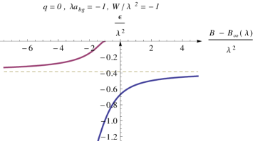
Figure 1: Bound states across a finite width Feshbach resonance in a spherical gauge field: For $B\gg B_{\infty}(\lambda)$, there is a single bound state due to the background scattering length. For $B\ll B_{0}(\lambda)$, there is a deep state corresponding to the closed channel boson, and an open channel bound state corresponding, again, to the background scattering length. The magnetic field regime around $B=B_{0}(\lambda)$ is interesting, with two bound states. The dashed line corresponds to the energy of the bound state $-E_{b}({a}_{bg})$ (see eqn. (14)) with an energy independent scattering length ${a}_{bg}$.

While the results derived above are valid for a generic gauge field, in particular those realized in recent experimentsWang et al. (2012); Cheuk et al. (2012), we now discuss Feshbach resonance in the spherical gauge fieldVyasanakere and Shenoy (2011) where many analytical results are possible. This gauge field results in an isotropic Rashba spin orbit coupling such that $H_{\sigma\sigma^{\prime}}=-\delta_{\sigma\sigma^{\prime}}\frac{\mbox{\boldmath$\nabla$}^{2}}{2}+i\lambda\mbox{\boldmath$\nabla$}\cdot\mbox{\boldmath$\tau$}_{\sigma\sigma^{\prime}}$, where $\tau$ is the vector of Pauli matrices. For an energy independent scattering length $a_{s}$, two particles always have a bound stateVyasanakere and Shenoy (2011) with binding energy

$$E_{b}(a_{s})=\frac{1}{4}\left(\frac{1}{a_{s}}+\sqrt{\frac{1}{a_{s}^{2}}+4\lambda^{2}}\right)^{2},$$ (14)

and the rashbon binding energy is $\lambda^{2}$.

The singlet threshold for this gauge fieldVyasanakere and Shenoy (2012) has a very interesting character. For $q=|\bm{q}|\leq 2\lambda$, ${\varepsilon_{th}^{s}}(q,\lambda)=-\lambda^{2}$, i. e., independent of $q$, and $q>2\lambda$, the threshold increases with increasing $q$. Focussing on the regime $q<2\lambda$, we find from eqn. (12) that

$$B_{\infty}(q,\lambda)=B_{\infty}-\lambda^{2}-\frac{q^{2}}{4},$$ (15)

which clearly demonstrates the $q$-dependence of the Feshbach field. In the remainder of the paper, we will discuss the Feshbach resonance at $q=0$ in the spherical gauge field for which $\Pi(q=0,z)$ has a nice analytic expression

$$\Pi(z)=\frac{1}{4\pi}\left(\sqrt{-z}-\frac{\lambda^{2}}{\sqrt{-z}}\right).$$ (16)

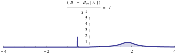
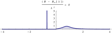
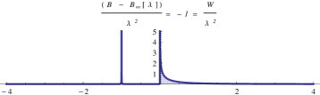
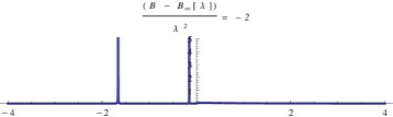
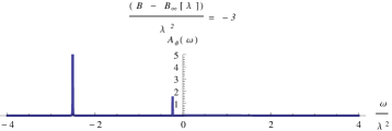
Figure 2: Evolution of the spectral function of the closed channel boson(CCB): Physical parameters are same as those in Fig. 1. For $B\gg B_{\infty}(\lambda)$, the CCB has most weight in the scattering continuum, while for $B\ll B_{0}(\lambda)$, the CCB does not significantly couple to the open channel. $B\sim B_{0}(\lambda)$ is of interest where the CCB has nearly equal weights in both the bound states.

Finite width resonance: We first consider a finite width resonance with a negative background scattering length. Fig. 1 shows the energy of the bound states as the magnetic field is swept across the resonance. When $B\gg B_{\infty}(\lambda)$ there is a single bound state which is open channel dominated. Indeed the energy of this state is slightly below the value given by eqn. (14) with $a_{s}={a}_{bg}$ (dashed line in Fig. 1) owing to the “level repulsion” with the closed channel boson. Quite interestingly, there is just this state at $B=B_{\infty}(\lambda)$. A second bound state appears only for $B<B_{0}(\lambda)$, and in the regime of magnetic field around $B_{0}(\lambda)$ the system supports two bound states. The bound state spectrum has the structure of an avoided crossing between the open channel bound state due to the background scattering length and the CCB. Further understanding of the physics can be obtained by a study of evolution of the spectral function of the CCB shown in fig. 2. For $B\gg B_{\infty}(\lambda)$, the CCB resides in the scattering continuum hybridizing with the open channel states. For $B\ll B_{0}(\lambda)$ the CCB decouples from the open channel (see lowest panel in fig. 2). What is noteworthy is that for $B\lessapprox B_{0}(\lambda)$, the CCB has nearly equal weight both the bound states. It will be interesting to explore systems where these two bound states are accessible, i. e., close in energy compared to, e. g., temperature.

A system with a positive background scattering length will also produce qualitatively similar physics. The notable difference is that the bound state induced by the background scattering length is deeper, and the two bound states induced by the resonance will be well separated and likely inaccessible in experiments.

We now turn to the possibility of realization of the rashbon state in a system with a resonance width comparable to the energy scale of the spin-orbit coupling ($\lambda^{2}$). Fig. 1 shows that the energy of the bound state at $B=B_{\infty}(\lambda)$ does not correspond to the rashbon energy of $-\lambda^{2}$. Furthermore, for $B\lesssim B_{\infty}(\lambda)$, the closed channel character of the bound state increases. It is therefore clear that the rashbon state is not realized across a finite width resonance (of width comparable to the energy scale of the spin orbit coupling).

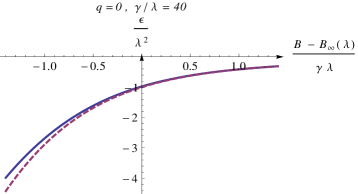
Figure 3: Bound state across the broad resonance in a spherical gauge field: Bound state energy of the single bound state (solid line), compared with the result (dashed line) based on an energy independent scattering length (eqn. (14)). Note that the rashbon state is realized at $B=B_{\infty}(\lambda)$.

Broad Feshbach Resonance: A broad resonance is obtained when ${a}_{bg}\rightarrow 0^{-}$ and $W\rightarrow-\infty$ keeping ${a}_{bg}W=\gamma$ finite. For a generic gauge field, in this limit, eqn. (8) becomes

$$\frac{1}{4\pi a_{r}(\bm{q},z)}=\frac{z-(B-B_{\infty}(\bm{q},{\bm{\lambda}}))}{4\pi\gamma}$$ (17)

and its energy dependence can be mitigated when $\gamma$ is large.

Fig. 3 shows the bound state spectrum for the spherical gauge field in a broad Feshbach resonance. The key point to be noted is that the system now has only one bound state. In fact, the bound state energy closely matches the energy obtained from eqn. (14) using $a_{s}$ as the scattering length at zero energy obtained from eqn. (17). What is heartening is that the bound state at $B=B_{\infty}(\lambda)$ does correspond to the rashbon state with weight dominantly in the open channel. Our study clearly points out that a broad resonance, i. e., whose width is much larger compared to the spin orbit coupling energy scale ($\lambda^{2}$), is the most favourable system to realize the rashbon.

Discussion: The results obtained here have many interesting consequences in the many body setting which we now discuss. Firstly, the $\bm{q}$ dependent shift of the Feshbach field should produce interesting effects in the many body system. On one hand, the effects of Pauli blocking inhibits bound state formation near $\bm{q}\approx{\bm{0}}$ (see Shenoy and Ho (2011)), while the effects of Pauli blocking are minimal for larger $\bm{q}$. On the other hand, the gauge field which promotes bound state formation at small $\bm{q}$ actually inhibits bound state formationVyasanakere and Shenoy (2012); Shenoy (2012); Zhang et al. (2012) at larger values of $\bm{q}$. The effect of the $\bm{q}$ dependent Feshbach field is therefore not obvious (atleast to the author) – this is clearly a very interesting problem for further investigation.

Although narrow resonances (width comparable to the spin orbit coupling scale) are not favourable for the realization of the rashbon, they do offer new possibilities. The regime of magnetic fields where there are two bound states is fertile with interesting new physics. In a low density system at low temperatures, the presence of the two bound states will promote fluctuations and possibly inhibit condensation – a study of this competition is also be an interesting direction for further investigation. The renormalizable field theory developed in this paper could be used for these investigations.

From the point of view of experiments, this work clearly points to the conditions favourable for the realization of the rashbon condensate. What is unequivocally clear from this work and the cited literature is that cold atoms in synthetic gauge fields is a treasure trove of interesting physics. We hope this motivates experimental efforts towards uncovering these.

Acknowledgement: This work is generously supported by DAE (SRC grant) and DST, India. The author is grateful to J. Vyasanakere for discussions, S. K. Ghosh and A. Agarwala for comments on the manuscript.

References

- Ketterle and Zwierlein (2008) W. Ketterle and M. W. Zwierlein, Nuovo Cimento Rivista Serie 31, 247 (2008).
- Bloch et al. (2008) I. Bloch, J. Dalibard, and W. Zwerger, Rev. Mod. Phys. 80, 885 (2008).
- Esslinger (2010) T. Esslinger, Annual Review of Condensed Matter Physics 1, 129 (2010).
- Cirac and Zoller (2012) J. I. Cirac and P. Zoller, Nature Physics 8, 264 (2012).
- Lin et al. (2009a) Y.-J. Lin, R. L. Compton, A. R. Perry, W. D. Phillips, J. V. Porto, and I. B. Spielman, Phys. Rev. Lett. 102, 130401 (2009a).
- Lin et al. (2009b) Y.-J. Lin, R. L. Compton, K. Jimenez-Garcia, J. V. Porto, and I. B. Spielman, Nature 462, 628 (2009b).
- Lin et al. (2011) Y.-J. Lin, K. Jimenez-Garcia, and I. B. Spielman, Nature 471, 83 (2011).
- Wang et al. (2012) P. Wang, Z.-Q. Yu, Z. Fu, J. Miao, L. Huang, S. Chai, H. Zhai, and J. Zhang, Phys. Rev. Lett. 109, 095301 (2012).
- Cheuk et al. (2012) L. W. Cheuk, A. T. Sommer, Z. Hadzibabic, T. Yefsah, W. S. Bakr, and M. W. Zwierlein, Phys. Rev. Lett. 109, 095302 (2012).
- Stanescu et al. (2008) T. D. Stanescu, B. Anderson, and V. Galitski, Phys. Rev. A 78, 023616 (2008).
- Wang et al. (2010) C. Wang, C. Gao, C.-M. Jian, and H. Zhai, Phys. Rev. Lett. 105, 160403 (2010).
- Ho and Zhang (2011) T.-L. Ho and S. Zhang, Phys. Rev. Lett. 107, 150403 (2011).
- Cong-Jun et al. (2011) W. Cong-Jun, I. Mondragon-Shem, and Z. Xiang-Fa, Chinese Physics Letters 28, 097102 (2011).
- Vyasanakere and Shenoy (2011) J. P. Vyasanakere and V. B. Shenoy, Phys. Rev. B 83, 094515 (2011).
- Vyasanakere et al. (2011) J. P. Vyasanakere, S. Zhang, and V. B. Shenoy, Phys. Rev. B 84, 014512 (2011).
- Yu and Zhai (2011) Z.-Q. Yu and H. Zhai, Phys. Rev. Lett. 107, 195305 (2011).
- Hu et al. (2011) H. Hu, L. Jiang, X.-J. Liu, and H. Pu, Phys. Rev. Lett. 107, 195304 (2011).
- Gong et al. (2011) M. Gong, S. Tewari, and C. Zhang, Phys. Rev. Lett. 107, 195303 (2011).
- Iskin and Subaş ı (2011) M. Iskin and A. L. Subaş ı, Phys. Rev. Lett. 107, 050402 (2011).
- Han and Sá de Melo (2012) L. Han and C. A. R. Sá de Melo, Phys. Rev. A 85, 011606 (2012).
- Vyasanakere and Shenoy (2012) J. P. Vyasanakere and V. B. Shenoy, New J. Phys. 14, 043041 (2012).
- Cui (2012) X. Cui, Phys. Rev. A 85, 022705 (2012).
- Zhang et al. (2012) P. Zhang, L. Zhang, and Y. Deng, Phys. Rev. A 86, 053608 (2012).
- Goldman et al. (2012) N. Goldman, W. Beugeling, and C. M. Smith, EPL (Europhysics Letters) 97, 23003 (2012).
- Dalibard et al. (2011) J. Dalibard, F. Gerbier, G. Juzeliūnas, and P. Öhberg, Rev. Mod. Phys. 83, 1523 (2011).
- Timmermans et al. (1999) E. Timmermans, P. Tommasini, M. Hussein, and A. Kerman, Physics Reports 315, 199 (1999).
- Chin et al. (2010) C. Chin, R. Grimm, P. Julienne, and E. Tiesinga, Rev. Mod. Phys. 82, 1225 (2010).
- Moerdijk et al. (1995) A. J. Moerdijk, B. J. Verhaar, and A. Axelsson, Phys. Rev. A 51, 4852 (1995).
- Kokkelmans et al. (2002) S. J. J. M. F. Kokkelmans, J. N. Milstein, M. L. Chiofalo, R. Walser, and M. J. Holland, Phys. Rev. A 65, 053617 (2002).
- Ho et al. (2012) T.-L. Ho, X. Cui, and W. Li, Phys. Rev. Lett. 108, 250401 (2012).
- Note (1) Generically, will also contain the magnetic field . While treating this is straightforward if cumbersome, we keep independent of the magnetic field for conceptual clarity.
- Timmermans et al. (2001) E. Timmermans, K. Furuya, P. W. Milonni, and A. K. Kerman, Physics Letters A 285, 228 (2001).
- Duine and Stoof (2004) R. Duine and H. Stoof, Physics Reports 396, 115 (2004).
- Braaten et al. (2008) E. Braaten, M. Kusunoki, and D. Zhang, Ann. Phys. 323, 1770 (2008).
- Liu et al. (2009) X.-J. Liu, M. F. Borunda, X. Liu, and J. Sinova, Phys. Rev. Lett. 102, 046402 (2009).
- Moody et al. (1989) J. Moody, A. Shapere, and F. Wilczek, in Geometric Phases in Physics, edited by A. Shapere and F. Wilczek (World Scientific, Singapore, 1989) pp. 160–183.
- Note (2) The necessary condition for the renormalizability is that where is the sign of the moment of the CCB. We have assumed (without loss of generality) that for our system, i. e., energy of the CCB increases with increasing .
- Zhou and Zhang (2012) K. Zhou and Z. Zhang, Phys. Rev. Lett. 108, 025301 (2012).
- Williams et al. (2012) R. A. Williams, L. J. LeBlanc, K. Jiménez-García, M. C. Beeler, A. R. Perry, W. D. Phillips, and I. B. Spielman, Science 335, 314 (2012).
- Vyasanakere and Shenoy (2012) J. P. Vyasanakere and V. B. Shenoy, Phys. Rev. A 86, 053617 (2012).
- Shenoy and Ho (2011) V. B. Shenoy and T.-L. Ho, Phys. Rev. Lett. 107, 210401 (2011).
- Shenoy (2012) V. B. Shenoy, ArXiv e-prints (2012), arXiv:1211.1831 [cond-mat.quant-gas] .
- Zhang et al. (2012) L. Zhang, Y. Deng, and P. Zhang, ArXiv e-prints (2012), arXiv:1211.6919 [cond-mat.quant-gas] .