The Partition Function of ABJ Theory

Abstract

We study the partition function of the ${\cal N}=6$ supersymmetric $U(N_{1})_{k}\times U(N_{2})_{-k}$ Chern-Simons-matter (CSM) theory, also known as the ABJ theory. For this purpose, we first compute the partition function of the $U(N_{1})\times U(N_{2})$ lens space matrix model exactly. The result can be expressed as a product of $q$-deformed Barnes $G$-function and a generalization of multiple $q$-hypergeometric function. The ABJ partition function is then obtained from the lens space partition function by analytically continuing $N_{2}$ to $-N_{2}$. The answer is given by ${\rm min}(N_{1},N_{2})$-dimensional integrals and generalizes the “mirror description” of the partition function of the ABJM theory, i.e. the ${\cal N}=6$ supersymmetric $U(N)_{k}\times U(N)_{-k}$ CSM theory. Our expression correctly reproduces perturbative expansions and vanishes for $|N_{1}-N_{2}|>k$ in line with the conjectured supersymmetry breaking, and the Seiberg duality is explicitly checked for a class of nontrivial examples.

1 Introduction

There has recently been remarkable progress in applications of the localization technique [1] to supersymmetric gauge theories, notably in dimensions $D\geq 3$: In $D=4$ the Seiberg-Witten prepotential of ${\cal N}=2$ supersymmetric QCD [2] was directly evaluated, and the partition functions and BPS Wilson loops of the ${\cal N}=2$ (and $2^{*}$) and ${\cal N}=4$ supersymmetric Yang-Mills theories (SYM) were reduced to eigenvalue integrals of the matrix model type [3], providing, in particular, a proof of the earlier results on a Wilson loop in the ${\cal N}=4$ SYM [4, 5]. In $D=3$ similar results were obtained for the partition functions and BPS Wilson loops of ${\cal N}=2$ supersymmetric Chern-Simons-matter (CSM) theories [6, 7], including the ${\cal N}=6$ superconformal theories constructed by Aharony, Bergman, Jafferis and Maldacena (ABJM) [8][9]. More recently, the localization technique was further applied to the partition functions of $5$-dimensional SYM with or without matter [10, 11, 12].

The localization method, resulting in the eigenvalue integrals of the matrix model type, allows us to obtain various exact results at strong coupling of supersymmetric gauge theories. In particular, these results provide useful data for the tests of the AdS/CFT correspondence [13] in the case of superconformal gauge theories. For instance, the precise agreement of the $N^{3/2}$ scaling between the free energy of the ABJ(M) theory [14, 15, 16] and its AdS₄ dual [8][9] is an important landmark that shows the power of the localization method in the context of AdS/CFT. Rather remarkably, exact agreements were also found in [17] between the $N^{5/2}$ scaling of 5d superconformal theories and that of their AdS₆ duals [18]. Furthermore, the tantalizing $N^{3}$ scaling of maximally supersymmetric 5d SYM was found in [12, 19] in line with the conjecture on $(2,0)$ 6d superconformal theory compactified on $S^{1}$ [20], despite thus far a lack of the precise agreement with its AdS₇ dual. It should, however, be noted that the utility of the localization method, unlike the integrability [21], is limited to a class of supersymmetric observables, such as the partition function and BPS Wilson loops. On the other hand, the localization method has an advantage over the integrability in that it can provide exact results at strong coupling beyond the large $N$ limit, where the integrability has not been as powerful.

In this paper we focus on the partition function of the ABJ theory, i.e., the ${\cal N}=6$ supersymmetric $U(N_{1})_{k}\times U(N_{2})_{-k}$ CSM theory, which generalizes the equal rank $N_{1}=N_{2}$ case of the ABJM theory [9]. Over the past few years there has been considerable progress in the study of the partition function and Wilson loops of the ABJM theory, whereas the ABJ case has not been as much understood. The ABJ generalization, for instance, has an important new feature, the Seiberg duality, which, however, lacks a full understanding. Besides being a generalization, it has recently been conjectured that the ABJ theory at large $N_{2}$ and $k$ with $N_{2}/k$ and $N_{1}$ fixed finite is dual to the ${\cal N}=6$ parity-violating Vasiliev higher spin theory on AdS₄ with $U(N_{1})$ gauge symmetry [22]. Thus a better understanding of the ABJ theory may provide valuable insights into the relation between higher spin particles and strings. It is therefore worth studying the partition function of the ABJ theory in great detail.

As mentioned above, the partition function of the ABJM theory has been well studied. In the large $N$ limit, the planar free energy has been computed, revealing the aforementioned $N^{3/2}$ scaling [14, 15, 16]. In fact, the result in [14, 15] is exact in ’t Hooft coupling $\lambda=N/k$ and, in particular, confirms a gravity prediction of the AdS radius shift in [23]. The planar result is not limited to the ABJM case; Drukker-Mariño-Putrov’s results include the partition function and Wilson loops of the ABJ theory, and the ABJ version of the radius shift [24] is also confirmed. In the meantime, beyond the large $N$ limit, the $1/N$ corrections of the ABJM partition function were summed up to all orders by solving the holomorphic anomaly equations of [25, 14, 26] at large $\lambda$ in the type IIA regime $k\gg 1$, and the result turned out to be simply an Airy function [27]. Subsequently, Mariño and Putrov developed a more elegant approach, the Fermi gas approach, without making any use of the matrix model techniques or the holomorphic anomaly equations, to compute directly the partition functions of ${\cal N}=3$ and ${\cal N}=2$ CSM theories including the ABJM theory [29, 30]. They found, in particular, a universal Airy function behavior for the ${\cal N}=3$ theories at large $N$ in the small $k$ M-theory regime. These non-planar results were reaffirmed by numerical studies in the case of the ABJM theory [31]. Furthermore, the Fermi gas approach was applied to the Wilson loops, exhibiting again the Airy function behavior [32]. Meanwhile, a number of exact computations of the ABJM partition function were carried out for various values of $N$ and $k$ [33, 34, 35]. It should also be noted that the nonperturbative effects ${\cal O}(e^{-N})$ of the M- and D-brane type can be systematically studied both in the matrix model [26] and the Fermi gas approaches [29].

In the unequal rank $N_{1}\neq N_{2}$ case of the ABJ theory, the Fermi gas approach thus far has not been applicable, and the study of finite $N_{1}$ and $N_{2}$ corrections to the ABJ partition function has not been as much developed as in the ABJM case. In this paper, we wish to lay the ground for the study of the ABJ partition function at finite $N_{1}$ and $N_{2}$. To this end, we first compute the partition function of the L(2,1) lens space matrix model [36, 37] exactly. By making use of the relation between the lens space and the ABJ matrix models [38], we map the lens space partition function to that of the ABJ matrix model by analytically continuing $N_{2}$ to $-N_{2}$. With our particular prescription of the analytic continuation, the final answer for the ABJ partition function is given by ${\rm min}(N_{1},N_{2})$-dimensional integrals and generalizes the “mirror description” of the partition function of the ABJM theory [39]. Our result may thus serve as the starting point for the ABJ generalization of the Fermi gas approach. Meanwhile, we test our prescription against perturbative expansions as well as the Seiberg duality conjecture of [9] and find that our final answer perfectly meets the expectations.

The rest of the paper is organized as follows: In Section 2 we outline our strategy for the calculations of the ABJ partition function and summarize the main result at each pivotal step of the computations. Most of the computational details are relegated to rather extensive appendices. In Section 3 we present a few simple examples of our results in order to elucidate otherwise rather complicated general results. In Section 4 we state the result of perturbative and nonperturbative checks that we carried out and illustrate with a few simple examples how they were actually done. Section 5 is devoted to the conclusions and the discussions.

2 The outline of calculations and main results

We are going to compute the partition function of the $U(N_{1})_{k}\times U(N_{2})_{-k}$ ABJ theory in the matrix model form [6, 7] obtained by the localization technique [3]:

$$Z_{\rm ABJ}(N_{1},N_{2})_{k}={\cal N}_{\rm ABJ}\int\prod_{i=1}^{N_{1}}{d\mu_{i}\over 2\pi}\prod_{a=1}^{N_{2}}{d\nu_{a}\over 2\pi}{\Delta_{\rm sh}(\mu)^{2}\Delta_{\rm sh}(\nu)^{2}\over\Delta_{\rm ch}(\mu,\nu)^{2}}e^{-{1\over 2g_{s}}\left(\sum_{i=1}^{N_{1}}\mu_{i}^{2}-\sum_{a=1}^{N_{2}}\nu_{a}^{2}\right)}\ ,$$ (2.1)

where the $\Delta_{\rm sh}$ factors are the one-loop determinants of the vector multiplets

$$\Delta_{\rm sh}(\mu)=\prod_{1\leq i<j\leq N_{1}}\left(2\sinh\left({\mu_{i}-\mu_{j}\over 2}\right)\right)\ ,\quad\Delta_{\rm sh}(\nu)=\prod_{1\leq a<b\leq N_{2}}\left(2\sinh\left({\nu_{a}-\nu_{b}\over 2}\right)\right)\ ,$$ (2.2)

and the $\Delta_{\rm ch}$ factor is the one-loop determinant of the matter multiplets in the bi-fundamental representation

$$\Delta_{\rm ch}(\mu,\nu)=\prod_{i=1}^{N_{1}}\prod_{a=1}^{N_{2}}\left(2\cosh\left({\mu_{i}-\nu_{a}\over 2}\right)\right)\ .$$ (2.3)

The string coupling $g_{s}$ is related to the Chern-Simons level $k\in\mathbb{Z}_{\neq 0}$ by

$$g_{s}={2\pi i\over k}\ ,$$ (2.4)

and the factor ${\cal N}_{\rm ABJ}$ in front is the normalization factor [15]

$${\cal N}_{\rm ABJ}:={i^{-{\kappa\over 2}(N_{1}^{2}-N_{2}^{2})}\over N_{1}!N_{2}!}\ ,\qquad\kappa:=\mathop{\mathrm{sign}}\nolimits k\ .$$ (2.5)

Note that, because of the relation

$$Z_{\rm ABJ}(N_{2},N_{1})_{k}=Z_{\rm ABJ}(N_{1},N_{2})_{-k}\ ,$$ (2.6)

we can assume $N_{1}\leq N_{2}$ without loss of generality.

2.1 The outline of calculations

Before going into the details of calculations, we shall first lay out our technical strategy: We adopt the idea employed in the large $N$ analysis of the ABJ(M) matrix model in [14, 15]. Namely, instead of performing the integrals in (2.1) directly,

1. we first compute the partition of the L(2,1) lens space matrix model [36, 37]

   $$Z_{\rm lens}(N_{1},N_{2})_{k}={\cal N}_{\rm lens}\int\prod_{i=1}^{N_{1}}{d\mu_{i}\over 2\pi}\prod_{a=1}^{N_{2}}{d\nu_{a}\over 2\pi}\Delta_{\rm sh}(\mu)^{2}\Delta_{\rm sh}(\nu)^{2}\Delta_{\rm ch}(\mu,\nu)^{2}e^{-{1\over 2g_{s}}\left(\sum_{i=1}^{N_{1}}\mu_{i}^{2}+\sum_{a=1}^{N_{2}}\nu_{a}^{2}\right)}$$ (2.7)

   with the normalization factor

   $${\cal N}_{\rm lens}={i^{-{\kappa\over 2}(N_{1}^{2}+N_{2}^{2})}\over N_{1}!N_{2}!}\ .$$ (2.8)

   
   

2. then analytically continue $N_{2}$ to $-N_{2}$ to obtain the partition function of ABJ theory [38]

   $$Z_{\rm ABJ}(N_{1},N_{2})_{k}=\lim_{\epsilon\to 0}\,{\cal C}(N_{2},\epsilon)Z_{\rm lens}(N_{1},-N_{2}+\epsilon)_{k}\ ,$$ (2.9)

where the proportionality constant is given in terms of the Barnes $G$-function $G_{2}(z)$,

$${\cal C}(N_{2},\epsilon)=(2\pi)^{-N_{2}}{G_{2}(N_{2}+1)\over G_{2}(-N_{2}+1+\epsilon)}\ .$$ (2.10)

A key observation is that the partition function (2.7) of the lens space matrix model is a sum of Gaussian integrals and can thus be calculated exactly in a very elementary manner. The analytic continuation $N_{2}\to-N_{2}$, on the other hand, is ambiguous and not as straightforward as one might expect. We find the appropriate prescription for the analytic continuation in two steps:

1. In the first step we propose a natural prescription that correctly reproduces, after a generalized $\zeta$-function regularization, the known perturbative expansions in the string coupling $g_{s}$. The resulting expression, however, is a formal series that is non-convergent and singular when $k$ is an even integer.

2. To circumvent these issues, in the second step, we introduce an integral representation which renders a formal series perfectly well-defined.

In other words, the integral representation (A) implements a generalized $\zeta$-function regularization automatically and (B) provides an analytic continuation in the complex parameter $g_{s}$ for the formal series.

As we will see later, the final answer in the integral representation passes perturbative as well as some nonperturbative tests and generalizes the “mirror description” [39] of the partition function of the ABJM theory to the ABJ theory.

2.2 The main results

We present, without much detail of derivations, the main result at each step of the outlined calculations. Most of the technical details will be given in the appendices.

$\bullet$ The lens space matrix model

As emphasized above, the lens space partition function (2.7) is a sum of Gaussian integrals and can be calculated exactly:

$$Z_{\text{lens}}(N_{1},N_{2})_{k} =i^{-{\kappa\over 2}(N_{1}^{2}+N_{2}^{2})}\left({g_{s}\over 2\pi}\right)^{N\over 2}q^{-{1\over 3}N(N^{2}-1)}$$

$$\qquad\times\sum_{({\cal N}_{1},\,{\cal N}_{2})}\prod_{C_{j}<C_{k}}(q^{C_{j}}-q^{C_{k}})\prod_{D_{a}<D_{b}}(q^{D_{a}}-q^{D_{b}})\prod_{C_{j},D_{a}}(q^{C_{j}}+q^{D_{a}})\ ,$$ (2.11)

where

$$q:=e^{-g_{s}}=e^{-{2\pi i\over k}},\qquad N=N_{1}+N_{2}.$$ (2.12)

The symbol $({\cal N}_{1},\,{\cal N}_{2})$ denotes the partition of the numbers $(1,2,\cdots,N)$ into two groups ${\cal N}_{1}=(C_{1},C_{2},\cdots,C_{N_{1}})$ and ${\cal N}_{2}=(D_{1},D_{2},\cdots,D_{N_{2}})$ where $C_{i}$’s and $D_{a}$’s are ordered as $C_{1}<\cdots<C_{N_{1}}$ and $D_{1}<\cdots<D_{N_{2}}$. The computation proceeds in two steps: (1) Gaussian integrals and (2) sums over permutations. The detailed derivation can be found in Appendix B.

As advertised, the result (2.11) can be written as a product of $q$-deformed Barnes $G$-function and a generalization of multiple $q$-hypergeometric function:

$$Z_{\text{lens}}(N_{1},N_{2})_{k} =i^{-{\kappa\over 2}(N_{1}^{2}+N_{2}^{2})}\left({g_{s}\over 2\pi}\right)^{N\over 2}q^{-{1\over 6}N(N^{2}-1)}(1-q)^{{1\over 2}N(N-1)}G_{2}(N+1;q)\,S(N_{1},N_{2})\ ,$$ (2.13)

where

$$S(N_{1},N_{2})=\sum_{({\cal N}_{1},\,{\cal N}_{2})}\prod\limits_{C_{j}<D_{a}}{q^{C_{j}}+q^{D_{a}}\over q^{C_{j}}-q^{D_{a}}}\prod\limits_{D_{a}<C_{j}}{q^{D_{a}}+q^{C_{j}}\over q^{D_{a}}-q^{C_{j}}}\ .$$ (2.14)

The $q$-deformed Barnes $G$-function $G_{2}(z;q)$ is defined in Appendix A and, as will be elaborated later, $S(N_{1},N_{2})$ is a generalization of multiple $q$-hypergeometric function. Recalling that $q=e^{-g_{s}}$, it is rather fascinating to observe that the string coupling $g_{s}$ is not only the loop-expansion parameter in quantum mechanics but also a quantum deformation parameter of special functions.

In Section 3 we will give simple examples of the lens space partition function in order to elucidate the $q$-hypergeometric structure.

$\bullet$ The ABJ theory

The next step in our strategy is the analytic continuation $N_{2}\to-N_{2}$ which maps the partition function of the lens space matrix model to that of the ABJ theory. For this purpose, we find it convenient to work with the second expression of the lens space partition function (2.13). Our claim is that the analytic continuation yields the following expression for the ABJ partition function in a formal series

$$Z_{\rm ABJ}(N_{1},N_{2})_{k} =i^{-{\kappa\over 2}(N_{1}^{2}+N_{2}^{2})}(-1)^{{1\over 2}N_{1}(N_{1}-1)}\,2^{-N_{1}}\,\left({g_{s}\over 2\pi}\right)^{N_{1}+N_{2}\over 2}(1-q)^{M(M-1)\over 2}G_{2}(M+1;q)$$

$$\quad\times{1\over N_{1}!}\sum\limits_{s_{1},\dots,s_{N_{1}}\geq 0}(-1)^{s_{1}+\cdots+s_{N_{1}}}\prod\limits_{j=1}^{N_{1}}{(q^{s_{j}+1})_{M}\over(-q^{s_{j}+1})_{M}}\prod\limits_{j<k}^{N_{1}}{(1-q^{s_{k}-s_{j}})^{2}\over(1+q^{s_{k}-s_{j}})^{2}}\ .$$ (2.15)

where we defined $M=N_{2}-N_{1}$ (for $N_{2}>N_{1})$ and $(a)_{n}$ is a shorthand notation for the $q$-Pochhammer symbol $(a;q)_{n}$ defined in Appendix A. We used an $\epsilon$-prescription in continuing $N_{2}$ to $-N_{2}$, as explained in detail in Appendix C.2.

However, as noted above, there are in principle multiple ways to continue $N_{2}$ to $-N_{2}$. It thus requires a particular prescription to fix this ambiguity. Our prescription is to continue $N_{2}$ to $-N_{2}$ with $S(N_{1},N_{2})$ written in the form

$$S(N_{1},N_{2})=\gamma(N_{1},N_{2})\Psi(N_{1},N_{2})$$ (2.16)

where

$$\gamma(N_{1},N_{2}) =(-1)^{{1\over 2}N_{1}(N_{1}-1)}\prod_{j=1}^{N_{1}-1}{(-q)_{j}^{2}\over(q)_{j}^{2}}\prod_{j=1}^{N_{1}}{(-q^{j})_{N_{2}}(-q^{j})_{-N_{1}-N_{2}}\over(q^{j})_{N_{2}}(q^{j})_{-N_{1}-N_{2}}}\ ,$$ (2.17)

$$\Psi(N_{1},N_{2}) ={1\over N_{1}!}\sum_{s_{1},\dots,s_{N_{1}}\geq 0}(-1)^{s_{1}+\cdots+s_{N_{1}}}\prod_{j=1}^{N_{1}}{(q^{s_{j}+1})_{-N_{1}-N_{2}}\over(-q^{s_{j}+1})_{-N_{1}-N_{2}}}\prod_{1\leq j<k\leq N_{1}}{(q^{s_{k}-s_{j}})_{1}^{2}\over(-q^{s_{k}-s_{j}})_{1}^{2}}\ .$$ (2.18)

As will be explained more in detail in Appendix C, there are a number of ways to express $S(N_{1},N_{2})$ that could yield different results after the analytic continuation: The range of the sum in (2.14) runs from $1$ to $N=N_{1}+N_{2}$. In order to make sense of analytic continuation in $N_{2}(>N_{1})$, the finite sum (2.14) is extended to the infinite sum (2.18). In fact, the summand for $s_{i}>N-1$ in (2.16) vanishes after an appropriate regularization. Now the point is that these vanishing terms could yield nonvanishing contributions after the analytic continuation. Clearly, the way to extend the finite sums to infinite ones is not unique, and this is where the ambiguity lies.

Our guideline for the correct prescription is to successfully reproduce the perturbative expansions in $g_{s}$. Indeed, it can be checked that the formal series (2.15) has the correct perturbative expansions, as we will discuss more in Section 4.1.

$\bullet$ The integral representation

As alluded to in the outline, the result (2.15) is not the final answer. It is a formal series that is non-convergent and singular when $k$ is an even integer. It can be rendered perfectly well-defined by introducing an integral representation: Specifically, our final answer for the analytic continuation is

$$Z_{\rm ABJ}(N_{1},N_{2})_{k} =i^{-{\kappa\over 2}(N_{1}^{2}+N_{2}^{2})}(-1)^{{1\over 2}N_{1}(N_{1}-1)}\,2^{-N_{1}}\,\left({g_{s}\over 2\pi}\right)^{N_{1}+N_{2}\over 2}(1-q)^{M(M-1)\over 2}G_{2}(M+1;q)$$

$$\quad\times{1\over N_{1}!}\prod_{j=1}^{N_{1}}\left[{-1\over 2\pi i}\int_{I}{\pi\,ds_{j}\over\sin(\pi s_{j})}\right]\prod_{j=1}^{N_{1}}{(q^{s_{j}+1})_{M}\over(-q^{s_{j}+1})_{M}}\prod_{1\leq j<k\leq N_{1}}{(1-q^{s_{k}-s_{j}})^{2}\over(1+q^{s_{k}-s_{j}})^{2}}\ ,$$ (2.19)

where $M=N_{2}-N_{1}$ (for $N_{2}>N_{1}$) and the integration range $I=\left[-i\infty-\eta,+i\infty-\eta\right]$ with $\eta>0$. We note that there is a subtlety in the choice of $\eta$: For example, when the string coupling $g_{s}$ takes the actual value of our interest, ${2\pi i\over k}$ with an integer $k$, as we will elaborate in Section 4.2, the parameter $\eta$ should be varied so that the partition function remains analytic in $k$, as one decreases the value of $k$ from the small coupling regime $|g_{s}|=|2\pi i/k|\ll 1$.

Although we lack a first principle derivation of the integral representation, we can give heuristic arguments as follows: First, this integral representation “agrees” with the formal series (2.15) order by order in the perturbative $g_{s}$-expansions. The integrals could be evaluated by considering the closed contours $C_{j}$ composed of the vertical line $I$ and the infinitely large semi-circle $C_{j}^{\infty}$ on the right half of the complex $s_{j}$-plane, if the contribution from $C_{j}^{\infty}$ were to vanish; see Figure 1. In the $g_{s}$-expansions, the poles would only come from the factors $1/\sin(\pi s_{j})$ and are at $s_{j}=n_{j}\in\mathbb{Z}_{\geq 0}$. Thus the residue integrals would correctly reproduce (2.15). In actuality, however, the contribution from $C_{j}^{\infty}$ does not vanish, and thus this argument is heuristic at best; we will see precisely how the $g_{s}$-expansions work in an example in section 4.1. We note that, to the same degree of imprecision, the integral representation (2.19) can be thought of as the Sommerfeld-Watson transform of (2.15).

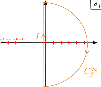
Figure 1: “The integration contour” $C_{j}=I+C_{j}^{\infty}$ for the perturbative ABJ partition function: The only perturbative (P) poles are indicated by red “$+$”. See text for detail.

Second, as implied in the first point, the integral representation (2.19) provides a “nonperturbative completion” for the formal series (2.15). In fact, nonperturbatively, there appear additional poles from the factors $1/(-q^{s_{j}+1})_{M}$ and $1/(1+q^{s_{k}-s_{j}})^{2}$ in the contour integrals. They are located at $s_{j}=-{(2n+1)\pi i\over g_{s}}-m$ and $s_{j}=-{(2n+1)\pi i\over g_{s}}+s_{k}$ with $n\in\mathbb{Z}$ and $m=1,\cdots,M$, as shown in Figure 2. Their residues are of order $e^{1/g_{s}}$. Hence these can be regarded as nonperturbative (NP) poles, whereas the previous ones are perturbative (P) poles. Again, these statements are rather heuristic, and we will see how precisely P and NP poles contribute to the contour integral in Section 4.2.

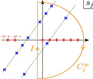
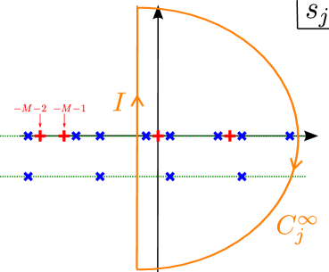
Figure 2: The nonperturbative (NP) poles are added and indicated by blue “$\times$”. The left panel corresponds to the complex $g_{s}$ case. The right panel is the actual case of our interest $g_{s}=2\pi i/k$. (Shown is the case $k=3$ and $M=3$.)

A few remarks are in order:

1. As promised, there is no issue of convergence in the expression (2.19). It is also well-defined in the entire complex $q$-plane. The integrand becomes singular for $q=e^{-2\pi i/k}$ with even integer $k$ as in the formal series (2.15). However, this merely represents pole singularities and yields finite residue contributions.

2. It should be noted that our main result (2.19) lacks a first principle derivation. It thus requires a posteriori justification. On this score, as stressed and will be discussed more in Section 4.1, the integral representation (2.19) correctly reproduces the perturbative expansions; moreover, it automatically implements a generalized $\zeta$-function regularization needed in the perturbative expansions of the infinite sum (2.15). Meanwhile, a successful test of the Seiberg duality conjectured in [9] provides evidence for our proposed nonperturbative completion. We will explicitly show a few nontrivial examples of the Seiberg duality at work in Section 4.2.

3. In the ABJM limit ($M=0$), the integral representation (2.19) coincides with the “mirror description” of the ABJM partition function found in [39]. This provides a further support for our prescription and implies that we have found a generalization of the “mirror description” in the case of the ABJ theory. Our finding may thus serve as the starting point for the generalization of the Fermi gas approach developed in [29] to the ABJ theory.

4. One of the ABJ conjectures is that the ${\cal N}=6$ $U(N_{1})_{k}\times U(N_{1}+M)_{-k}$ theory with $M>k$ may not exist as a unitary theory [9]. It is further expected that the supersymmetries are spontaneously broken in this case [40] (see also [41]). A manifestation of this conjecture is that the partition function (2.19) vanishes when $M>k$ because

   $$(1-q)^{{M(M-1)\over 2}}G_{2}(M+1;q)=\prod_{j=1}^{M-1}(q)_{j}=0\quad\mbox{for}\quad q=e^{-{2\pi i\over k}}\ .$$ (2.20)

   Note that the $q$-deformed Barnes $G$-function $G_{2}(M+1;q)$ is precisely a factor that appears in the partition function of the $U(M)_{k}$ Chern-Simons theory. We thus expect that this property is not peculiar to the ${\cal N}=6$ CSM theories but holds for CSM theories with less supersymmetries as long as they contain the $U(M)_{k}$ CS theory as a subsector.

3 Examples

In this section we present a few simple examples of the lens space and ABJ partition functions in order to get the feel of the expressions found in the previous section. In particular, these examples clarify the appearance of $q$-hypergeometric functions in the lens space partition function and how they are mapped to in the ABJ partition function. We also provide a simplest example of the exact ABJ partition function.

$\bullet$ The CS matrix model

The first example is the simplest case, the $N_{1}=0$ or $N_{2}=0$ case, which corresponds to the Chern-Simons matrix model. From (2.13) one immediately finds for the $U(M)_{k}$ CS theory that

$$Z_{\rm CS}(M)_{k}=Z_{\rm lens}(M,0)_{k}=i^{-{\kappa M(M-1)\over 2}}|k|^{-{M\over 2}}q^{-{M(M^{2}-1)\over 6}}(1-q)^{{1\over 2}M(M-1)}G_{2}(M+1;q)\ .$$ (3.1)

Note that this takes the more familiar form [42, 43] (without the level shift) if one uses the formula

$$i^{-{\kappa M(M-1)\over 2}}(1-q)^{{1\over 2}M(M-1)}G_{2}(M+1;q)=q^{{M(M^{2}-1)\over 12}}\prod_{j=1}^{M-1}\left(2\sin{\pi j\over|k|}\right)^{M-j}\ .$$ (3.2)

It should now be clear that the $q$-deformed Barnes $G$-function is a contribution from the $U(|N_{1}-N_{2}|)_{k}$ pure CS subsector in the $U(N_{1})_{k}\times U(N_{2})_{-k}$ theory.

$\bullet$ The lens space matrix model

The next simplest example is the $N_{1}=1$ case studied in detail in Appendix C.2.1. From (2.13) together with (C.28) and (C.29), the $U(1)_{k}\times U(N_{2})_{-k}$ lens space partition function yields

$$Z_{\text{lens}}(1,N_{2})_{k}=\, i^{-{\kappa\over 2}(N_{2}^{2}+1)}\left({g_{s}\over 2\pi}\right)^{N_{2}+1\over 2}q^{-{N_{2}(N_{2}+1)(N_{2}+2)\over 6}}(1-q)^{N_{2}(N_{2}+1)\over 2}G_{2}(N_{2}+2;q)$$

$$\times{(-q)_{N_{2}}\over(q)_{N_{2}}}\,_{2}\phi_{1}\left({q^{-N_{2}},-q\atop-q^{-N_{2}}};q,-1\right)\ ,$$ (3.3)

where the special function $\,{}_{2}\phi_{1}=\Phi(1,N_{2})$ is a $q$-hypergeometric function [44] whose definition is given in Appendix A. Intriguingly, the whole function $S(1,N_{2})$ in the second line is essentially an orthogonal $q$-polynomial, the continuous $q$-ultraspherical (or Rogers) polynomial [45], and very closely related to Schur Q-polynomials [46].

The next example is the $N_{1}=2$ case discussed in detail in Appendix C.2.2. In parallel with the previous case, from (2.13) together with (C.41) and (C.42), one finds the $U(2)_{k}\times U(N_{2})_{-k}$ lens space partition function

$$Z_{\text{lens}}(2,N_{2})_{k} =i^{-{\kappa\over 2}(N_{2}^{2}+4)}\left({g_{s}\over 2\pi}\right)^{N_{2}+2\over 2}q^{-{(N_{2}+1)(N_{2}+2)(N_{2}+3)\over 6}}(1-q)^{(N_{2}+1)(N_{2}+2)\over 2}G_{2}(N_{2}+3;q)$$

$$\times{(-q)_{N_{2}}(-q^{2})_{N_{2}}\over(q)_{N_{2}}(q^{2})_{N_{2}}}\,\Phi^{2:2;4}_{2:1;3}\!\left(\begin{array}[]{c@{~}c@{~}c@{~}c@{~}c}q^{-N_{2}},-q^{2}\hfil~{}&:\hfil~{}&q^{-N_{2}-1},-q\hfil~{}&;\hfil~{}&q^{2},q^{2},-q,-q\\ -q^{-N_{2}},q^{2}\hfil~{}&:\hfil~{}&-q^{-N_{2}-1}\hfil~{}&;\hfil~{}&-q^{2},-q^{2},q\end{array};~{}q~{};1,-1\right)\ ,$$ (3.6)

where the special function $\Phi^{2:2;4}_{2:1;3}=\Phi(2,N_{2})$ is a double $q$-hypergeometric function defined in Section 10.2 of [44].

As promised, these examples elucidate that the function $S(N_{1},N_{2})$ defined in (2.14) is a generalization of multiple $q$-hypergeometric function.

$\bullet$ The ABJ theory

We now present the ABJ counterpart of the previous two examples. Although we have placed great emphasis on the $q$-hypergeometric structure of the lens space partition function, we have not found a way to take full advantage of this fact in understanding the ABJ partition function thus far.

In the meantime, as mentioned in the previous section and discussed in great detail in Appendix C.2, we find the expression (C.56) more convenient for performing the analytic continuation $N_{2}\to-N_{2}$ than the $q$-hypergeometric representation (C.52). The end result is presented in (2.19). In the case of the $U(1)_{k}\times U(N_{2})_{-k}$ ABJ partition function, one finds

$$Z_{\rm ABJ}(1,N_{2})_{k}=\, {1\over 2}\,q^{{1\over 12}N_{2}(N_{2}-1)(N_{2}-2)}|k|^{-{N_{2}+1\over 2}}\prod_{j=1}^{N_{2}-2}\left(2\sin{\pi j\over|k|}\right)^{N_{2}-1-j}$$

$$\hskip 2.84544pt\times\left[{-1\over 2\pi i}\int_{I}{\pi\,ds\over\sin(\pi s)}\prod_{l=1}^{N_{2}-1}\tan\left({(s+l)\pi\over|k|}\right)\right]\ .$$ (3.7)

Similarly, the $U(2)_{k}\times U(N_{2})_{-k}$ ABJ partition function yields

$$Z_{\rm ABJ}(2,N_{2})_{k}=\, -{1\over 8}q^{{1\over 12}(N_{2}-1)(N_{2}-2)(N_{2}-3)}|k|^{-{N_{2}+2\over 2}}\prod_{j=1}^{N_{2}-3}\left(2\sin{\pi j\over|k|}\right)^{N_{2}-2-j}$$

$$\times\prod_{j=1}^{2}\left[{-1\over 2\pi i}\int_{I}{\pi\,ds_{j}\over\sin(\pi s_{j})}\prod_{l=1}^{N_{2}-2}\tan\left({(s_{j}+l)\pi\over|k|}\right)\right]\tan^{2}\left({(s_{2}-s_{1})\pi\over|k|}\right)\ .$$ (3.8)

Note that the $U(N_{1})_{k}\times U(N_{2})_{-k}$ ABJ theory with finite $N_{1}$ and large $N_{2}$ and $k$ is conjectured to be dual to ${\cal N}=6$ parity-violating Vasiliev higher spin theory on $AdS_{4}$ with $U(N_{1})$ gauge symmetry [47, 22]. It would thus be very interesting to study the large $N_{2}$ and $k$ limit of the $N_{1}=1$ and $2$ partition functions [48]. It may shed some lights on the understanding of the ${\cal N}=6$ parity-violating Vasiliev theory on $AdS_{4}$.

Finally, we provide a simplest example of the exact ABJ partition function, i.e., the $U(1)_{k}\times U(2)_{-k}$ case. The integral in (3.7) can be carried out by applying a similar trick to the one used in [33]. This yields

$$Z_{\rm ABJ}(1,2)_{k}=\, {1\over 2}\,|k|^{-{3\over 2}}\times\begin{cases}{1\over 2}\left[\sum_{n=1}^{|k|-1}(-1)^{n-1}\tan\bigl{(}{\pi n\over|k|}\bigr{)}+|k|(-1)^{|k|-1\over 2}\right]&\quad(k={\rm odd})\ ,\\[4.30554pt] \sum_{n=1}^{|k|-1}(-1)^{n-1}\left({1\over 2}-{n\over k}\right)\tan\bigl{(}{\pi n\over|k|}\bigr{)}&\quad(k={\rm even})\ .\end{cases}$$ (3.9)

It may be worth noting that the formal series (2.15) for the $U(1)_{k}\times U(2)_{-k}$ theory, albeit nonconvergent, can be expressed in a closed form after a regularization:

$$Z_{\rm ABJ}(1,2)_{k}=\, {1\over 2}\,i^{-\kappa}\,|k|^{-{3\over 2}}\left[{1\over 2}-{2\over\log q}\left(\log\left(1+q^{2}\over 1+q\right)+\psi_{q}(1)-2\psi_{q^{2}}(1)+\psi_{q^{4}}(1)\right)\right]\ ,$$ (3.10)

where $\psi_{q}(z)$ is a $q$-digamma function defined in Appendix A, and we used the regularization $\sum_{s=0}^{\infty}(-1)^{s}={1\over 2}$. This expression is, however, not well-defined for $q$ a root of unity and hence an integer $k$. On the other hand, this exemplifies the fact that the integral representation (2.19) provides an analytic continuation of the formal series (2.15) in the complex $q$-plane.

4 Checks

As mentioned in Section 2, our main result (2.19) lacks a first principle derivation. It thus requires a posteriori justification. In this section we show that our prescription passes perturbative as well as nonperturbative tests. We have, however, been unable to prove it in generality. Although our checks are on a case-by-case basis, we have examined several nontrivial cases that provide convincing evidence for our claim.

4.1 Perturbative expansions

The perturbative expansion of the lens space free energy is presented in [37]. In Appendix D, we extend their result to the order ${\cal O}(g_{s}^{8})$. We would like to see if the perturbative expansions of both (2.15) and (2.19) correctly reproduce this result with the replacement $N_{2}$ by $-N_{2}$. We have checked the cases $N_{1}=1$ and $N_{2}$ up to $8$, $N_{1}=2$ and $N_{2}$ up to $5$, $N_{1}=3$ and $N_{2}$ up to $5$, and $N_{1}=4$ and $N_{2}$ up to $4$, to the order ${\cal O}(g_{s}^{8})$ and found perfect agreements with the result in Appendix D. These checks are straightforward, and we will not spell out all the details. Instead, we describe only the essential points in the calculations and illustrate with a simple but nontrivial example how the checks were done in detail.

The formal series

In the case of the formal series (2.15), as remarked in the previous section, the perturbative expansion is correctly reproduced after the generalized $\zeta$-function regularization:

$$\sum_{s=0}^{\infty}(-1)^{s}s^{n}=\left\{\begin{array}[]{ll}{\rm Li}_{-n}(-1)=(2^{n+1}-1)\zeta(-n)=-{2^{n+1}-1\over n+1}B_{n+1}&\quad(\mbox{for}\quad n\geq 1)\ ,\\ 1+{\rm Li}_{0}(-1)={1\over 2}=-B_{1}&\quad(\mbox{for}\quad n=0)\ ,\end{array}\right.$$ (4.1)

where ${\rm Li}_{s}(z)$ is the polylogarithm and $B_{n}$ are the Bernoulli numbers. We show the detail of the $(N_{1},N_{2})=(2,3)$ example to illustrate how the generalized $\zeta$-function regularization yields the correct perturbative expansion to the order ${\cal O}(g_{s}^{4})$. In this case there are two infinite sums involved. Now, recall that the summand is a function of $q=\exp\left(-g_{s}\right)$. Expanding it as a power series in $g_{s}$ and using the regularization (4.1), one finds

The 2nd line of (2.15) $$={g_{s}^{4}\over 32}\left(\text{Li}^{2}_{-3,-1}\!-\!2\text{Li}^{2}_{-2,-2}\!+\!\text{Li}^{2}_{-1,-3}\right)\!-\!{g_{s}^{6}\over 384}\left(3\text{Li}^{2}_{-5,-1}\!-\!10\text{Li}^{2}_{-4,-2}\!+\!14\text{Li}^{2}_{-3,-3}\right.$$

$$\left.-10\text{Li}^{2}_{-2,-4}+3\text{Li}^{2}_{-1,-5}\right)+{g_{s}^{8}\over 23040}\left(33\text{Li}^{2}_{-7,-1}-154\text{Li}^{2}_{-6,-2}+336\text{Li}^{2}_{-5,-3}\right.$$

$$\left.-430\text{Li}^{2}_{-4,-4}+336\text{Li}^{2}_{-3,-5}-154\text{Li}^{2}_{-2,-6}+33\text{Li}^{2}_{-1,-7}\right)+{\cal O}(g_{s}^{10})$$

$$=-\frac{1}{512}g_{s}^{4}-\frac{19}{12288}g_{s}^{6}-\frac{137}{81920}g_{s}^{8}+{\cal O}(g_{s}^{10})\ ,$$ (4.2)

where we abbreviated the product ${\rm Li}_{-n_{1}}(-1){\rm Li}_{-n_{2}}(-1)$ by ${\rm Li}^{2}_{-n_{1},-n_{2}}$. This yields

$$F_{\rm ABJ}(2,3)=\log Z_{\rm ABJ}(2,3)=\log\left[\frac{2^{-12}(2\pi g_{s})^{13\over 2}}{2^{-1}(2\pi)^{9}}\right]+\frac{19}{24}g_{s}^{2}+\frac{3127}{5760}g_{s}^{4}+{\cal O}(g_{s}^{6})$$ (4.3)

in agreement with the result in Appendix D with the replacement $N_{2}$ by $-N_{2}$. Note also that the tree contribution, the first logarithmic term, is in a precise agreement with (C.13).

The integral representation

The integral representation (2.19) does not require any regularization. Instead, the generalized $\zeta$-function regularization (4.1) is automatically implemented by the integral

$$-{1\over 2\pi i}\int_{I}{\pi ds\over\sin(\pi s)}s^{n}=-{2^{n+1}-1\over n+1}B_{n+1}\ ,$$ (4.4)

where $n\geq 0$. It follows immediately from this fact that

$$\text{the 2nd line of (\ref{ABJpart_integral})}=\text{the 2nd line of (\ref{ABJpart_formalsum})}$$ (4.5)

at all orders in the $g_{s}$-expansions. Hence the integral representation correctly reproduces the perturbative expansions.

4.2 The Seiberg duality

As emphasized before, the integral representation (2.19) provides a “nonperturbative completion” for the formal series (2.15). A way to test this claim is to see if the Seiberg duality conjectured in [9] holds. This duality is an equivalence between the two ABJ theories; schematically,

$$U(N_{1})_{k}\times U(N_{1}+M)_{-k}=U(N_{1}+|k|-M)_{k}\times U(N_{1})_{-k}\ .$$ (4.6)

We are going to show, in the simple but nontrivial case of $N_{1}=1$, that the partition functions of the dual pairs agree up to a phase. In fact, a proof of the Giveon-Kutasov duality including the ${\cal N}=6$ case was proposed in [56], which assumed one conjecture to be proven. In particular, their conjecture gives a formula for the phase differences of the dual pairs. We will explicitly confirm their claim in our examples below.

Seiberg duality for $\boldsymbol{N_{1}=1}$

For $N_{1}=1$, the duality relation (4.6) reads

$$U(1)_{k}\times U(N_{2})_{-k}=U(1)_{-k}\times U(2+|k|-N_{2})_{k}\ .$$ (4.7)

In this case, we can actually prove that the integral representation (2.19) indeed gives identical results for the dual pair, up to a phase. Let us rewrite the $(1,N_{2})$ partition function given in (3.7) in the following form

$$Z_{\rm ABJ}(1,N_{2})_{k} =(2|k|)^{-1}Z_{\rm CS}^{0}(N_{2}-1)_{k}\,I(1,N_{2})_{k}\,e^{i\theta(1,N_{2})_{k}}\ .$$ (4.8)

Here, $Z_{\rm CS}^{0}(M)_{k}$ is the Chern-Simons (CS) partition function

$$Z_{\rm CS}^{0}(M)_{k}=|k|^{-{M\over 2}}\prod_{j=1}^{M-1}\left(2\sin{\pi j\over|k|}\right)^{M-j}$$ (4.9)

which is essentially the same as (3.1) up to a phase due to difference in the framing [15]. Moreover,

$$I(1,N_{2})_{k}: =-{1\over 2\pi i}\int_{I}{\pi\,ds\over\sin(\pi s)}\prod_{l=1}^{N_{2}-1}\tan\left({(s+l)\pi\over|k|}\right)\ ,$$ (4.10)

$$\theta(1,N_{2})_{k} :=-{\pi\over 6k}N_{2}(N_{2}-1)(N_{2}-2).$$ (4.11)

We can show that $Z_{\rm CS}^{0}(N_{2}-1)_{k}$ and $I(1,N_{2})_{k}$ are separately invariant under the Seiberg duality while the phase factor $e^{i\theta(1,N_{2})_{k}}$ gives a phase that precisely agrees with the one given in [56].

First, the invariance of $Z_{\rm CS}^{0}(N_{2}-1)_{k}$ is nothing but the level-rank duality of the CS partition function, which means the identity $Z_{\rm CS}^{0}(M)_{k}=Z_{\rm CS}^{0}(|k|-M)_{k}$. It is straightforward to see that this implies that $Z_{\rm CS}^{0}(N_{2}-1)_{k}$ is invariant under the Seiberg duality (4.7). Second, the phase difference between the dual theories (4.7) is

$$\theta(1,N_{2})_{k}-\theta(1,2+|k|-N_{2})_{-k}=\pi\left[\kappa\left(-\frac{1}{6}k^{2}-\frac{1}{2}N_{2}^{2}+N_{2}-\frac{1}{3}\right)+\frac{1}{2}k(N_{2}-1)\right].$$ (4.12)

One can show that this phase difference is exactly the same as the one given in [56].

Now let us move on to the most nontrivial part, i.e., the invariance of the integral (4.10) under the Seiberg duality. One can show that, despite appearances, the integrand is actually the same function for the dual theories (4.7) up to a shift in $s$. Therefore, the contour integral gives the same answer for the duals, if the contour is chosen appropriately. As explained in section 2.2, the integrand has perturbative (P) poles coming from $\pi\over\sin(\pi s)$ and non-perturbative (NP) poles coming from the product factor $\prod_{l}\tan$. Although the integrand remains the same under the Seiberg duality, the interpretation of its poles gets interchanged; i.e., a P pole in the original theory is interpreted as a NP pole in the dual theory, and vice versa. We will see this explicitly in examples below, relegating the general proof to Appendix E.

The integrand of (4.10) is an antiperiodic (periodic) function with $s\cong s+|k|$ for odd (even) $k$, and the P and NP poles occur on the real $s$ axis in bunches with this periodicity. The prescription for the contour is to take it to go to the left of one of such bunches. In Appendix E, we show that this means that

$$\eta=\begin{cases}0_{+}&\qquad\text{if}\quad{|k|\over 2}-N_{2}+1\geq 0,\\ -{|k|\over 2}+N_{2}-1+0_{+}&\qquad\text{if}\quad{|k|\over 2}-N_{2}+1\leq 0.\\ \end{cases}$$ (4.13)

This is required for the Seiberg duality to work, but it is also necessary for the ABJ partition function to be analytic in $k$, which is clearly the case for the original expression (2.1). In the weak coupling regime $|g_{s}|=|2\pi i/k|\ll 1$, the NP poles are far away from the origin (distance $\sim 1/|g_{s}|\sim|k|$) and we can safely take $\eta=0_{+}$. However, as we decrease $|k|$ continuously, the NP poles come closer to the origin and, eventually, at some even $|k|$, one of the NP poles that was in the $s>0$ region reaches $s=0$. As we further decrease $|k|$ continuously, this NP pole enters the $s<0$ region. In order for the partition function to be analytic in $k$, one needs to increase the value of $\eta$ so that this NP pole does not move across the contour $I$ but stays to the right of it.

Odd $\boldsymbol{k}$ case

The integral (4.10) for odd $k$ is equal to the following contour integral

$$I(1,N_{2})_{k}=-{1\over 4\pi i}\int_{C}{\pi\,ds\over\sin(\pi s)}\prod_{l=1}^{N_{2}-1}\tan\left({(s+l)\pi\over|k|}\right)\ ,$$ (4.14)

where the integral contour $C$ is given by $C=I\cap I_{i\infty}\cap I_{k}\cap I_{-i\infty}$ (clockwise), where the contour $I_{k}$ is parallel to $I$ and shifted by $|k|$, and the contours $I_{i\infty}$ and $I_{-i\infty}$ are at infinity; see Figure 3. Note that the anti-periodicity of the integrand allows us to write the line integral (4.10) as a closed contour integral, but the contour is different from the tentative contour shown for the sake of sketchy illustration in Figures 1 and 2. By summing up pole residues inside $C$, one finds

$$I(1,N_{2})_{k} ={1\over 2}\biggl{[}\sum_{n=0}^{|k|-N_{2}}(-1)^{n}\prod_{j=1}^{N_{2}-1}\tan{\pi(n+j)\over|k|}-|k|(-1)^{|k|-1\over 2}\sum_{n=1}^{N_{2}-1}(-1)^{n}\prod_{\begin{subarray}{c}j=1\\ (\neq n)\end{subarray}}^{N_{2}-1}\tan{\pi({k\over 2}-n+j)\over|k|}\biggr{]}.$$ (4.15)

The first term comes from P poles and the second from NP poles. Although we prove the Seiberg duality in Appendix E, it is quite nontrivial that (4.15) gives the same value for the dual pair (4.7).

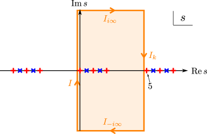
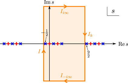
(a) $|k|=5,N_{2}=3$	(b) $|k|=5,N_{2}=4$
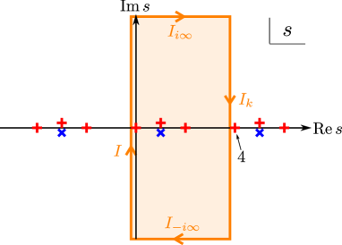
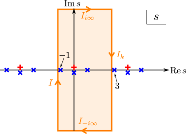
(c) $|k|=4,N_{2}=2$	(d) $|k|=4,N_{2}=4$

Figure 3: The integration contour $C=I\cap I_{i\infty}\cap I_{k}\cap I_{-i\infty}$ (clockwise) and poles, for various values of $k,N_{2}$. (a) and (b) are Seiberg duals of each other and so are (c) and (d). The contour $I_{k}$ is parallel to $I$ and shifted by $k$, and the contours $I_{i\infty}$ and $I_{-i\infty}$ are at infinity. “$+$” (red) denotes the P pole and “$\times$” (blue) the NP pole. Some poles and zeros are shown slightly above or below the real $s$ axis, but this is for the convenience of presentation and all poles and zeros are on the real $s$ axis. The choices of the parameter $\eta$ for the contour $I$ are $\eta=0_{+}$ for (a) and (c), $\eta={1\over 2}+0_{+}$ for (b), and $\eta=1+0_{+}$ for (d).

Let us look at this in more detail in the following case:

$$U(1)_{5}\times U(3)_{-5}=U(4)_{5}\times U(1)_{-5}\ .$$ (4.16)

Using the above formulas, we obtain the partition functions of this dual pair which can be massaged into

$$Z_{\rm ABJ}(1,3)_{5} ={1\over 50}\sin{\pi\over 5}\biggl{[}\underbrace{\tan{2\pi\over 5}\left(2\tan{\pi\over 5}+\tan{2\pi\over 5}\right)}_{\text{P}}\underbrace{-10\cot{\pi\over 5}}_{\text{NP}}\biggr{]}e^{-{\pi i\over 5}}\ ,$$ (4.17)

$$Z_{\rm ABJ}(1,4)_{-5} ={1\over 50}\sin{\pi\over 5}\biggl{[}\underbrace{-10\cot{\pi\over 5}}_{\text{P}}\underbrace{+\tan{2\pi\over 5}\left(2\tan{\pi\over 5}+\tan{2\pi\over 5}\right)}_{\text{NP}}\biggr{]}e^{4\pi i\over 5}\ .$$ (4.18)

These two indeed agree up to a phase and the phase difference agrees with the conjecture made in [56]. Observe that the contributions from the P and NP poles are interchanged under the duality. See Figure 3(a), (b) for the structure of the P and NP poles in the two theories. For discussion on the pole structure in more general cases, we refer the reader to Appendix E.

Even $\boldsymbol{k}$ case

The even $k$ case is technically a little more tricky. Using a trick similar to the one used in [33], the integral (4.10) for even $k$ can be shown to be equal to the following contour integral

$$I(1,N_{2})_{k}=-{1\over 2\pi i}\int_{C}{\pi\,ds\over\sin(\pi s)}\left(a-{s\over k}\right)\ \prod_{l=1}^{N_{2}-1}\tan\left({(s+l)\pi\over k}\right),$$ (4.19)

where $a$ is an arbitrary constant. For ${|k|\over 2}-N_{2}+1\geq 0$, we can evaluate this by summing over pole residues and obtain

$$I(1,N_{2})_{k}=\left(\sum_{n=0}^{{|k|\over 2}-N_{2}}+\sum_{n={|k|\over 2}}^{|k|-N_{2}}\right)\left(a-{n\over|k|}\right)(-1)^{n}\prod_{j=1}^{N_{2}-1}\tan{\pi(n+j)\over|k|}$$

$$\quad+\sum_{n=1}^{N_{2}-1}(-1)^{{|k|\over 2}-n}\left[-\left(a-{1\over 2}+{n\over|k|}\right)\sum_{\begin{subarray}{c}j=1\\ (j\neq n)\end{subarray}}^{N_{2}-1}{2\over\sin{2\pi\left({|k|\over 2}-n+j\right)\over|k|}}+{1\over\pi}\right]\prod_{\begin{subarray}{c}j=1\\ (j\neq n)\end{subarray}}^{N_{2}-1}\tan{\pi(n+j)\over|k|}.$$ (4.20)

The first line comes from P poles which are simple, while the second line comes from double poles created by simple NP and P poles sitting on top of each other. We note also that, despite its appearance, this expression does not depend on the constant $a$. The expression of $I(1,N_{2})_{k}$ for ${|k|\over 2}-N_{2}+1\leq 0$ is more lengthy and we do not present it, because the Seiberg duality proven in Appendix E guarantees that it can be obtained from (4.20).

Let us study in detail the following duality

$$U(1)_{4}\times U(2)_{-4}=U(4)_{4}\times U(1)_{-4}\ .$$ (4.21)

The partition functions of this dual pair yield

$$Z_{\rm ABJ}(1,2)_{4} ={1\over 32}\biggl{[}\underbrace{1}_{\text{P}}\underbrace{-{2\over\pi}}_{\text{P+NP}}\biggr{]}\ ,$$ (4.22)

$$Z_{\rm ABJ}(1,4)_{-4} ={1\over 32}\biggl{[}\underbrace{-{2\over\pi}}_{\text{P+NP}}\underbrace{+1}_{\text{NP}}\biggr{]}e^{\pi i}\ .$$ (4.23)

These two agree up to a phase. The phase difference is again in agreement with [56]. The pole structure of the two theories is shown in Figure 3(c), (d). In the above, “P+NP” means the contribution from a double pole that comes from P and NP poles on top of each other. Again, the contributions from the P and NP poles are interchanged under the duality. Actually, in the even $k$ case, there is a subtlety in interpreting simple poles as P or NP, but for details we refer the reader to Appendix E.

5 Conclusions and discussions

In this paper, we have studied the partition function of the ABJ theory, i.e., the ${\cal N}=6$ supersymmetric $U(N_{1})_{k}\times U(N_{2})_{-k}$ Chern-Simons-matter theory dual to M-theory on $AdS_{4}\times S^{7}/Z_{k}$ with a discrete torsion or type IIA string theory on $AdS_{4}\times CP^{3}$ with a NS-NS $B_{2}$-field turned on [9]. More concretely, we have computed the ABJ partition function (2.1) and found the expression (2.19) in terms of ${\rm min}(N_{1},N_{2})$-dimensional integrals as opposed to the original $(N_{1}+N_{2})$-dimensional integrals. This generalizes the “mirror description” of the partition function of the ABJM theory [39] and may serve as the starting point for the ABJ generalization of the Fermi gas approach [29]. We have taken an indirect approach: Instead of performing the eigenvalue integrals in (2.1) directly, we have first calculated the partition function of the L(2,1) lens space matrix model (2.7) exactly and found the expression (2.13) as a product of $q$-deformed Barnes $G$-function and a generalization of multiple $q$-hypergeometric function. We have then performed the analytic continuation $N_{2}\to-N_{2}$ of the lens space partition function to obtain the ABJ partition function. As checks we have shown that our main result (2.19) correctly reproduces perturbative expansions and in the $N_{1}=1$ case, i.e., for the $U(1)_{k}\times U(N_{2})_{-k}$ theories, the Seiberg duality indeed holds. In particular, we have uncovered that the perturbative and nonperturbative contributions to the partition function are interchanged under the Seiberg duality and derived, in the $N_{1}=1$ case, the formula for the phase difference of dual-pair partition functions conjectured in [56]. It is also worth remarking that the ABJ partition function (2.19) vanishes for $|N_{1}-N_{2}|>k$ in line with the conjectured supersymmetry breaking [40].

As commented before, we note, however, that the analytic continuation is ambiguous and we have adopted a particular prescription that required a posteriori justification. Especially, our prescription involves an intermediate step, namely an infinite sum expression, (2.15) which is non-convergent and becomes singular for an even integer $k$. Although the integral representation (2.19) provides a regularization and an analytic continuation of the formal series (2.15) in the complex $q$-plane, it would be better if we could render every step of the calculation process well-defined. In this connection, it is somewhat dissatisfying that the $q$-hypergeometric structure enjoyed by the lens space partition function becomes obscured after the analytic continuation to the ABJ partition function. It might be that there is a better way to perform the analytic continuation that manifestly respects the $q$-hypergeometric structure and directly yields a finite sum expression for an integer $k$ without passing to the integral representation.

Although the successful test of the Seiberg duality for the $U(1)_{k}\times U(N_{2})_{-k}$ theories provides compelling evidence for our prescription, a general proof is clearly desired. In this regard, we note, as discussed in Section 4.2, that the Seiberg duality acts on the $U(|N_{1}-N_{2}|)_{k}$ CS factor and the integral part separately. Namely, apart from a phase factor, the CS and the integral parts are respectively invariant under the duality, where the invariance of the former follows from the level-rank duality. Thus the general proof amounts to showing the invariance of the integral part, i.e., the second line of (2.19). We leave this proof for a future work.

Following this work, there are a few more immediate directions to pursue: It is straightforward to generalize our computation of the partition function to Wilson loops [57, 58, 59, 60, 61]. Indeed, we can proceed almost in parallel with the case of the partition function for the most part including the analytic continuation, although the computation becomes inevitably more involved. We hope to report on our progress in this direction in the near future [62]. It may also be possible to apply our method to more general CSM theories with fewer supersymmetries, provided that a similar analytic continuation works. Meanwhile, we have stressed in the introduction that this work may have significance to the study of higher spin theories, especially, in connection to the recent ABJ triality conjecture [22]. As mentioned towards the end of Section 3, it is in fact feasible to analyze the $U(1)_{k}\times U(N_{2})_{-k}$ and $U(2)_{k}\times U(N_{2})_{-k}$ partition functions at large $N_{2}$ and $k$ [48]. This may shed lights on the understanding of the ${\cal N}=6$ parity-violating Vasiliev theory on $AdS_{4}$. In particular, for the $U(1)_{k}\times U(N_{2})_{-k}$ theory, the fact that the Seiberg duality separately acts on the $U(N_{2}-1)$ CS and the integral parts seems to suggest that it is only the integral part that may be dual to the vector-like Vasiliev theory.

Last but not least, it is most important to gain, if possible, new physical and mathematical insights into the microscopic description of M-theory through all these studies. Although the ABJ(M) theory is a very useful and practical description of maximally supersymmetric 3d conformal field theories, the construction by Bagger-Lambert and Gustavsson based on a 3-algebra [63, 64] is arguably more insightful, suggesting potentially a new mathematical structure behind quantum membrane theory. What we envisage in this line of study is to search for a way to reorganize the ABJ(M) partition function in terms of the degrees of freedom that might provide an intuitive understanding of the $N^{3/2}$ scaling and suggest hidden structures behind the microscopic description of M-theory such as 3-algebras.

Appendix A $\boldsymbol{q}$-analogs

Roughly, a $q$-analog is a generalization of a quantity to include a new parameter $q$, such that it reduces to the original version in the $q\to 1$ limit. In this appendix, we will summarize definitions of various $q$-analogs and their properties relevant for the main text.

$\boldsymbol{q}$-number:

For $z\in{\mathbb{C}}$, the $q$-number of $z$ is defined by

$$[z]_{q}:={1-q^{z}\over 1-q},\qquad$$ (A.1)

$\boldsymbol{q}$-Pochhammer symbol:

For $a\in{\mathbb{C}}$, $n\in{\mathbb{Z}}_{\geq 0}$, the $q$-Pochhammer symbol $(a;q)$ is defined by

$$(a;q)_{n} :=\prod_{k=0}^{n-1}(1-aq^{k})=(1-a)(1-aq)\cdots(1-aq^{n-1})={(a;q)_{\infty}\over(aq^{n};q)_{\infty}}.$$ (A.2)

For $z\in{\mathbb{C}}$, $(a;q)_{z}$ is defined by the last expression:

$$(a;q)_{z} :={(a;q)_{\infty}\over(aq^{z};q)_{\infty}}=\prod_{k=0}^{\infty}{1-aq^{k}\over 1-aq^{z+k}}.$$ (A.3)

This in particular means

$$(a;q)_{-z} ={1\over(aq^{-z};q)_{z}}.$$ (A.4)

For $n\in{\mathbb{Z}}_{\geq 0}$,

$$(a;q)_{-n} ={1\over(aq^{-n};q)_{n}}={1\over\prod_{k=1}^{n}(1-a/q^{k})}.$$ (A.5)

Note that the $q\to 1$ limit of the $q$-Pochhammer symbol is not the usual Pochhammer symbol but only up to factors of $(1-q)$:

$$\lim_{q\to 1}{(q^{a};q)_{n}\over(1-q)^{n}} =a(a+1)\dots(a+n-1).$$ (A.6)

We often omit the base $q$ and simply write $(a;q)_{\nu}$ as $(a)_{\nu}$.

Some useful relations involving $q$-Pochhammer symbols are

$$(a)_{\nu} ={(a)_{z}\over(aq^{\nu})_{z-\nu}}=(a)_{z}(aq^{z})_{\nu-z},$$ (A.7)

$$(q)_{\nu} =(1-q)^{\nu}\Gamma_{q}(\nu+1),$$ (A.8)

$$(q^{\mu})_{\nu} ={(q)_{\mu+\nu-1}\over(q)_{\mu-1}}=(1-q)^{\nu}{\Gamma_{q}(\mu+\nu)\over\Gamma_{q}(\mu)},$$ (A.9)

$$(aq^{\mu})_{\nu} =(aq^{\mu})_{z-\mu}(aq^{z})_{\mu+\nu-z}={(aq^{\mu})_{z}\over(aq^{\mu+\nu})_{z-\nu}}={(aq^{z})_{\mu+\nu-z}\over(aq^{z})_{\mu-z}},$$ (A.10)

where $\mu,\nu,z\in{\mathbb{C}}$ and $\Gamma_{q}(z)$ is the $q$-Gamma function defined below. For $n\in{\mathbb{Z}}$, we have the following formulae which “reverse” the order of the product in the $q$-Pochhammer symbol:

$$(aq^{z})_{n} =(-a)^{n}q^{zn+{1\over 2}n(n-1)}(a^{-1}q^{1-n-z})_{n},$$ (A.11)

$$(\pm q^{-n})_{n} =(\mp 1)^{n}q^{-{1\over 2}n(n+1)}(\pm q)_{n}.$$ (A.12)

If $\nu=n+\epsilon$ with $|\epsilon|\ll 1$, the correction to this is of order ${\cal O}(\epsilon)$:

$$(aq^{z})_{n+\epsilon} =(-a)^{n}q^{zn+{1\over 2}n(n-1)}(a^{-1}q^{1-n-z})_{n}(1+{\cal O}(\epsilon)),\qquad a\neq 1.$$ (A.13)

Here we assumed that $a\neq 1$ and $a-1\gg{\cal O}(\epsilon)$,

$\boldsymbol{q}$-factorials:

For $n\in{\mathbb{Z}}_{\geq 0}$, the $q$-factorial is given by

$$[n]_{q}!:=[1]_{q}[2]_{q}\cdots[n]_{q}={(q)_{n}\over(1-q)^{n}},\qquad[0]_{q}!=1,\qquad[n+1]_{q}!=[n]_{q}[n-1]_{q}!~{}.$$ (A.14)

$\boldsymbol{q}$-Gamma function:

For $z\in{\mathbb{C}}$, the $q$-Gamma function $\Gamma_{q}(z)$ is defined by

$$\Gamma_{q}(z+1) :=(1-q)^{-z}\prod_{k=1}^{\infty}{1-q^{k}\over 1-q^{z+k}}.$$ (A.15)

The $q$-Gamma function satisfies the following relations:

$$\Gamma_{q}(z) =(1-q)^{1-z}{(q)_{\infty}\over(q^{z})_{\infty}}=(1-q)^{1-z}(q)_{z-1},$$ (A.16)

$$\Gamma_{q}(z+1) =[z]_{q}\Gamma_{q}(z),$$ (A.17)

$$\Gamma_{q}(1) =\Gamma_{q}(2)=1,\qquad\Gamma_{q}(n)=[n-1]_{q}!\quad(n\geq 1).$$ (A.18)

The behavior of $\Gamma_{q}(z)$ near non-positive integers is

$$\Gamma_{q}(-n+\epsilon) ={(-1)^{n+1}(1-q)q^{{1\over 2}n(n+1)}\over\Gamma_{q}(n+1)\,\log q}{1\over\epsilon}+\cdots,\qquad\Gamma_{q}(n+1)=[n]_{q}!~{},\quad$$ (A.19)

where $n\in{\mathbb{Z}}_{\geq 0}$, and $\epsilon\to 0$. As $q\to 1$, this reduces to the formula for the ordinary $\Gamma(z)$,

$$\Gamma(-n+\epsilon) ={(-1)^{n}\over\Gamma(n+1)}{1\over\epsilon}+\cdots,\qquad\Gamma(n+1)=n!~{}.$$ (A.20)

$\boldsymbol{q}$-Barnes $\boldsymbol{G}$ function:

For $z\in{\mathbb{C}}$, the $q$-Barnes $G$ function is defined by [65]

$$G_{2}(z+1;q) :=(1-q)^{-{1\over 2}z(z-1)}\prod_{k=1}^{\infty}\biggl{[}\biggl{(}{1-q^{z+k}\over 1-q^{k}}\biggr{)}^{k}(1-q^{k})^{z}\biggr{]}.$$ (A.21)

Some of its properties are

$$G_{2}(1;q)=1,\qquad G_{2}(z+1;q)=\Gamma_{q}(z)G_{2}(z),$$ (A.22)

$$G_{2}(n;q)=\prod_{k=1}^{n-1}\Gamma_{q}(k)=\prod_{k=1}^{n-2}[k]_{q}!=(1-q)^{-{1\over 2}(n-1)(n-2)}\prod_{j=1}^{n-2}(q)_{j}=\prod_{k=1}^{n-2}[k]_{q}^{n-k-1},$$ (A.23)

$$\prod_{1\leq A<B\leq n}(q^{A}-q^{B})=q^{{1\over 6}n(n^{2}-1)}(1-q)^{{1\over 2}n(n-1)}G_{2}(n+1;q).$$ (A.24)

The behavior of $G_{2}(z;q)$ near non-positive integers is

$$G_{2}(-n+\epsilon;q)={(-1)^{{1\over 2}(n+1)(n+2)}G_{2}(n+2;q)\,(\log q)^{n+1}\over q^{{1\over 6}n(n+1)(n+2)}(1-q)^{n+1}}\epsilon^{n+1}+\cdots,$$ (A.25)

where $n\in{\mathbb{Z}}_{\geq 0}$, and $\epsilon\to 0$. As $q\to 1$, this reduces to the formula for the ordinary $G_{2}(z)$,

$$G_{2}(-n+\epsilon) =(-1)^{{1\over 2}n(n+1)}G_{2}(n+2)\epsilon^{n+1}+\cdots.$$ (A.26)

$\boldsymbol{q}$-digamma and $\boldsymbol{q}$-polygamma functions

The $q$-digamma function $\psi_{q}(z)$ and $q$-polygamma function $\psi^{(n)}_{q}(z)$, $n\in{\mathbb{Z}}_{\geq 0}$, are defined by

$$\psi_{q}(z):=\partial_{z}\ln\Gamma_{q}(z),\qquad\psi^{(n)}_{q}(z):=\partial_{z}^{n}\psi_{q}(z)=\partial_{z}^{n+1}\ln\Gamma_{q}(z).$$ (A.27)

From the definition of $\Gamma_{q}(z)$, it straightforwardly follows that

$$\psi_{q}(z) =-\log(1-q)+\sum_{n=0}^{\infty}{q^{n+z}\over 1-q^{n+z}}\ln q,\qquad\psi^{(1)}_{q}(z)=\sum_{n=0}^{\infty}{q^{n+z}\over(1-q^{n+z})^{2}}\ln^{2}q.$$ (A.28)

$\boldsymbol{q}$-hypergeometric function (basic hypergeometric series):

The $q$-hypergeometric function, or the basic hypergeometric series with base $q$, is defined by [44]

$${}_{r}\phi_{s}\left({a_{1},\dots,a_{r}\atop b_{1}\dots,b_{s}};q,z\right):=\sum_{n=0}^{\infty}{(a_{1})_{n}\cdots(a_{r})_{n}\over(q)_{n}(b_{1})_{n}\cdots(b_{s})_{n}}\left[(-1)^{n}q^{n\choose 2}\right]^{1+s-r}z^{n}.$$ (A.29)

In particular, for $r=k+1,s=k$,

$${}_{k+1}\phi_{k}\left({a_{1},\dots,a_{k+1}\atop b_{1}\dots,b_{k}};q,z\right)=\sum_{n=0}^{\infty}{(a_{1})_{n}\cdots(a_{k+1})_{n}\over(b_{1})_{n}\cdots(b_{k})_{n}}{z^{n}\over(q)_{n}}.$$ (A.30)

Appendix B Lens space matrix model

The partition function for the lens space matrix model was defined in (2.7). Here, we explicitly carry out the integral and write the result in a simple closed form as given in (2.11), (2.13). The following computation can be thought of as a generalization of the matrix integration technique using Weyl’s denominator formula (see for example [37, 15]), explicitly worked out.

First, we note that the 1-loop determinant part can be reduced to a single Vandermonde determinant by shifting the integration variables as $\mu_{j}\to\mu_{j}-{i\pi\over 2},\nu_{a}\to\nu_{a}+{i\pi\over 2}$, as follows:

$$\begin{split}&\Delta_{\rm sh}(\mu)\Delta_{\rm sh}(\nu)\Delta_{\rm ch}(\mu,\nu)\\ &=\prod_{j<k}e^{-{\mu_{j}+\mu_{k}\over 2}}(e^{\mu_{j}}-e^{\mu_{k}})\prod_{a<b}e^{-{\nu_{a}+\nu_{b}\over 2}}(e^{\nu_{a}}-e^{\nu_{b}})\prod_{j,a}e^{-{\mu_{j}+\nu_{k}\over 2}}(e^{\mu_{j}}+e^{\nu_{a}})\\ &\to\prod_{j<k}e^{-{\mu_{j}+\mu_{k}\over 2}}(e^{\mu_{j}}-e^{\mu_{k}})\prod_{a<b}e^{-{\nu_{a}+\nu_{b}\over 2}}(e^{\nu_{a}}-e^{\nu_{b}})\prod_{j,a}e^{-{i\pi\over 2}}e^{-{\mu_{j}+\nu_{k}\over 2}}(e^{\mu_{j}}-e^{\nu_{a}})\\ &=e^{-{i\pi\over 2}N_{1}N_{2}-{N-1\over 2}(\sum_{j}\mu_{j}+\sum_{a}\nu_{a})}\Delta(\mu,\nu),\end{split}$$ (B.1)

where $N:=N_{1}+N_{2}$ and $\Delta(\mu,\nu)$ is the Vandermonde determinant for $(\mu_{j},\nu_{a})$ which can be evaluated as

$$\Delta(\mu,\nu) :=\prod_{j<k}(e^{\mu_{j}}-e^{\mu_{k}})\prod_{a<b}(e^{\nu_{a}}-e^{\nu_{b}})\prod_{j,a}(e^{\mu_{j}}-e^{\nu_{a}})$$

$$=\sum_{\sigma\in S_{N}}(-1)^{\sigma}e^{\sum_{j=1}^{N_{1}}(\sigma(j)-1)\mu_{j}+\sum_{a=1}^{N_{2}}(\sigma(N_{1}+a)-1)\nu_{a}}.$$ (B.2)

Here, $S_{N}$ is the permutation group of length $N$ and $(-1)^{\sigma}$ is the signature of $\sigma\in S_{N}$. Because each term in (B.2) is an exponential whose exponent is linear in $\mu_{j},\nu_{a}$, the integral in (2.7) is trivial Gaussian. After carrying out the $\mu_{i},\nu_{a}$ integrals and massaging the result a little bit, we obtain

$$\begin{split}Z_{\text{lens}}(N_{1},N_{2})_{k}&={\cal N}_{\text{lens}}(-1)^{{1\over 2}N_{1}(N_{1}+1)+{1\over 2}N_{2}(N_{2}+1)+N_{1}N_{2}}e^{-{g_{s}\over 6}N(N+1)(N+2)}\left({g_{s}\over 2\pi}\right)^{N\over 2}Z_{\text{lens}}^{0},\\ Z_{\text{lens}}^{0}&:=\sum_{\sigma,\tau\in S_{N}}(-1)^{\sigma+\tau}e^{g_{s}\sum_{A=1}^{N}\sigma(A)\tau(A)+{i\pi\over 2}\left(\sum_{A=1}^{N_{1}}-\sum_{A=N_{1}+1}^{N_{1}+N_{2}}\right)(\sigma(A)+\tau(A))}.\end{split}$$ (B.3)

Note that the summation over $\tau$ in (B.3) can be written in terms of a determinant as

$$Z_{\text{lens}}^{0}(N_{1},N_{2})_{k} =\sum_{\sigma}(-1)^{\sigma}e^{{i\pi\over 2}\left(\sum_{j=1}^{N_{1}}-\sum_{j=N_{1}+1}^{N_{1}+N_{2}}\right)\sigma(j)}\det W(\sigma),$$ (B.4)

$$W(\sigma)_{AB} :=\begin{cases}e^{(g_{s}\sigma(A)+{i\pi\over 2})B}&\qquad(1\leq A\leq N_{1}),\\ e^{(g_{s}\sigma(A)-{i\pi\over 2})B}&\qquad(N_{1}+1\leq A\leq N).\end{cases}$$ (B.5)

The matrix $W$ is essentially a Vandermonde matrix and its determinant can be evaluated using the formula

$$\det[(x_{A})^{B}]=\biggl{(}\prod_{A=1}^{N}x_{A}\biggr{)}^{N}\prod_{1\leq A<B\leq N}(x_{A}^{-1}-x_{B}^{-1})$$ (B.6)

as follows:

$$\det W(\sigma) =e^{Ng_{s}\sum_{A=1}^{N}\sigma(A)+{i\pi\over 2}N(N_{1}-N_{2})}\prod_{j<k}(e^{-g_{s}\sigma(j)-{i\pi\over 2}}-e^{-g_{s}\sigma(k)-{i\pi\over 2}})$$

$$\qquad\qquad\times\prod_{a<b}(e^{-g_{s}\sigma(a)+{i\pi\over 2}}-e^{-g_{s}\sigma(b)+{i\pi\over 2}})\prod_{j,a}(e^{-g_{s}\sigma(j)-{i\pi\over 2}}-e^{-g_{s}\sigma(a)+{i\pi\over 2}})$$

$$=e^{{i\pi\over 4}(N_{1}(N_{1}+1)-N_{2}(N_{2}+1)-2N_{1}N_{2})}e^{{g_{s}\over 2}N^{2}(N+1)}\prod_{j<k}(e^{-g_{s}\sigma(j)}-e^{-g_{s}\sigma(k)})$$

$$\qquad\qquad\times\prod_{a<b}(e^{-g_{s}\sigma(a)}-e^{-g_{s}\sigma(b)})\prod_{j,a}(e^{-g_{s}\sigma(j)}+e^{-g_{s}\sigma(a)}).$$ (B.7)

Plugging this into (B.3) and (B.4), the expression for $Z_{\text{lens}}$ is

$$Z_{\text{lens}}(N_{1},N_{2})_{k} ={\cal N}_{\text{lens}}\left({g_{s}\over 2\pi}\right)^{N\over 2}(-1)^{{1\over 2}N_{1}(N_{1}+1)}q^{-{1\over 3}N(N^{2}-1)}\sum_{\sigma\in S_{N}}(-1)^{\sigma+\sum_{A=1}^{N_{1}}\sigma(A)}$$

$$\qquad\times\prod_{j<k}(q^{\sigma(j)}-q^{\sigma(k)})\prod_{a<b}(q^{\sigma(a)}-q^{\sigma(b)})\prod_{j,a}(q^{\sigma(j)}+q^{\sigma(a)})$$ (B.8)

where $q=e^{-g_{s}}$.

We can rewrite (B.8) in a simpler form as follows. $\sigma$ is a permutation of length $N=N_{1}+N_{2}$. Let us take its first $N_{1}$ entries $\sigma(1),\sigma(2),\dots,\sigma(N_{1})$, permute them into increasing order, and call them $C_{1},\dots,C_{N_{1}}$ ($C_{1}<\cdots<C_{N_{1}}$). Similarly, we take the last $N_{2}$ entries $\sigma(N_{1}),\dots,\sigma(N)$, permute them into increasing order, and call them $D_{1},\dots,D_{N_{2}}$ ($D_{1}<\cdots<D_{N_{2}}$). Let the signature for the permutation to take $(C_{1},\dots,C_{N_{1}})$ to $(\sigma(1),\dots,\sigma(N_{1}))$ be $(-1)^{C}$ and the signature for the permutation to take $(D_{1},\dots,D_{N_{2}})$ to $(\sigma(N_{1}+1),\dots,\sigma(N))$ be $(-1)^{D}$. Namely,

$$(-1)^{C}:=\mathop{\mathrm{sign}}\nolimits\begin{pmatrix}C_{1}&\dots&C_{N_{1}}\\ \sigma(1)&\dots&\sigma(N_{1})\end{pmatrix},\qquad(-1)^{D}:=\mathop{\mathrm{sign}}\nolimits\begin{pmatrix}D_{1}&\dots&D_{N_{2}}\\ \sigma(N_{1}+1)&\dots&\sigma(N)\end{pmatrix}.$$ (B.9)

Then the factors in (B.8) can be rewritten as

$$\prod_{j<k}(q^{\sigma(j)}-q^{\sigma(k)})=(-1)^{C}\prod_{C_{j}<C_{k}}(q^{C_{j}}-q^{C_{k}}),\quad\prod_{a<b}(q^{\sigma(a)}-q^{\sigma(b)})=(-1)^{D}\prod_{D_{a}<D_{b}}(q^{D_{a}}-q^{D_{b}}).$$ (B.10)

These relations are easy to see by looking at the left hand side as Vandermonde determinants. Also, note that

$$\mathop{\mathrm{sign}}\nolimits\begin{pmatrix}1&\dots&N_{1}&N_{1}+1&\dots&N\\ C_{1}&\dots&C_{N_{1}}&D_{1}&\dots&D_{N_{2}}\end{pmatrix}=(-1)^{{1\over 2}N_{1}(N_{1}+1)+\sum_{A=1}^{N_{1}}\sigma(A)}.$$ (B.11)

This is seen as follows. First, let us permute $(C_{1},\dots,C_{N_{1}})$ into $(C_{N_{1}},\dots,C_{1})$, which gives $(-1)^{{1\over 2}N_{1}(N_{1}-1)}$. Next, let us permute $(C_{N_{1}},\dots,C_{1},D_{1},\dots,D_{N_{2}})$ into $(1,\dots,N)$, starting by moving $C_{N_{1}}$ to the correct position. For this, $C_{N_{1}}$ commute through other $C_{N_{1}}-1$ numbers to its right, giving $(-1)^{C_{N_{1}}-1}$. Next, we move $C_{N_{1}-1}$ to the correct position, which gives $(-1)^{C_{N_{1}-1}-1}$. We keep doing this until we get $(1,\dots,N)$. In the end, we obtain $(-1)^{\sum_{j=1}^{N_{1}}(C_{j}-1)}=(-1)^{\sum_{A=1}^{N_{1}}\sigma(A)-N_{1}}=(-1)^{\sum_{A=1}^{N_{1}}\sigma(A)+N_{1}}$. Combining this with the previous factor, we obtain (B.11). Eqs. (B.9) and (B.11) mean that

$$(-1)^{\sigma}=(-1)^{C+D+{1\over 2}N_{1}(N_{1}+1)+\sum_{A=1}^{N_{1}}\sigma(A)}.$$ (B.12)

Plugging (B.10) into (B.8) and using (B.12), we obtain the following nice concise formula for the partition function for the lens space matrix model:

$$Z_{\text{lens}}(N_{1},N_{2})_{k} =i^{-{\kappa\over 2}(N_{1}^{2}+N_{2}^{2})}\left({g_{s}\over 2\pi}\right)^{N\over 2}q^{-{1\over 3}N(N^{2}-1)}$$

$$\qquad\times\sum_{({\cal N}_{1},\,{\cal N}_{2})}\prod_{C_{j}<C_{k}}(q^{C_{j}}-q^{C_{k}})\prod_{D_{a}<D_{b}}(q^{D_{a}}-q^{D_{b}})\prod_{C_{j},D_{a}}(q^{C_{j}}+q^{D_{a}}),$$ (B.13)

which is the expression presented in (2.11). Here, $\sum_{({\cal N}_{1},\,{\cal N}_{2})}$ means summation over different ways to decompose $\{1,2,\dots,N_{1}+N_{2}\}$ into two disjoint sets ${\cal N}_{1}$ and ${\cal N}_{2}$ with $\#{\cal N}_{1}=N_{1}$, $\#{\cal N}_{2}=N_{2}$. Their elements are

$${\cal N}_{1} =\{C_{1},C_{2},\dots,C_{N_{1}}\},\qquad C_{1}<C_{2}<\dots<C_{N_{1}},$$ (B.14)

$${\cal N}_{2} =\{D_{1},D_{2},\dots,D_{N_{2}}\},\qquad D_{1}<D_{2}<\dots<D_{N_{2}}.$$ (B.15)

Note that, using the identity (A.24), Eqn. (B.13) can also be rewritten as

$$Z_{\text{lens}}(N_{1},N_{2})_{k} =i^{-{\kappa\over 2}(N_{1}^{2}+N_{2}^{2})}\left({g_{s}\over 2\pi}\right)^{N\over 2}q^{-{1\over 6}N(N^{2}-1)}(1-q)^{{1\over 2}N(N-1)}G_{2}(N+1;q)\,S(N_{1},N_{2}),$$ (B.16)

$$S(N_{1},N_{2}) =\sum_{({\cal N}_{1},\,{\cal N}_{2})}\prod\limits_{C_{j}<D_{a}}{q^{C_{j}}+q^{D_{a}}\over q^{C_{j}}-q^{D_{a}}}\prod\limits_{D_{a}<C_{j}}{q^{D_{a}}+q^{C_{j}}\over q^{D_{a}}-q^{C_{j}}},$$ (B.17)

which is the expression presented in (2.13).

Appendix C Analytic continuation to ABJ matrix model

Here, we will obtain the ABJ matrix model partition function by analytically continuing the lens space matrix model partition function (B.16) under $N_{2}\to-N_{2}$.

C.1 Normalization

It has been shown [38] that the partition functions for the lens space and ABJ theories agree order by order in perturbation theory upon analytic continuing in the rank as $N_{2}\to-N_{2}$. Our strategy is to apply this analytic continuation to the lens space partition function to obtain the exact expression for the ABJ partition function. However, in order to analytically continue the partition functions, not just their perturbative expansion, we must properly normalize them, which is what we discuss first.

Because we already know [38] that the analytic continuation works perturbatively, all we have to do is to match the tree level part of the partition function. In the weak coupling limit $g_{s}\to 0$, the lens space partition function (2.7) reduces to

$$Z_{\text{lens,tree}} :=Z_{\text{lens}}(g_{s}\to 0)$$

$$=2^{2N_{1}N_{2}}{\cal N}_{\text{lens}}\int\prod_{j}{d\mu_{j}\over 2\pi}\prod_{a}{d\nu_{a}\over 2\pi}\prod_{j<k}(\mu_{j}-\mu_{k})^{2}\prod_{a<b}(\nu_{a}-\nu_{b})^{2}e^{-{1\over 2g_{s}}(\sum_{j}\mu_{j}^{2}+\sum_{a}\nu_{a}^{2})}.$$ (C.1)

This is essentially the product of two copies of Gaussian matrix model partition function:

$$Z_{\text{lens,tree}}=i^{-{\kappa\over 2}(N_{1}^{2}+N_{2}^{2})}{2^{2N_{1}N_{2}}\over N_{1}!N_{2}!}V(N_{1},g_{s})V(N_{2},g_{s}),$$ (C.2)

where $V(n,g_{s})$ is the $U(n)$ Gaussian matrix model integral,

$$V(n,g_{s}):=\int\prod_{j=1}^{n}{d\lambda_{j}\over 2\pi}\Delta(\lambda)^{2}e^{-{1\over 2g_{s}}\sum_{j=1}^{n}\lambda_{j}^{2}},\qquad\Delta(\lambda)=\prod_{1\leq j<k\leq n}(\lambda_{j}-\lambda_{k}).$$ (C.3)

$V(n,g_{s})$ can be computed explicitly as [66]

$$V(n,g_{s})=g_{s}^{n^{2}\over 2}(2\pi)^{-{n\over 2}}G_{2}(n+2),$$ (C.4)

where $G_{2}(z)$ is the (ordinary) Barnes function. In the present case we have $g_{s}={2\pi i\over k}$ and the integral (C.3) is the Fresnel integral. Similarly, the ABJ partition function (2.1) reduces in the weak coupling limit to

$$Z_{\text{ABJ,tree}}\equiv Z_{\text{ABJ}}(g_{s}\to 0)=i^{-{\kappa\over 2}(N_{1}^{2}-N_{2}^{2})}{2^{-2N_{1}N_{2}}\over N_{1}!N_{2}!}V(N_{1},g_{s})V(N_{2},-g_{s}).$$ (C.5)

Note that

$$V(n,-g_{s})=(-g_{s})^{n^{2}\over 2}(2\pi)^{-{n\over 2}}G_{2}(n+2)=i^{-\kappa n^{2}}g_{s}^{n^{2}\over 2}(2\pi)^{-{n\over 2}}G_{2}(n+2)=i^{-\kappa n^{2}}V(n,g_{s}).$$ (C.6)

In the second equality, we used the fact that, because $g_{s}=2\pi i/k$, the Gauss integrals we are doing are actually Fresnel integrals and therefore

$$(\pm g_{s})^{{1\over 2}}=\sqrt{2\pi\over|k|}\,i^{\pm{\kappa\over 2}}.$$ (C.7)

Using (C.6), the tree level ABJ partition function (C.5) can be written as

$$Z_{\text{ABJ,tree}}=i^{-{\kappa\over 2}(N_{1}^{2}+N_{2}^{2})}{2^{-2N_{1}N_{2}}\over N_{1}!N_{2}!}V(N_{1},g_{s})V(N_{2},g_{s}).$$ (C.8)

Looking at (C.2) and (C.8), one may think that $Z_{\text{lens}}$ is analytically continued to $Z_{\text{ABJ}}$ under $N_{2}\to-N_{2}$. However, this does not work because $N_{2}!=\Gamma(N_{2}+1)$ and $V(N_{2},g_{s})$ do not transform in the right way under $N_{2}\to-N_{2}$.

To find the correct way to normalize partition function, we observe that the Gaussian matrix model (C.3) can be thought of as coming from gauge fixing the “ungauged” Gaussian matrix integral,

$${\widehat{V}}(n,g_{s}):=\int d^{n^{2}}\!M\,e^{-{1\over 2g_{s}}\mathop{\mathrm{tr}}\nolimits M^{2}}=(2\pi g_{s})^{n^{2}\over 2},$$ (C.9)

to the eigenvalue basis. Our claim is that it is such ungauged matrix integrals that should be used for analytic continuation between lens space and ABJ theories. Let us make this statement more precise. Note that the relation between the ungauged Gaussian matrix integral (C.9) and its gauge-fixed version (C.3), (C.4) is

$${\widehat{V}}(n,g_{s})={(2\pi)^{{1\over 2}n(n+1)}\over G_{2}(n+2)}V(n,g_{s}).$$ (C.10)

Based on this observation, we define the ungauged partition function for the lens space theory as follows:

$${\widehat{Z}}_{\text{lens}}(N_{1},N_{2})_{k} :=i^{-{\kappa\over 2}(N_{1}^{2}+N_{2}^{2})}{(2\pi)^{{1\over 2}N_{1}(N_{1}+1)+{1\over 2}N_{2}(N_{2}+1)}\over G_{2}(N_{1}+2)G_{2}(N_{2}+2)}\int\prod_{j=1}^{N_{1}}{d\mu_{j}\over 2\pi}\prod_{a=1}^{N_{2}}{d\nu_{a}\over 2\pi}$$

$$\qquad\qquad\times\Delta_{\rm sh}(\mu)^{2}\Delta_{\rm sh}(\nu)^{2}\Delta_{\rm ch}(\mu,\nu)^{2}e^{-{1\over 2g_{s}}(\sum_{j}\mu_{j}^{2}+\sum_{a}\nu_{a}^{2})}$$ (C.11)

$$={(2\pi)^{{1\over 2}N_{1}(N_{1}+1)+{1\over 2}N_{2}(N_{2}+1)}\over G_{2}(N_{1}+1)G_{2}(N_{2}+1)}Z_{\text{lens}}(N_{1},N_{2}),$$ (C.12)

where we used the relation $G_{2}(n+2)=n!\,G_{2}(n+1)$. The weak coupling limit ($g_{s}\to 0,k\to\infty$) of this is

$${\widehat{Z}}_{\text{lens}}(N_{1},N_{2})_{k\to\infty}=i^{-{\kappa\over 2}(N_{1}^{2}+N_{2}^{2})}2^{2N_{1}N_{2}}(2\pi g_{s})^{N_{1}^{2}+N_{2}^{2}\over 2},$$ (C.13)

which does not involve $G_{2}$ or $N_{2}!$. In a similar manner, we define the ungauged partition function for the ABJ theory by

$${\widehat{Z}}_{\text{ABJ}}(N_{1},N_{2})_{k} :=i^{-{\kappa\over 2}(N_{1}^{2}-N_{2}^{2})}{(2\pi)^{{1\over 2}N_{1}(N_{1}+1)+{1\over 2}N_{2}(N_{2}+1)}\over G_{2}(N_{1}+2)G_{2}(N_{2}+2)}\int\prod_{j=1}^{N_{1}}{d\mu_{j}\over 2\pi}\prod_{a=1}^{N_{2}}{d\nu_{a}\over 2\pi}$$

$$\qquad\qquad\times\Delta_{\rm sh}(\mu)^{2}\Delta_{\rm sh}(\nu)^{2}\Delta_{\rm ch}(\mu,\nu)^{-2}e^{-{1\over 2g_{s}}(\sum_{j}\mu_{j}^{2}-\sum_{a}\nu_{a}^{2})}$$ (C.14)

$$={(2\pi)^{{1\over 2}N_{1}(N_{1}+1)+{1\over 2}N_{2}(N_{2}+1)}\over G_{2}(N_{1}+1)G_{2}(N_{2}+1)}Z_{\text{ABJ}}(N_{1},N_{2}).$$ (C.15)

The weak coupling limit of this is

$${\widehat{Z}}_{\text{ABJ}}(N_{1},N_{2})_{k\to\infty}=i^{-{\kappa\over 2}(N_{1}^{2}-N_{2}^{2})}2^{-2N_{1}N_{2}}(2\pi g_{s})^{N_{1}^{2}+N_{2}^{2}\over 2}.$$ (C.16)

By comparing (C.13) and (C.16), we find that the tree level partition functions are related simply as

$${\widehat{Z}}_{\text{lens,tree}}(N_{1},-N_{2})_{k}={\widehat{Z}}_{\text{ABJ,tree}}(N_{1},N_{2})_{k}.$$ (C.17)

Therefore, including the perturbative part, we expect that the full partition functions satisfy

$${\widehat{Z}}_{\text{lens}}(N_{1},-N_{2})_{k}={\widehat{Z}}_{\text{ABJ}}(N_{1},N_{2})_{k}.$$ (C.18)

We will see that this indeed holds in explicit examples.

In terms of ${\widehat{Z}}_{\text{lens}}$, our result (B.16) for the lens space partition function can then be written as

$${\widehat{Z}}_{\text{lens}}(N_{1},N_{2})_{k} =i^{-{\kappa\over 2}(N_{1}^{2}+N_{2}^{2})}(2\pi)^{N_{1}^{2}+N_{2}^{2}\over 2}g_{s}^{N_{1}+N_{2}\over 2}$$

$$\qquad\qquad\times q^{-{1\over 6}N(N^{2}-1)}(1-q)^{{1\over 2}N(N-1)}B(N_{1}+N_{2},N_{1},N_{2})\,S(N_{1},N_{2}),$$ (C.19)

where we defined

$$B(l,m,n):={G_{2}(l+1;q)\over G_{2}(m+1)G_{2}(n+1)}.$$ (C.20)

Recall that $G_{2}(z)$ has zeros at $z=0,-1,-2,\dots$. Therefore, $B(l,m,n)$ for $l,m,n\in{\mathbb{Z}}$ is finite if $m,n\geq 0$ but can be divergent if $m\leq 0$ or $n\leq 0$.

In going from the lens space matrix model to the ABJ matrix model, we flipped the sign of the quadratic term for $\nu_{a}$. However, we could have flipped the sign of the quadratic term for $\mu_{j}$. This implies a simple relation between ${\widehat{Z}}_{\text{lens}}(N_{1},-N_{2})_{k}$ and ${\widehat{Z}}_{\text{lens}}(N_{2},-N_{1})_{k}$. The relation is

$${\widehat{Z}}_{\text{lens}}(N_{1},-N_{2})_{k}={\widehat{Z}}_{\text{lens}}(N_{2},-N_{1})_{-k}.$$ (C.21)

Here we have $-k$ on the right hand side because flipping the sign of the quadratic term in $\mu_{j}$, not $\nu_{a}$, will change the sign of $g_{s}\to-g_{s}$ in perturbative expansion. In view of the relation (C.18), this is nothing but (2.6).

C.2 Analytic continuation

We would like to analytically continue ${\widehat{Z}}_{\text{lens}}(N_{1},N_{2})_{k}$ in $N_{2}$. The explicit expression for ${\widehat{Z}}_{\text{lens}}(N_{1},N_{2})_{k}$ is given by (C.19). In particular, we are interested in continuing $N_{2}$ to a negative integer $-N_{2}^{\prime}$ where $N_{2}^{\prime}\in{\mathbb{Z}}_{>0}$. However, this is not so simple because Barnes $G_{2}(z)$ vanishes for negative integral $z$ and hence $B(N_{1}+N_{2},N_{1},N_{2})$ in (C.19) diverges at $N_{2}=-N_{2}^{\prime}$. To deal with this situation, let us analytically continue $N_{2}$ to

$$N_{2}=-N_{2}^{\prime}+\epsilon,\qquad N_{2}^{\prime}\in{\mathbb{Z}}_{>0},\qquad|\epsilon|\ll 1$$ (C.22)

and send $\epsilon\to 0$ at the end of the computation. Using the behavior of $G_{2}(z;q),G_{2}(z)$ near negative integral $z$ given in (A.25) and (A.26), one can show that $B(N_{1}+N_{2},N_{1},N_{2})$ diverges as $\epsilon\to 0$ as

$$B(N_{1}+N_{2},N_{1},N_{2})=B(N_{1}-N_{2}^{\prime}+\epsilon,N_{1},-N_{2}^{\prime}+\epsilon)$$

$$\qquad=\begin{cases}(-1)^{{1\over 2}N_{2}^{\prime}(N_{2}^{\prime}-1)}B(N_{1}-N_{2}^{\prime},N_{1},N_{2}^{\prime})\,\epsilon^{-N_{2}^{\prime}}&(N_{2}^{\prime}\leq N_{1}),\\[8.61108pt] (-1)^{N_{1}N_{2}^{\prime}+{1\over 2}N_{1}(N_{1}+1)}q^{{1\over 6}(N_{1}-N_{2}^{\prime})((N_{1}-N_{2}^{\prime})^{2}-1)}&\\ \qquad\qquad\times(1-q)^{N_{1}-N_{2}^{\prime}}g_{s}^{-N_{1}+N_{2}^{\prime}}B(N_{2}^{\prime}-N_{1},N_{1},N_{2}^{\prime})\,\epsilon^{-N_{1}}&(N_{1}\leq N_{2}^{\prime}),\end{cases}$$ (C.23)

where we only kept the leading term. Therefore, in order for the entire ${\widehat{Z}}_{\text{lens}}$ to remain finite as $\epsilon\to 0$, the function $S(N_{1},-N_{2}^{\prime}+\epsilon)$ should vanish as

$$S(N_{1},-N_{2}^{\prime}+\epsilon)\sim\begin{cases}\epsilon^{N_{2}^{\prime}}&(N_{2}^{\prime}\leq N_{1})\\ \epsilon^{N_{1}}&(N_{1}\leq N_{2}^{\prime})\end{cases}~{}~{}=\epsilon^{\min(N_{1},N_{2}^{\prime})}.$$ (C.24)

In the following, we will explicitly carry out analytic continuation of $S(N_{1},N_{2})$ and find that it indeed behaves as (C.24). We will begin with the simple cases with $N_{1}=1,2$ to get the hang of it, and then move on to the general $N_{1}$ case.

C.2.1 $\boldsymbol{N_{1}=1}$

The simplest case is $N_{1}=1$, for which (B.17) gives

$$S(1,N_{2}) =\sum_{C=1}^{N_{2}+1}\prod_{C<a}{q^{C}+q^{a}\over q^{C}-q^{a}}\prod_{a<C}{q^{a}+q^{C}\over q^{a}-q^{C}}=\sum_{C=1}^{N_{2}+1}\prod_{j=1}^{N_{2}-C+1}{1+q^{j}\over 1-q^{j}}\prod_{j=1}^{C-1}{1+q^{j}\over 1-q^{j}}$$ (C.25)

$$=\sum_{C=1}^{N_{2}+1}{(-q)_{N_{2}-C+1}\over(q)_{N_{2}-C+1}}{(-q)_{C-1}\over(q)_{C-1}}=\sum_{n=0}^{N_{2}}{(-q)_{N_{2}-n}\over(q)_{N_{2}-n}}{(-q)_{n}\over(q)_{n}},$$ (C.26)

where $n=C-1$. $(a)_{n}$ is the $q$-Pochhammer symbol defined in Appendix A. We want to analytically continue this expression in $N_{2}$. The explicit $N_{2}$ dependence of the sum range seems to be an obstacle, but it can be circumvented by the following observation: as a function of $z$, $(q)_{z}$ has poles of order 1 at $z\in{\mathbb{Z}}_{<0}$, while $(-q)_{z}$ has no poles. Therefore, the summand in (C.26) vanishes unless $0\leq n\leq N_{1}$, and we can actually extend the range of summation as

$$S(1,N_{2}) =\sum_{n=0}^{\infty}{(-q)_{N_{2}-n}\over(q)_{N_{2}-n}}{(-q)_{n}\over(q)_{n}}.$$ (C.27)

This expression can be analytically continued to complex $N_{2}$, including negative integers.

We can rewrite (C.27) in different forms which we will find more convenient. First, using (A.10) and (A.11), one can show that

$$S(1,N_{2})=\beta(1,N_{2})\,\Phi(1,N_{2}),$$ (C.28)

where

$$\beta(1,N_{2}):={(-q)_{N_{2}}\over(q)_{N_{2}}},\qquad\Phi(1,N_{2}):=\sum_{n=0}^{\infty}{(-1)^{n}}{(q^{-N_{2}})_{n}(-q)_{n}\over(-q^{-N_{2}})_{n}(q)_{n}}=\,_{2}\phi_{1}\left({q^{-N_{2}},-q\atop-q^{-N_{2}}};q,-1\right).$$ (C.29)

This expression is useful because the relation to $q$-hypergeometric function is manifest. The $q$-hypergeometric function ${}_{2}\phi_{1}$ is defined in Appendix A. In addition, this way of writing $S$ is useful because it splits it into $\beta$ which vanishes for negative integral $N_{2}\in{\mathbb{Z}}_{<0}$ and $\Phi$ which is finite for all $N_{2}\in{\mathbb{Z}}$. It is easy to see that the first factor $\beta$ vanishes for negative $N_{2}=-N_{2}^{\prime}\in{\mathbb{Z}}_{<0}$:

$$\beta(1,-N_{2}^{\prime})={(-q)_{-N_{2}^{\prime}}\over(q)_{-N_{2}^{\prime}}}={(q^{1-N_{2}^{\prime}})_{N_{2}^{\prime}}\over(-q^{1-N_{2}^{\prime}})_{N_{2}^{\prime}}}={(1-q^{1-N_{2}^{\prime}})\cdots(1-q^{0})\over(1+q^{1-N_{2}^{\prime}})\cdots(1+q^{0})}=0.$$ (C.30)

However, we are actually setting $N_{2}=-N_{2}^{\prime}+\epsilon$ and we have to keep track of how fast this vanishes as $\epsilon\to 0$. $\beta(1,-N_{2}^{\prime}+\epsilon)$ involves ${(\pm q)_{-N_{2}^{\prime}+\epsilon}}$ which, using (A.7) with $z=-1+\epsilon$ and (A.12), can be rewritten as

$$(\pm q)_{-N_{2}^{\prime}+\epsilon} =(\mp 1)^{N_{2}^{\prime}-1}q^{-{1\over 2}N_{2}^{\prime}(N_{2}^{\prime}+1)}{(\pm q)_{-1+\epsilon}\over(\pm q)_{N_{2}^{\prime}-1}}.$$ (C.31)

The behavior of $(\pm q)_{-1+\epsilon}$ can be seen, using the definition (A.3), as follows:

$$(q)_{-1+\epsilon} ={(1-q)(1-q^{2})\cdots\over(1-q^{\epsilon})(1-q^{1+\epsilon})\cdots}=-{1\over\epsilon\ln q},\quad(-q)_{-1+\epsilon}={(1+q)(1+q^{2})\cdots\over(1+q^{\epsilon})(1+q^{1+\epsilon})\cdots}={1\over 2},$$ (C.32)

where we kept only leading terms. We will do this kind of manipulation to extract $\epsilon\to 0$ behavior over and over again below, but we will not present the details henceforth. So, the behavior of $\beta(1,N_{2})$ near integral $N_{2}$ is

$$\beta(1,N_{2}+\epsilon)=\begin{cases}{(-q)_{N_{2}}\over(q)_{N_{2}}}&(N_{2}>0),\\ (-1)^{N_{2}^{\prime}}{\epsilon\ln q\over 2}{(q)_{N_{2}^{\prime}-1}\over(-q)_{N_{2}^{\prime}-1}}&(N_{2}=-N_{2}^{\prime}<0).\end{cases}$$ (C.33)

The ${\cal O}(\epsilon)$ behavior for $N_{2}<0$ is the correct one to cancel the divergence of $B$ that we saw in (C.23), (C.24). On the other hand, the second factor $\Phi$ in (C.28) is finite for all $N_{2}\in{\mathbb{Z}}$. For $N_{2}>0$, $(q^{-N_{2}})_{n}$ becomes zero for $n\geq N_{2}+1$ and the sum reduces to a finite sum. For $N_{2}=-N_{2}^{\prime}<0$, the sum $(q^{-N_{2}})_{n}=(q^{N_{2}^{\prime}})_{n}$ is non-vanishing for all $n\geq 0$.

There is another useful expression for $S(1,N_{2})$. Using $q$-Pochhammer formulas, we can show that

$$S(1,N_{2})=\gamma(1,N_{2})\,\Psi(1,N_{2}),$$ (C.34)

where

$$\gamma(1,N_{2}):={(-q)_{N_{2}}(-q)_{-N_{2}-1}\over(q)_{N_{2}}(q)_{-N_{2}-1}},\qquad\Psi(1,N_{2}):=\sum_{s=0}^{\infty}(-1)^{s}{(q^{s+1})_{-N_{2}-1}\over(-q^{s+1})_{-N_{2}-1}}$$ (C.35)

and we relabeled $n\to s$. This expression is useful because some symmetries are more manifest, as we will see later in the $N_{1}\geq 2$ cases. At the same time, however, $\Psi$ is slightly harder to deal with for $N_{2}>0$ than $\Phi$, because $(q^{s+1})_{-N_{2}-1}={1\over(q^{s-N_{2}})_{N_{2}+1}}$ can diverge. So, in this way of writing $S$, we should introduce $\epsilon$ even for $N_{2}>0$ and set $N_{2}\to N_{2}+\epsilon$. Just as we did for $\beta$, we can evaluate $\gamma(1,N_{2})$ near integral $N_{2}$ and the result is

$$\gamma(1,N_{2}+\epsilon)=(-1)^{N_{2}}\,{\epsilon\ln q\over 2}\qquad\qquad\text{for all $N_{2}\in{\mathbb{Z}}$.}$$ (C.36)

For $N_{2}<0$, this just cancels the $\epsilon^{-1}$ divergence from $B$ given in (C.23), while $\Psi$ is finite. For $N_{2}>0$, for which $B$ is finite, the $\epsilon$ coming from (C.36) is canceled by $\Psi$ which goes as $\epsilon^{-1}$ in this case. In more detail, for $N_{2}>0$, it is only the $0\leq s\leq N_{2}$ terms in $\Psi$ that behave as $\epsilon^{-1}$ and cancel against $\gamma\sim\epsilon$, whereas the $s>N_{2}$ terms are finite and vanish when multiplied by $\gamma\sim\epsilon$. This is a complicated way to say that, in the sum (C.27), only $0\leq s\leq N_{2}$ terms contribute.

Introduction of all these quantities may seem unnecessary complication, but this will become useful in more general $N_{1}\geq 2$ cases discussed below. How various quantities behave as $\epsilon\to 0$ is summarized in Table 1.

	$B$	$\beta$	$\Phi$	$\gamma$	$\Psi$	$S=\beta\Phi=\gamma\Psi$	${\widehat{Z}}\propto BS$
$N_{2}>0$	finite	finite	finite	$\epsilon$	$\epsilon^{-1}$	finite	finite
$N_{2}<0$	$\epsilon^{-1}$	$\epsilon$	finite	$\epsilon$	finite	$\epsilon$	finite

Table 1: The $\epsilon\to 0$ behavior of various quantities for $N_{1}=1$. Although $B$ and $S=\beta\Phi=\gamma\Psi$ can be individually singular, the partition function ${\widehat{Z}}\propto BS$ is always finite.

Now we are ready to present the expression for the analytically continued partition function ${\widehat{Z}}_{\text{lens}}$ for $N_{1}=1$ and $N_{2}=-N_{2}^{\prime}<0$. Combining (C.35) and (C.36), and using (C.23), we obtain the expression for the ABJ partition function ${\widehat{Z}}_{\text{ABJ}}(1,N_{2}^{\prime})_{k}={\widehat{Z}}_{\text{lens}}(1,-N_{2}^{\prime})_{k}$:

$${\widehat{Z}}_{\text{ABJ}}(1,N_{2}^{\prime})_{k} =i^{-{\kappa\over 2}(1+N_{2}^{\prime 2})}(2\pi)^{1+N_{2}^{\prime 2}\over 2}g_{s}^{1+N_{2}^{\prime}\over 2}(1-q)^{(N_{2}^{\prime}-1)(N_{2}^{\prime}-2)\over 2}{G_{2}(N_{2}^{\prime};q)\over 2G_{2}(N_{2}^{\prime}+1)}\Psi(1,-N_{2}^{\prime}),$$ (C.37)

where

$$\Psi(1,-N_{2}^{\prime}) =\sum_{s=0}^{\infty}(-1)^{s}{(q^{s+1})_{N_{2}^{\prime}-1}\over(-q^{s+1})_{N_{2}^{\prime}-1}}.$$ (C.38)

C.2.2 $\boldsymbol{N_{1}=2}$

For $N_{1}=2$, the general formula (B.17) gives the following expression for $S$:

$$S(2,N_{2}) =\sum_{1\leq C_{1}<C_{2}\leq N_{2}+2}\prod_{a=C_{1}+1}^{C_{2}-1}{q^{C_{1}}+q^{a}\over q^{C_{1}}-q^{a}}\prod_{a=C_{2}+1}^{N_{2}+2}{q^{C_{1}}+q^{a}\over q^{C_{1}}-q^{a}}\prod_{a=C_{2}+1}^{N_{2}+2}{q^{C_{2}}+q^{a}\over q^{C_{2}}-q^{a}}$$

$$\qquad\qquad\qquad\qquad\times\prod_{a=1}^{C_{1}-1}{q^{a}+q^{C_{1}}\over q^{a}-q^{C_{1}}}\prod_{a=1}^{C_{1}-1}{q^{a}+q^{C_{2}}\over q^{a}-q^{C_{2}}}\prod_{C_{1}+1}^{C_{2}-1}{q^{a}+q^{C_{1}}\over q^{a}-q^{C_{1}}}$$ (C.39)

$$=\sum_{1\leq C_{1}<C_{2}\leq N_{2}+2}{(-q)_{C_{2}-C_{1}-1}\over(q)_{C_{2}-C_{1}-1}}{(-q^{C_{2}-C_{1}+1})_{N_{2}-C_{2}+2}\over(q^{C_{2}-C_{1}+1})_{N_{2}-C_{2}+2}}{(-q)_{N_{2}-C_{2}+2}\over(q)_{N_{2}-C_{2}+2}}$$

$$\qquad\qquad\qquad\qquad\times{(-q)_{C_{1}-1}\over(q)_{C_{1}-1}}{(-q^{C_{2}-C_{1}+1})_{C_{1}-1}\over(q^{C_{2}-C_{1}+1})_{C_{1}-1}}{(-q)_{C_{2}-C_{1}-1}\over(q)_{C_{2}-C_{1}-1}}.$$ (C.40)

Just as we did for the $N_{1}=1$ case, we want to analytically continue this expression by eliminating the explicit $N_{2}$ dependence of the sum range by extending it. However, this turns out to be a non-trivial issue and, in particular, the way to do it is not unique. Before discussing it, let us first consider rewriting $S$ in different forms.

First, just as in the $N_{1}=1$ case, we can rewrite $S$ in a form closely related to $q$-hypergeometric functions. Namely,

$$S(2,N_{2}) =\beta(2,N_{2})\,\Phi(2,N_{2}),$$ (C.41)

where

$$\begin{split}\beta(2,N_{2})&={(-q)_{N_{2}}(-q^{2})_{N_{2}}\over(q)_{N_{2}}(q^{2})_{N_{2}}},\\ \Phi(2,N_{2})&=\sum_{n_{1},n_{2}}(-1)^{n_{2}}{(-q)_{n_{1}}(q^{-N_{2}-1})_{n_{1}}\over(q)_{n_{1}}(-q^{-N_{2}-1})_{n_{1}}}{(-q)_{n_{2}}^{2}(q^{2})_{n_{2}}^{2}\over(q)_{n_{2}}^{2}(-q^{2})_{n_{2}}^{2}}{(q^{-N_{2}})_{{n_{1}}+{n_{2}}}(-q^{2})_{{n_{1}}+{n_{2}}}\over(-q^{-N_{2}})_{{n_{1}}+{n_{2}}}(q^{2})_{{n_{1}}+{n_{2}}}}\end{split}$$ (C.42)

and $C_{1}-1=n_{1},C_{2}-C_{1}-1=n_{2}$. The original range of summation corresponds to $n_{1}\geq 0,n_{2}\geq 0,n_{1}+n_{2}\leq N_{2}$, but we did not specify the range here for the reason mentioned above. This expression is the analogue of the $N_{1}=1$ relation (C.28); $\beta$ diverges for $N_{2}<0$ while $\Phi$ is finite for both $N_{2}>0$ and $N_{2}<0$. $\Phi$ has the same form as the double $q$-hypergeometric function defined in [44], if the summation were over $n_{1},n_{2}\geq 0$.

The second expression for $S$ is

$$S(2,N_{2}) =\gamma(2,N_{2})\,\Psi(2,N_{2}),$$ (C.43)

where

$$\gamma(2,N_{2}) =-{(-q)_{1}^{2}\over(q)_{1}^{2}}{(-q)_{N_{2}}(-q^{2})_{N_{2}}\over(q)_{N_{2}}(q^{2})_{N_{2}}}{(-q)_{-N_{2}-2}(-q^{2})_{-N_{2}-2}\over(q)_{-N_{2}-2}(q^{2})_{-N_{2}-2}},$$

$$\Psi(2,N_{2}) =\sum_{s_{1},s_{2}}(-1)^{s_{1}+s_{2}}{(q^{s_{1}+1})_{-N_{2}-2}\over(-q^{s_{1}+1})_{-N_{2}-2}}{(q^{s_{2}+1})_{-N_{2}-2}\over(-q^{s_{2}+1})_{-N_{2}-2}}{(q^{s_{2}-s_{1}})_{1}^{2}\over(-q^{s_{2}-s_{1}})_{1}^{2}}$$ (C.44)

and $s_{1}=C_{1}-1,s_{2}=C_{2}-1$. This expression is the analogue of (C.34). The original range of summation corresponds to $0\leq s_{1}<s_{2}\leq N_{2}+1$.

Now let us discuss the issue of the sum range. For the purpose of studying when the summand vanishes, the $\beta\Phi$ expression (C.41) is convenient, because $\beta$ just cancels the divergence of $B$ while $\Phi$ is always finite. So, all we need to know is when the summand in $\Phi$ vanishes. Note that, when regularized, $(q^{m})_{n}$ with $m,n\in{\mathbb{Z}}$ has the following behavior:

$$\begin{split}n>0:&\quad(q^{m})_{n}=(1-q^{m})\cdots(1-q^{m+n-1})=\begin{cases}{\cal O}(\epsilon)&m\leq 0~{}\text{and}~{}m+n-1\geq 0,\\ {\cal O}(1)&\text{otherwise},\end{cases}\\ n<0:&\quad(q^{m})_{n}={1\over(q^{m+n})_{-n}}={1\over(1-q^{m+n})\cdots(1-q^{m-1})}\\ &\qquad\qquad\qquad\qquad\quad=\begin{cases}{\cal O}(\epsilon^{-1})&m+n\leq 0~{}\text{and}~{}m-1\geq 0,\\ {\cal O}(1)&\text{otherwise}.\end{cases}\end{split}$$ (C.45)

Here, regularizing $(q^{m})_{n}$ means to replace $N_{2}$ entering $m,n$ by $N_{2}+\epsilon$. Furthermore, when $n_{1},n_{2}<0$, we must regularize the summand in (C.42) by setting $n_{1}\to n_{1}+\eta$, $n_{2}\to n_{2}+\eta$ with $\eta\to 0$. In this case, we must replace ${\cal O}(\epsilon)$ in (C.45) by ${\cal O}(\epsilon,\eta)$ and ${\cal O}(\epsilon^{-1})$ by ${\cal O}(\epsilon^{-1},\eta^{-1})$. Using this, it is straightforward to determine the range of $(n_{1},n_{2})$ for which the summand in $\Phi$ remains non-vanishing after setting $\epsilon,\eta\to 0$.

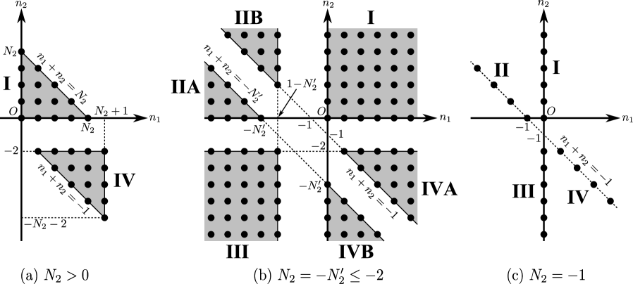
Figure 4: The regions that can contribute to $\Phi(1,N_{2})$. (a), (b): For $(n_{1},n_{2})\in{\mathbb{Z}}^{2}$ in the shaded regions (denoted by dots), the summand in $\Phi(1,N_{2})$ in (C.42) is ${\cal O}(1)$. Outside the shaded regions, the summand is ${\cal O}(\epsilon,\eta)$ and vanishes as $\epsilon,\eta\to 0$. (c): the $N_{2}=-1$ case special and the summand is non-vanishing only on the dots.

In Figure 4, we described the regions in the $(n_{1},n_{2})$ plane in which the summand appearing in $\Phi(1,N_{2})$ is non-vanishing. Figure 4(a) shows that, for $N_{2}>0$, the summand is non-vanishing in the original range of summation, $n_{1}\geq 0,n_{2}\geq 0,n_{1}+n_{2}\leq N_{2}$ (region I), as it should be. We would like to extend the range in order to eliminate the $N_{2}$ dependence and thereby analytically continue $\Phi(1,N_{2})$ to negative $N_{2}$. The requirements for the extension are

1. The range specification does not involve $N_{2}$,

2. For $N_{2}>0$, it reproduces the original result (C.40).

Clearly, there are more than one ways to extend the range satisfying these requirements. One simple way would be to take $n_{1}\geq 0,n_{2}\geq 0$ as the extended range. For $N_{2}>0$, this reduces to region I and reproduces the original result, while for $N_{2}<0$ this sums over region I in Figure 4(b). (We consider $N_{2}\leq-2$, since $N_{2}=-1$ is rather exceptional as one can see in Figure 4(c). The latter case will be discussed later.) Another possible extension is $n_{2}\geq 0$. This also reproduces the original result for $N_{2}>0$, but for $N_{2}<0$ this sums over not only regions I but also IIA and IIB.

Therefore, the way to analytically continue $\Phi(1,N_{2})$ is ambiguous and, mathematically, any such choices are good (ignoring the fact that the sum may not be convergent and is only formal). Namely, the data for discrete $N_{2}\in{\mathbb{Z}}_{>0}$ is not enough to uniquely determine the analytic continuation for all $N_{2}\in{\mathbb{C}}$. Additional input comes from the physical requirement that it reproduce the known ABJ results for $N_{2}<0$. Furthermore, for $N_{2}=-1$, ${\widehat{Z}}_{\text{lens}}(2,-1)_{k}$ is expected to be related to ${\widehat{Z}}_{\text{lens}}(1,-2)_{-k}$ by the relation (C.21).

Here we simply present the prescription which satisfies these physical requirements. The explicit checks are done in the main text where it is shown that its perturbative expansions agree with the known ABJ result and, when exact non-perturbative expressions for the ABJ matrix integral are known, it reproduces them. Moreover, the fact that the prescription reproduces the relation between ${\widehat{Z}}_{\text{lens}}(2,-1)_{k}$ and ${\widehat{Z}}_{\text{lens}}(1,-2)_{-k}$ is shown for general $N_{1}$ below.

The key observation to arrive at such a prescription is that, as we can see from Figure 4(a), the summand is non-vanishing not only in the original region I but also in region IV. The meaning of this is easier to see in the $\gamma\Psi$ representation in terms of $s_{1},s_{2}$. In Figure 5, we presented the same diagram as Figure 4 but on the $(s_{1},s_{2})$ plane.

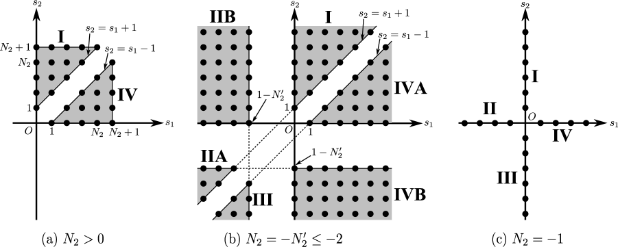
Figure 5: The regions that can contribute to $\Phi(1,N_{2})$. These are the same as Figure 4, but plotted for $(s_{1},s_{2})$ instead.

As we can see from the Figure, the non-vanishing regions have the symmetry

$$s_{1}\leftrightarrow s_{2}.$$ (C.46)

Actually, as we can immediately see from the explicit expression for $\Psi$ given in (C.44), this is a symmetry of the summand, not just its non-vanishing regions. Therefore, it is natural to relax the ordering constraint $s_{1}<s_{2}$ in the original range and sum over both regions I and IV, after dividing by $2$. If $s_{1}=s_{2}$, the summand in (C.44) automatically vanishes. Namely, we can write $\Psi$ as

$$\Psi(2,N_{2})={1\over 2}\sum_{s_{1},s_{2}=0}^{\infty}(-1)^{s_{1}+s_{2}}{(q^{s_{1}+1})_{-N_{2}-2}\over(-q^{s_{1}+1})_{-N_{2}-2}}{(q^{s_{2}+1})_{-N_{2}-2}\over(-q^{s_{2}+1})_{-N_{2}-2}}{(q^{s_{2}-s_{1}})_{1}^{2}\over(-q^{s_{2}-s_{1}})_{1}^{2}}.$$ (C.47)

Here we have extended the sum range so that $s_{1},s_{2}$ run to infinity, which is harmless in the $N_{2}>0$ case.

Our prescription is that we use the expression (C.47) even for $N_{2}=-N_{2}^{\prime}<0$. As we can see from Figure 5(b), this sums over regions I and IVA. As we have been emphasizing, it is by no means clear at this point that this is the right prescription. The justification is given in the main text where it is shown that this is consistent with all known results. One can also show that the other possible prescriptions, such as $n_{1}\geq 0,n_{2}\geq 0$, which covers region I, and $n_{2}\geq 0$, which covers regions I, IIA and IIB, would not reproduce the known results and hence are not correct.

If we set $N_{2}\to N_{2}+\epsilon$, the behavior of $\gamma$ is

$$\gamma(2,N_{2}+\epsilon)=\left({\epsilon\ln q\over 2}\right)^{2}\qquad\text{for all $N_{2}\in{\mathbb{Z}}$.}$$ (C.48)

Substituting this and (C.23) into (C.19), we finally obtain the expression for the ABJ partition function ${\widehat{Z}}_{\text{ABJ}}(2,N_{2}^{\prime})_{k}={\widehat{Z}}_{\text{lens}}(2,-N_{2}^{\prime})_{k}$:

$${\widehat{Z}}_{\text{ABJ}}(2,N_{2}^{\prime})_{k} =i^{-{\kappa\over 2}N_{2}^{\prime 2}}(2\pi)^{2+{N_{2}^{\prime 2}\over 2}}g_{s}^{1+{N_{2}^{\prime}\over 2}}(1-q)^{{1\over 2}(N_{2}^{\prime}-2)(N_{2}^{\prime}-3)}{G_{2}(N_{2}^{\prime}-1;q)\over 4G_{2}(N_{2}^{\prime}+1)}\Psi(2,-N_{2}^{\prime}),$$ (C.49)

where it is assumed that $N_{2}^{\prime}\geq 2$ and $\Psi(1,-N_{2}^{\prime})$ is given simply by setting $N_{2}=-N_{2}^{\prime}$ in (C.47):

$$\Psi(2,-N_{2}^{\prime})={1\over 2}\sum_{s_{1},s_{2}=0}^{\infty}(-1)^{s_{1}+s_{2}}{(q^{s_{1}+1})_{N_{2}^{\prime}-2}\over(-q^{s_{1}+1})_{N_{2}^{\prime}-2}}{(q^{s_{2}+1})_{N_{2}^{\prime}-2}\over(-q^{s_{2}+1})_{N_{2}^{\prime}-2}}{(q^{s_{2}-s_{1}})_{1}^{2}\over(-q^{s_{2}-s_{1}})_{1}^{2}}.$$ (C.50)

The above formula is valid for $N_{2}^{\prime}\geq 2$ but not for $N_{2}^{\prime}=1$. This case is important, because $(N_{1},N_{2}^{\prime})=(2,1)$ is related to $(N_{1},N_{2}^{\prime})=(1,2)$ by (C.21) and therefore the summation over two variables $s_{1},s_{2}$ should truncate to a sum with one variable; this provides a further check of our prescription. We will discuss this more generally below, where we discuss general $N_{1}$.

C.2.3 General $\boldsymbol{N_{1}}$

With the $N_{1}=1,2$ cases understood, the prescription for general $N_{1}$ is straightforward to establish, although computations get cumbersome. Much as in the $N_{1}=1,2$ cases, the general expression for $S$ in (B.17) can be rewritten in the following form:

$$S(N_{1},N_{2}) =\sum_{1\leq C_{1}<\cdots<C_{N_{1}}\leq N}\prod_{j=1}^{N_{1}}\Biggl{\{}\Biggl{[}\prod_{k=j}^{N_{1}-1}\prod_{a=C_{k}+1}^{C_{k+1}-1}{q^{C_{j}}+q^{a}\over q^{C_{j}}-q^{a}}\Biggr{]}\prod_{a=C_{N_{1}}+1}^{N}{q^{C_{j}}+q^{a}\over q^{C_{j}}-q^{a}}$$

$$\qquad\qquad\qquad\qquad\qquad\times\prod_{a=1}^{C_{1}-1}{q^{a}+q^{C_{j}}\over q^{a}-q^{C_{j}}}\Biggl{[}\prod_{k=1}^{j-1}\prod_{a=C_{k}+1}^{C_{k+1}-1}{q^{a}+q^{C_{j}}\over q^{a}-q^{C_{j}}}\Biggr{]}\Biggr{\}}$$

$$=\sum_{1\leq C_{1}<\cdots<C_{N_{1}}\leq N}\prod_{j=1}^{N_{1}}\Biggl{\{}\Biggl{[}\prod_{k=j}^{N_{1}-1}{(-q^{C_{k}-C_{j}+1})_{C_{k+1}-C_{k}-1}\over(q^{C_{k}-C_{j}+1})_{C_{k+1}-C_{k}-1}}\Biggr{]}{(-q^{C_{N_{1}}-C_{j}+1})_{N-C_{N_{1}}}\over(q^{C_{N_{1}}-C_{j}+1})_{N-C_{N_{1}}}}$$

$$\qquad\qquad\qquad\qquad\times{(-q^{C_{j}-C_{1}+1})_{C_{1}-1}\over(q^{C_{j}-C_{1}+1})_{C_{1}-1}}\Biggl{[}\prod_{k=1}^{j-1}{(-q^{C_{j}-C_{k+1}+1})_{C_{k+1}-C_{k}-1}\over(q^{C_{j}-C_{k+1}+1})_{C_{k+1}-C_{k}-1}}\Biggr{]}\Biggr{\}}.$$ (C.51)

In expressions such as this, it is understood that $\sum_{l=a}^{b}...=0$ and $\prod_{l=a}^{b}...=1$ if $a>b$.

Again, we can rewrite this in the $\beta\Phi$ and $\gamma\Psi$ representations. The $\beta\Phi$ representation is

$$S(N_{1},N_{2})=\beta(N_{1},N_{2})\,\Phi(N_{1},N_{2}),$$ (C.52)

$$\beta(N_{1},N_{2}):=\prod_{j=1}^{N_{1}}{(-q^{N_{1}-j+1})_{N_{2}}\over(q^{N_{1}-j+1})_{N_{2}}},$$ (C.53)

$$\Phi(N_{1},N_{2}):=\sum_{n_{1},\dots,n_{N_{1}}}(-1)^{\sum_{l=1}^{N_{1}}(N_{1}-l+1)n_{l}}$$

$$\quad\times\left[\prod_{j=1}^{N_{1}-1}\prod_{k=j}^{N_{1}-1}{(q^{k-j+1})_{n_{j+1,k}}(-q^{k-j+1})_{n_{j+1,k+1}}^{2}(q^{k-j+1})_{n_{j+2,k+1}}\over(-q^{k-j+1})_{n_{j+1,k}}(q^{k-j+1})_{n_{j+1,k+1}}^{2}(-q^{k-j+1})_{n_{j+2,k+1}}}\right]$$

$$\quad\times\left[\,\prod_{j=1}^{N_{1}}{(q^{N_{1}-j+1})_{n_{j+1,N_{1}}}(q^{-N_{1}-N_{2}+j})_{n_{1,j}}\over(-q^{N_{1}-j+1})_{n_{j+1,N_{1}}}(-q^{-N_{1}-N_{2}+j})_{n_{1,j}}}\right]\left[\prod_{k=0}^{N_{1}-1}{(-q^{k+1})_{n_{1,k+1}}(q^{k+1})_{n_{2,k+1}}\over(q^{k+1})_{n_{1,k+1}}(-q^{k+1})_{n_{2,k+1}}}\right],$$ (C.54)

where we defined $n_{1}=C_{1}-1$, $n_{j}=C_{j}-C_{j-1}-1$ ($j=2,\dots,N_{1}$), and $n_{a,b}:=\sum_{l=a}^{b}n_{l}$. Furthermore, we define $n_{N_{1}+1,b}=n_{a,N_{1}+1}=0$. The original sum range $1\leq C_{1}<\dots<C_{N_{1}}\leq N$ corresponds to $n_{j}\geq 0$ ($j=1,\dots,N_{1}$), $n_{1}+\cdots+n_{N_{1}}\leq N_{2}$, but we did not specify it in (C.54) for the same reason as in the $N_{1}=2$ case. $\Phi$ has the form of the multi-variable generalization of $q$-hypergeometric functions, discussed e.g. in [67]. When we analytically continue by $N_{2}\to-N_{2}^{\prime}+\epsilon$, $\beta(N_{1},-N_{2}^{\prime}+\epsilon)$ goes to zero, while $\Phi(N_{1},-N_{2}^{\prime})$ remains finite. The behavior of $\beta$ as $\epsilon\to 0$ is

$$\beta(N_{1},-N_{2}^{\prime}+\epsilon)=\begin{cases}\left(-{\epsilon\log q\over 2}\right)^{N_{2}^{\prime}}(-1)^{{1\over 2}N_{2}^{\prime}(N_{2}^{\prime}-1)}\prod_{j=1}^{N_{2}^{\prime}-1}{(q)_{j}\over(-q)_{j}}\prod_{j=N_{1}-N_{2}^{\prime}}^{N_{1}-1}{(q)_{j}\over(-q)_{j}}&(N_{2}^{\prime}\leq N_{1}),\\[8.61108pt] \left(-{\epsilon\log q\over 2}\right)^{N_{1}}(-1)^{N_{1}N_{2}^{\prime}+{1\over 2}N_{1}(N_{1}+1)}\prod_{j=1}^{N_{1}-1}{(q)_{j}\over(-q)_{j}}\prod_{j=N_{2}^{\prime}-N_{1}}^{N_{2}^{\prime}-1}{(q)_{j}\over(-q)_{j}}&(N_{1}\leq N_{2}^{\prime}).\end{cases}$$ (C.55)

On the other hand, the $\gamma\Psi$ representation is

$$S(N_{1},N_{2}) =\gamma(N_{1},N_{2})\,\Psi(N_{1},N_{2}),$$ (C.56)

$$\gamma(N_{1},N_{2}) =(-1)^{{1\over 2}N_{1}(N_{1}-1)}\prod_{j=1}^{N_{1}-1}{(-q)_{j}^{2}\over(q)_{j}^{2}}\prod_{j=1}^{N_{1}}{(-q^{j})_{N_{2}}(-q^{j})_{-N_{1}-N_{2}}\over(q^{j})_{N_{2}}(q^{j})_{-N_{1}-N_{2}}},$$ (C.57)

$$\Psi(N_{1},N_{2}) ={1\over N_{1}!}\sum_{s_{1},\dots,s_{N_{1}}=0}^{\infty}(-1)^{s_{1}+\cdots+s_{N_{1}}}\prod_{j=1}^{N_{1}}{(q^{s_{j}+1})_{-N_{1}-N_{2}}\over(-q^{s_{j}+1})_{-N_{1}-N_{2}}}\prod_{1\leq j<k\leq N_{1}}{(q^{s_{k}-s_{j}})_{1}^{2}\over(-q^{s_{k}-s_{j}})_{1}^{2}},$$ (C.58)

where $s_{j}:=C_{j}-1,j=1,\dots,N_{1}$. The original sum range corresponds to $0\leq s_{1}<\cdots<s_{N_{1}}\leq N-1$. However, because of the $s_{j}\leftrightarrow s_{k}$ symmetry of this expression, we can forget about the ordering constraints and let $s_{j}$ run freely, if one divides the expression by $N_{1}!$, which we have already done above. Furthermore, just as in the $N_{1}=2$ case, we can safely remove the upper bound in the summation for $N_{2}>0$. Our prescription for analytic continuation to $N_{2}<0$ is to use this same expression (C.58), by setting $N_{2}=-N_{2}^{\prime}+\epsilon$ with $\epsilon\to 0$.

The behavior of $\gamma(N_{1},N_{2})$ near integral $N_{2}$ can be shown to be

$$\gamma(N_{1},N_{2}+\epsilon)=(-1)^{N_{1}N_{2}+N_{1}}\left(-{\epsilon\ln q\over 2}\right)^{N_{1}}\qquad\text{for all $N_{2}\in{\mathbb{Z}}$.}$$ (C.59)

By substituting (C.56) and (C.23) into (C.19), we obtain the expression for the ABJ partition function ${\widehat{Z}}_{\text{ABJ}}(N_{1},N_{2}^{\prime})_{k}={\widehat{Z}}_{\text{lens}}(N_{1},-N_{2}^{\prime})_{k}$:

$${\widehat{Z}}_{\text{ABJ}}(N_{1},N_{2}^{\prime})_{k} =i^{-{\kappa\over 2}(N_{1}^{2}+N_{2}^{\prime 2})}(-1)^{{1\over 2}N_{1}(N_{1}-1)}2^{-N_{1}}(2\pi)^{N_{1}^{2}+N_{2}^{\prime 2}\over 2}g_{s}^{N_{1}+N_{2}^{\prime}\over 2}$$

$$\qquad\qquad\times(1-q)^{{1\over 2}(N_{2}^{\prime}-N_{1})(N_{2}^{\prime}-N_{1}-1)}B(N_{2}^{\prime}-N_{1},N_{1},N_{2})\Psi(N_{1},-N_{2}^{\prime})$$

$$=i^{-{\kappa\over 2}(N_{1}^{2}+N_{2}^{\prime 2})}(-1)^{{1\over 2}N_{1}(N_{1}-1)}2^{-N_{1}}(2\pi)^{N_{1}^{2}+N_{2}^{\prime 2}\over 2}g_{s}^{N_{1}+N_{2}^{\prime}\over 2}$$

$$\qquad\qquad\qquad\times{\prod_{j=1}^{N_{2}^{\prime}-N_{1}-1}(q)_{j}\over G_{2}(N_{1}+1)G_{2}(N_{2}^{\prime}+1)}\Psi(N_{1},-N_{2}^{\prime}),$$ (C.60)

where we assumed that $N_{2}^{\prime}\geq N_{1}$ and

$$\Psi(N_{1},-N_{2}^{\prime})={1\over N_{1}!}\sum_{s_{1},\dots,s_{N_{1}}=0}^{\infty}(-1)^{s_{1}+\cdots+s_{N_{1}}}\prod_{j=1}^{N_{1}}{(q^{s_{j}+1})_{N_{2}^{\prime}-N_{1}}\over(-q^{s_{j}+1})_{N_{2}^{\prime}-N_{1}}}\prod_{1\leq j<k\leq N_{1}}{(1-q^{s_{k}-s_{j}})^{2}\over(1+q^{s_{k}-s_{j}})^{2}}.$$ (C.61)

The above expression is valid only for $N_{2}^{\prime}\geq N_{1}$. If $N_{2}^{\prime}<N_{1}$, then the summation in (C.61) over $N_{1}$ variables should reduce to that of ${\widehat{Z}}_{\text{lens}}(N_{2}^{\prime},-N_{1})_{k}$ over $N_{2}^{\prime}$ variables to be consistent with the symmetry (C.21). Let us see how this works by setting $N_{2}^{\prime}\to N_{2}^{\prime}-\epsilon$ in (C.61). Because of (C.23) and (C.59), only terms that diverge as $\sim\epsilon^{-(N_{1}-N_{2}^{\prime})}$ in the $s$-sum survive. Divergences can appear from

$$(q^{s_{j}+1})_{N_{2}^{\prime}-N_{1}-\epsilon}={1\over(q^{s_{j}+1+N_{2}^{\prime}-N_{1}-\epsilon})_{N_{1}-N_{2}^{\prime}}}={1\over(1-q^{s_{j}+1+N_{2}^{\prime}-N_{1}-\epsilon})\cdots(1-q^{s_{j}-\epsilon})},$$ (C.62)

where we are keeping only the leading term. For this to give a divergent $(\sim\epsilon^{-1})$ contribution, it should be that $s_{j}+1+N_{2}^{\prime}-N_{1}\leq 0$, namely, $s_{j}\leq N_{1}-N_{2}^{\prime}-1$ (this is impossible for $N_{1}\leq N_{2}^{\prime}$). Because $s_{1},\dots,s_{N_{1}}$ should be different from one another, the most singular case we can have is when $\{s_{1},\dots,s_{N_{1}}\}\supset\{0,1,\dots,N_{1}-N_{2}^{\prime}-1\}$. In this case, we have precisely ${\cal O}(\epsilon^{-(N_{1}-N_{2}^{\prime})})$. Concretely, let us set

$$s_{j} =\begin{cases}j-1&\quad(1\leq j\leq N_{1}-N_{2}^{\prime}),\\ N_{1}-N_{2}^{\prime}+s^{\prime}_{j-N_{1}+N_{2}^{\prime}}&\quad(N_{1}-N_{2}^{\prime}+1\leq j\leq N_{2}^{\prime})\end{cases}$$ (C.63)

with $s_{j}^{\prime}\geq 0$ and multiply the result by a combinatoric factor ${N_{1}\choose N_{1}-N_{2}^{\prime}}\cdot(N_{1}-N_{2}^{\prime})!={N_{1}!\over N_{2}^{\prime}!}$. By substituting these into (C.61) and massaging the result, we can show

$$\Psi(N_{1},-N_{2}^{\prime}+\epsilon)=(-1)^{N_{1}N_{2}^{\prime}+N_{1}}\left(-{2\over\epsilon\ln q}\right)^{N_{1}-N_{2}^{\prime}}$$ (C.64)

$$\qquad\times{1\over N_{2}^{\prime}!}\sum_{s_{1}^{\prime},\dots,s_{N_{2}^{\prime}}^{\prime}=0}^{\infty}\!\!(-1)^{s_{1}^{\prime}+\cdots+s_{N_{2}^{\prime}}^{\prime}}\prod_{j=1}^{N_{2}^{\prime}}{(q^{s_{j}^{\prime}+1})_{N_{1}-N_{2}^{\prime}}\over(-q^{s_{j}^{\prime}+1})_{N_{1}-N_{2}^{\prime}}}\prod_{1\leq j<k\leq N_{2}^{\prime}}{(q^{s_{k}^{\prime}-s_{j}^{\prime}})_{1}^{2}\over(-q^{s_{k}^{\prime}-s_{j}^{\prime}})_{1}^{2}}\qquad(N_{2}^{\prime}\leq N_{1}).$$

Namely, the summation over $N_{1}$ variables $s_{1},\dots,s_{N_{1}}$ correctly reduced to summation over $N_{2}^{\prime}$ variables $s^{\prime}_{1},\dots,s^{\prime}_{N_{2}^{\prime}}$, and the $\epsilon$ dependence of $\Psi$, combined with $\gamma\sim\epsilon^{N_{1}}$, is the correct one to cancel the divergence of $B\sim\epsilon^{-N_{2}^{\prime}}$ (see (C.23)). So, for $N_{2}^{\prime}<N_{1}$, the expression for the ABJ partition function ${\widehat{Z}}_{\text{ABJ}}(N_{1},N_{2}^{\prime})_{k}={\widehat{Z}}_{\text{lens}}(N_{1},-N_{2}^{\prime})_{k}$ is

$${\widehat{Z}}_{\text{lens}}(N_{1},-N_{2}^{\prime})_{k} =i^{-{\kappa\over 2}(N_{1}^{2}+N_{2}^{\prime 2})}(-1)^{{1\over 2}N_{2}^{\prime}(N_{2}^{\prime}-1)}2^{-N_{2}^{\prime}}(2\pi)^{N_{1}^{2}+N_{2}^{\prime 2}\over 2}g_{s}^{N_{1}+N_{2}^{\prime}\over 2}q^{-{1\over 6}(N_{1}-N_{2}^{\prime})((N_{1}-N_{2}^{\prime})^{2}-1)}$$

$$\qquad\qquad\times(1-q)^{{1\over 2}(N_{1}-N_{2}^{\prime})(N_{1}-N_{2}^{\prime}-1)}B(N_{1}-N_{2}^{\prime},N_{1},N_{2}^{\prime})\Psi(N_{2}^{\prime},-N_{1})$$

$$=i^{-{\kappa\over 2}(N_{1}^{2}+N_{2}^{\prime 2})}(-1)^{{1\over 2}N_{2}^{\prime}(N_{2}^{\prime}-1)}2^{-N_{2}^{\prime}}(2\pi)^{N_{1}^{2}+N_{2}^{\prime 2}\over 2}g_{s}^{N_{1}+N_{2}^{\prime}\over 2}$$

$$\qquad\qquad\times{q^{-{1\over 6}(N_{1}-N_{2}^{\prime})((N_{1}-N_{2}^{\prime})^{2}-1)}\prod_{j=1}^{N_{1}-N_{2}^{\prime}-1}(q)_{j}\over G_{2}(N_{1}+1)G_{2}(N_{2}^{\prime}+1)}\Psi(N_{2}^{\prime},-N_{1}),$$ (C.65)

where

$$\Psi(N_{2}^{\prime},-N_{1})={1\over N_{2}^{\prime}!}\sum_{s_{1}^{\prime},\dots,s_{N_{2}^{\prime}}^{\prime}=0}^{\infty}\!\!(-1)^{s_{1}^{\prime}+\cdots+s_{N_{2}^{\prime}}^{\prime}}\prod_{j=1}^{N_{2}^{\prime}}{(q^{s_{j}^{\prime}+1})_{N_{1}-N_{2}^{\prime}}\over(-q^{s_{j}^{\prime}+1})_{N_{1}-N_{2}^{\prime}}}\prod_{1\leq j<k\leq N_{2}^{\prime}}{(q^{s_{k}^{\prime}-s_{j}^{\prime}})_{1}^{2}\over(-q^{s_{k}^{\prime}-s_{j}^{\prime}})_{1}^{2}}\qquad(N_{2}^{\prime}\leq N_{1}).$$ (C.66)

Using the explicit expressions (C.60) and (C.65), It is straightforward to show that the relation (C.21) between ${\widehat{Z}}_{\text{lens}}(N_{1},-N_{2}^{\prime})_{k}$ and ${\widehat{Z}}_{\text{lens}}(N_{2}^{\prime},-N_{1})_{-k}$ holds.

In Table 2, we present a summary of how various quantities behave as $\epsilon\to 0$ for various values of $N_{2}$.

range of $N_{2}$	$B$	$\beta$	$\Phi$	$\gamma$	$\Psi$	$S=\beta\Phi=\gamma\Psi$	${\widehat{Z}}\propto BS$
$N_{2}>0$	finite	finite	finite	$\epsilon^{N_{1}}$	$\epsilon^{-N_{1}}$	finite	finite
$N_{2}<0$,  $0<N_{2}^{\prime}\leq N_{1}$	$\epsilon^{-N_{2}^{\prime}}$	$\epsilon^{N_{2}^{\prime}}$	finite	$\epsilon^{N_{1}}$	$\epsilon^{N_{2}^{\prime}-N_{1}}$	$\epsilon^{N_{2}^{\prime}}$	finite
$N_{2}<0$,  $N_{1}\leq N_{2}^{\prime}$	$\epsilon^{-N_{1}}$	$\epsilon^{N_{1}}$	finite	$\epsilon^{N_{1}}$	finite	$\epsilon^{N_{1}}$	finite

Table 2: The $\epsilon\to 0$ behavior of various quantities for general $N_{1}$. If $N_{2}<0$, we define $N_{2}^{\prime}=-N_{2}$.

Appendix D The perturbative free energy

In this appendix, we present the free energy of the lens space matrix model computed by perturbative expansion, up to eight loop order ${\cal O}(g_{s}^{8})$:

$$F_{\rm lens}(N_{1},N_{2})-F^{\rm tree}_{\rm lens}(N_{1},N_{2})=g_{s}\biggl{(}\frac{N_{1}^{3}}{12}+\frac{N_{1}^{2}N_{2}}{4}+\frac{N_{1}N_{2}^{2}}{4}+\frac{N_{2}^{3}}{12}-\frac{N_{1}}{12}-\frac{N_{2}}{12}\biggr{)}\\ +g_{s}^{2}\left(\frac{N_{1}^{4}}{288}+\frac{N_{1}^{3}N_{2}}{48}+\frac{N_{2}^{2}N_{1}^{2}}{16}+\frac{N_{2}^{3}N_{1}}{48}+\frac{N_{2}^{4}}{288}-\frac{N_{1}^{2}}{288}+\frac{N_{1}N_{2}}{48}-\frac{N_{2}^{2}}{288}\right)\\ +g_{s}^{4}\biggl{(}-\frac{N_{1}^{6}}{86400}-\frac{N_{1}^{5}N_{2}}{7680}-\frac{N_{1}^{4}N_{2}^{2}}{1536}-\frac{5N_{1}^{3}N_{2}^{3}}{1152}-\frac{N_{1}^{2}N_{2}^{4}}{1536}-\frac{N_{1}N_{2}^{5}}{7680}-\frac{N_{2}^{6}}{86400}\\ +\frac{N_{1}^{4}}{34560}+\frac{7N_{1}^{3}N_{2}}{4608}-\frac{N_{1}^{2}N_{2}^{2}}{768}+\frac{7N_{1}N_{2}^{3}}{4608}+\frac{N_{2}^{4}}{34560}-\frac{N_{1}^{2}}{57600}-\frac{N_{1}N_{2}}{960}-\frac{N_{2}^{2}}{57600}\biggr{)}\\ +g_{s}^{6}\biggl{(}\frac{N_{1}^{8}}{10160640}+\frac{N_{1}^{7}N_{2}}{645120}+\frac{N_{1}^{6}N_{2}^{2}}{92160}+\frac{N_{1}^{5}N_{2}^{3}}{92160}+\frac{7N_{1}^{4}N_{2}^{4}}{9216}+\frac{N_{1}^{3}N_{2}^{5}}{92160}+\frac{N_{1}^{2}N_{2}^{6}}{92160}+\frac{N_{1}N_{2}^{7}}{645120}+\frac{N_{2}^{8}}{10160640}\\ -\frac{N_{1}^{6}}{2177280}+\frac{N_{1}^{5}N_{2}}{92160}-\frac{N_{1}^{4}N_{2}^{2}}{2304}+\frac{N_{1}^{3}N_{2}^{3}}{27648}-\frac{N_{1}^{2}N_{2}^{4}}{2304}+\frac{N_{1}N_{2}^{5}}{92160}-\frac{N_{2}^{6}}{2177280}\\ +\frac{N_{1}^{4}}{1451520}+\frac{N_{1}^{3}N_{2}}{11520}+\frac{N_{1}^{2}N_{2}^{2}}{3840}+\frac{N_{1}N_{2}^{3}}{11520}+\frac{N_{2}^{4}}{1451520}-\frac{N_{1}^{2}}{3048192}-\frac{N_{1}N_{2}}{12096}-\frac{N_{2}^{2}}{3048192}\biggr{)}\\ +g_{s}^{8}\biggl{(}-\frac{N_{1}^{10}}{870912000}-\frac{17N_{1}^{9}N_{2}}{743178240}-\frac{17N_{1}^{8}N_{2}^{2}}{82575360}-\frac{N_{1}^{7}N_{2}^{3}}{774144}+\frac{97N_{1}^{6}N_{2}^{4}}{4423680}-\frac{2821N_{1}^{5}N_{2}^{5}}{14745600}+\frac{97N_{1}^{4}N_{2}^{6}}{4423680}\\ -\frac{N_{1}^{3}N_{2}^{7}}{774144}-\frac{17N_{1}^{2}N_{2}^{8}}{82575360}-\frac{17N_{1}N_{2}^{9}}{743178240}-\frac{N_{2}^{10}}{870912000}+\frac{N_{1}^{8}}{116121600}+\frac{29N_{1}^{7}N_{2}}{123863040}-\frac{259N_{1}^{6}N_{2}^{2}}{17694720}\\ +\frac{937N_{1}^{5}N_{2}^{3}}{8847360}+\frac{53N_{1}^{4}N_{2}^{4}}{442368}+\frac{937N_{1}^{3}N_{2}^{5}}{8847360}-\frac{259N_{1}^{2}N_{2}^{6}}{17694720}+\frac{29N_{1}N_{2}^{7}}{123863040}+\frac{N_{2}^{8}}{116121600}-\frac{N_{1}^{6}}{41472000}\\ +\frac{853N_{1}^{5}N_{2}}{58982400}-\frac{1487N_{1}^{4}N_{2}^{2}}{11796480}-\frac{83N_{2}^{3}N_{1}^{3}}{1769472}-\frac{1487N_{1}^{2}N_{2}^{4}}{11796480}+\frac{853N_{1}N_{2}^{5}}{58982400}-\frac{N_{2}^{6}}{41472000}+\frac{N_{1}^{4}}{34836480}\\ -\frac{23N_{1}^{3}N_{2}}{37158912}+\frac{325N_{1}^{2}N_{2}^{2}}{3096576}-\frac{23N_{1}N_{2}^{3}}{37158912}+\frac{N_{2}^{4}}{34836480}-\frac{N_{1}^{2}}{82944000}-\frac{17N_{1}N_{2}}{1382400}-\frac{N_{2}^{2}}{82944000}\biggr{)}\ .$$ (D.1)

This perfectly agrees with the result in [37] to the order presented there. Meanwhile, we have explicitly checked that the perturbative free energy of the ABJ matrix model is indeed related to the lens space free energy by

$$F_{\rm ABJ}(N_{1},N_{2})=F_{\rm lens}(N_{1},-N_{2})\ ,$$ (D.2)

including the tree contribution with the normalization discussed in Appendix C.1.

Appendix E The Seiberg duality

In this Appendix, we show that the $(1,N_{1})$ ABJ partition function $Z_{\rm ABJ}(1,N_{1})_{k}$ given in (4.8) is invariant under the Seiberg duality (4.7) up to a phase. Because in the main text we have shown that $Z_{\rm CS}^{0}(N_{2}-1)_{k}$ is invariant and that the phase factor precisely agrees with the one given in [56], all that remains to be shown is the invariance of the integral $I(1,N_{2})_{k}$ defined in (4.10).

As claimed in the main text, for Seiberg dual pairs, we can show that the integrand appearing in $I(1,N_{2})_{k}$ is the same up to a shift in $s$. More precisely, the claim to be proven is that the integrand

$$f_{N_{2}}(s):={\pi\over\sin(\pi s)}\prod_{j=1}^{N_{2}-1}\tan{\pi(s+j)\over|k|}$$ (E.1)

has the following property:

$$f_{N_{2}}(s)=f_{{\widetilde{N}}_{2}}\!\!\left(s-{|k|\over 2}+N_{2}-1\right),\qquad{\widetilde{N}}_{2}:=2+|k|-N_{2}.$$ (E.2)

Therefore, as long as we take the prescription (4.13) for the contour, $I(1,N_{2})_{k}$ defined by the contour integral (4.10) remains the same.

Note that, if two meromorphic functions $f(s)$ and $g(s)$ have poles and zeros at the same points and with the same order, then they must be equal to each other up to an overall constant. This can be shown as follows. If $z=\alpha$ is a pole or a zero, we can write $f(s)=a(z-\alpha)^{n},g(s)=b(z-\alpha)^{n}$ near $z=\alpha$ by the assumption. This means that $f^{\prime}/f=g^{\prime}/g=n(z-\alpha)^{-1}$ near $z=\alpha$. Now, recall that Mittag-Leffler’s theorem in complex analysis states that, if two functions have poles at the same points and if the singular part of the Laurent expansion around each of them is the same, then the two functions are identical. So, because $f^{\prime}/f$ and $g^{\prime}/g$ share poles and residues, they must be identical. This means that $f(s)=cg(s)$ with a constant $c$. In the present case, it is easy to show that the overall scale of $f_{N_{2}}(s)$ and $f_{{\widetilde{N}}_{2}}(s-{|k|\over 2}+N_{2}-1)$ is the same asymptotically, because both tend to ${2\pi i^{N_{2}-2}e^{-\pi\sigma}}$ for $s=i\sigma$, $\sigma\to+\infty$. So, in order to show that these two functions are equal, we only have to show that they share poles and zeros.

So, let us compare the poles and zeros of the two functions $f_{N_{2}}(s)$ and $f_{{\widetilde{N}}_{2}}(s-{|k|\over 2}+N_{2}-1)$. Recall the expression for $f_{N_{2}}(s)$ given by (E.1). First, ${\pi\over\sin(\pi s)}$ gives simple poles at $s\in{\mathbb{Z}}$ (P poles) but no zero. On the other hand, $\tan{\pi(s+j)\over|k|}$ gives simple poles at $s=|k|(p+{1\over 2})-j$, $p\in{\mathbb{Z}}$ (NP poles), and simple zeros at $s=|k|q-j$, $q\in{\mathbb{Z}}$ (NP zeros). Using this data, we can find the pole/zero structure of the two functions as we discuss now. We should consider odd and even $k$ cases separately,

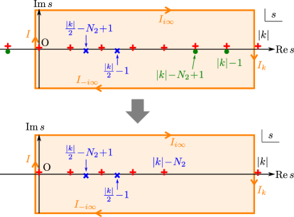
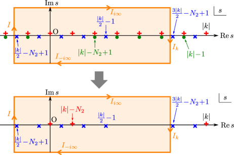
(a) ${|k|\over 2}-N_{2}+1\geq 1$ (shown is the $N_{2}=3,|k|=7$ case).	(b) ${|k|\over 2}-N_{2}+1\leq 1$ (shown is the $N_{2}=6,|k|=7$ case).

Figure 6: The pole/zero structure of the integrand function for odd $k$. “$+$” (red) denotes the P pole, “$\times$” (blue) the NP pole, and “$\bullet$” (green) the NP zero. Some poles and zeros are shown slightly above or below the real $s$ axis, but this is for the convenience of presentation and all poles and zeros are on the real $s$ axis. If the original theory is in case (a) ${|k|\over 2}-N_{2}+1\geq 1$, then the Seiberg dual is in case (b) ${|k|\over 2}-N_{2}+1\leq 1$, and vice versa. In the figure, actual Seiberg dual theories are shown. In the upper panels, all P poles coming from ${\pi\over\sin\pi s}$ and all NP poles and NP zeros coming from $\prod_{j}\tan$ are shown. In the lower panels, P poles and NP zeros that cancel each other are removed. We see that the actual poles are the same in the dual theories (a) and (b), with P and NP poles interchanged.

Odd $\boldsymbol{k}$:

For odd $k$, $f_{N_{2}}(s)$ has poles but no zeros. All poles are simple poles and they can be divided into two groups:

$$\begin{split}\rm P&:\qquad s=0,\dots,|k|-N_{2},\\ \rm NP&:\qquad s={|k|\over 2}-N_{2}+1,\dots,{|k|\over 2}-1,\end{split}$$ (E.3)

where periodicity $s\cong s+|k|$ is understood; see Figure 6. Note that this is valid even for ${|k|\over 2}-N_{2}+1<0$, for which some of the poles are at $s<0$. P means poles coming from $\pi\over\sin\pi s$ while NP means poles coming from $\prod_{j}\tan$. Some of the P poles got canceled by NP zeros and reduced to regular points. NP poles are not canceled. P and NP poles never collide, because the former are at integral $s$ while the latter are at half-odd-integral $s$.

(E.3) means that $f_{{\widetilde{N}}_{2}}(s)$ has simple poles at

$$\begin{split}\rm P&:\qquad s=0,\dots,|k|-{\widetilde{N}}_{2}=0,\dots,-2+N_{2},\\ \rm NP&:\qquad s={|k|\over 2}-N_{2}+1,\dots,{|k|\over 2}-1=-{|k|\over 2}+N_{2}-1,\dots,{|k|\over 2}-1,\end{split}$$ (E.4)

which in turn means that $f_{{\widetilde{N}}_{2}}(s+N_{2}-{|k|\over 2}-1)$ has simple poles at

$$\begin{split}\rm P&:\qquad s={|k|\over 2}-N_{2}+1,\dots,{|k|\over 2}-1,\\ \rm NP&:\qquad s=0,\dots,|k|-N_{2};\end{split}$$ (E.5)

This is the same as (E.3), with P and NP interchanged. This proves the identity (E.2) for odd $k$. Figure 6 shows the explicit pole/zero structure in the specific case of $U(1)_{7}\times U(3)_{-7}=U(1)_{-7}\times U(6)_{7}$.

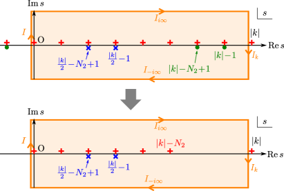
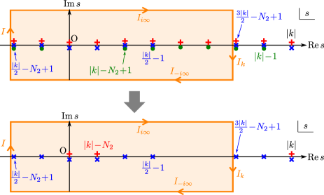
(a) ${|k|\over 2}-N_{2}+1\geq 1$ (shown is the $N_{2}=3,|k|=8$ case).	(b) ${|k|\over 2}-N_{2}+1\leq 1$ (shown is the $N_{2}=7,|k|=8$ case).

Figure 7: The pole/zero structure of the integrand function for even $k$. See Figure 6 for explanation of the symbols. In the figure, actual Seiberg dual theories are shown. In the upper panels, all P poles coming from ${\pi\over\sin\pi s}$ and all NP poles and NP zeros coming from $\prod_{j}\tan$ are shown. In the lower panels, poles that are canceled by NP zeros are removed. If a P pole, a NP pole and a NP zero all collide, the resulting simple pole is interpreted as a NP pole. The surviving poles are the same in the dual theories (a) and (b), with P and NP poles interchanged.

Even $\boldsymbol{k}$:

Also for even $k$, the function $f_{N_{2}}(s)$ has poles but no zeros. Some of the poles are simple while others are double. Let us think of a double pole as made of two simple poles on top of each other. Then there are two groups of simple poles, as follows:

$$\begin{split}\rm P&:\qquad s=0,\dots,|k|-N_{2},\\ \rm NP&:\qquad s={|k|\over 2}-N_{2}+1,\dots,{|k|\over 2}-1,\end{split}$$ (E.6)

where $s\cong s+|k|$ is again implied; see Figure 7. For $k$ even, NP zeros can cancel P poles and NP poles, and it becomes ambiguous whether we should call a particular pole P or NP. This happens in the ${|k|\over 2}-N_{2}+1<0$ case, where a P pole, a NP pole and a NP zero all can be at the same point. When this happens, we think of the P pole getting canceled by the NP zero, and group the remaining simple pole into NP, as we did above. This is arbitrary, but it is a unique choice for which the structure (E.6) becomes identical to the odd $k$ case, (E.3).

Because (E.6) is the same as the odd $k$ case, (E.3), the rest goes exactly the same, and we conclude that $f_{N_{2}}(s)$ and $f_{{\widetilde{N}}_{2}}(s+N_{2}-{|k|\over 2}-1)$ are identical, with P and NP interchanged. Figure 7 shows the explicit pole/zero structure in the specific case of $U(1)_{8}\times U(3)_{-8}=U(1)_{-8}\times U(7)_{8}$.

References

- [1] E. Witten, “Topological Quantum Field Theory,” Commun. Math. Phys. 117, 353 (1988).
- [2] N. A. Nekrasov, “Seiberg-Witten prepotential from instanton counting,” Adv. Theor. Math. Phys. 7, 831 (2004) [hep-th/0206161].
- [3] V. Pestun, “Localization of gauge theory on a four-sphere and supersymmetric Wilson loops,” Commun. Math. Phys. 313, 71 (2012) [arXiv:0712.2824 [hep-th]].
- [4] J. K. Erickson, G. W. Semenoff and K. Zarembo, “Wilson loops in N=4 supersymmetric Yang-Mills theory,” Nucl. Phys. B 582, 155 (2000) [arXiv:hep-th/0003055].
- [5] N. Drukker and D. J. Gross, “An Exact prediction of N=4 SYM theory for string theory,” J. Math. Phys. 42, 2896 (2001) [arXiv:hep-th/0010274].
- [6] A. Kapustin, B. Willett and I. Yaakov, “Exact Results for Wilson Loops in Superconformal Chern-Simons Theories with Matter,” JHEP 1003, 089 (2010) [arXiv:0909.4559 [hep-th]];
- [7] N. Hama, K. Hosomichi and S. Lee, “SUSY Gauge Theories on Squashed Three-Spheres,” JHEP 1105, 014 (2011) [arXiv:1102.4716 [hep-th]].
- [8] O. Aharony, O. Bergman, D. L. Jafferis and J. Maldacena, “N=6 superconformal Chern-Simons-matter theories, M2-branes and their gravity duals,” JHEP 0810, 091 (2008) [arXiv:0806.1218 [hep-th]].
- [9] O. Aharony, O. Bergman and D. L. Jafferis, “Fractional M2-branes,” JHEP 0811, 043 (2008) [arXiv:0807.4924 [hep-th]].
- [10] K. Hosomichi, R. -K. Seong and S. Terashima, “Supersymmetric Gauge Theories on the Five-Sphere,” Nucl. Phys. B 865, 376 (2012) [arXiv:1203.0371 [hep-th]].
- [11] J. Kallen, J. Qiu and M. Zabzine, “The perturbative partition function of supersymmetric 5D Yang-Mills theory with matter on the five-sphere,” JHEP 1208, 157 (2012) [arXiv:1206.6008 [hep-th]].
- [12] H. -C. Kim and S. Kim, “M5-branes from gauge theories on the 5-sphere,” arXiv:1206.6339 [hep-th].
- [13] J. M. Maldacena, “The large N limit of superconformal field theories and supergravity,” Adv. Theor. Math. Phys. 2, 231 (1998) [Int. J. Theor. Phys. 38, 1113 (1999)] [arXiv:hep-th/9711200];
- [14] N. Drukker, M. Marino and P. Putrov, “From weak to strong coupling in ABJM theory,” Commun. Math. Phys. 306, 511 (2011) [arXiv:1007.3837 [hep-th]].
- [15] M. Marino, “Lectures on localization and matrix models in supersymmetric Chern-Simons-matter theories,” J. Phys. A A 44, 463001 (2011) [arXiv:1104.0783 [hep-th]].
- [16] C. P. Herzog, I. R. Klebanov, S. S. Pufu and T. Tesileanu, “Multi-Matrix Models and Tri-Sasaki Einstein Spaces,” Phys. Rev. D 83, 046001 (2011) [arXiv:1011.5487 [hep-th]].
- [17] D. L. Jafferis and S. S. Pufu, “Exact results for five-dimensional superconformal field theories with gravity duals,” arXiv:1207.4359 [hep-th].
- [18] A. Brandhuber and Y. Oz, “The D-4 - D-8 brane system and five-dimensional fixed points,” Phys. Lett. B 460, 307 (1999) [hep-th/9905148]; O. Bergman and D. Rodriguez-Gomez, “5d quivers and their AdS(6) duals,” JHEP 1207, 171 (2012) [arXiv:1206.3503 [hep-th]].
- [19] J. Kallen, J. A. Minahan, A. Nedelin and M. Zabzine, “-behavior from 5D Yang-Mills theory,” JHEP 1210, 184 (2012) [arXiv:1207.3763 [hep-th]].
- [20] M. R. Douglas, “On D=5 super Yang-Mills theory and (2,0) theory,” JHEP 1102, 011 (2011) [arXiv:1012.2880 [hep-th]]. N. Lambert, C. Papageorgakis and M. Schmidt-Sommerfeld, “M5-Branes, D4-Branes and Quantum 5D super-Yang-Mills,” JHEP 1101, 083 (2011) [arXiv:1012.2882 [hep-th]].
- [21] N. Beisert, C. Ahn, L. F. Alday, Z. Bajnok, J. M. Drummond, L. Freyhult, N. Gromov, R. A. Janik, V. Kazakov, T. Klose, G. P. Korchemsky, C. Kristjansen, M. Magro, T. McLoughlin, J. A. Minahan, R. I. Nepomechie, A. Rej, R. Roiban, S. Schafer-Nameki, C. Sieg, M. Staudacher, A. Torrielli, A. A. Tseytlin, P. Vieira, D. Volin, K. Zoubos, “Review of AdS/CFT Integrability: An Overview,” [arXiv:1012.3982 [hep-th]].
- [22] C. -M. Chang, S. Minwalla, T. Sharma and X. Yin, “ABJ Triality: from Higher Spin Fields to Strings,” arXiv:1207.4485 [hep-th].
- [23] O. Bergman, S. Hirano, “Anomalous Radius Shift in AdS4/CFT3,” JHEP 0907, 016 (2009). [arXiv:0902.1743 [hep-th]].
- [24] O. Aharony, A. Hashimoto, S. Hirano and P. Ouyang, “D-brane Charges in Gravitational Duals of 2+1 Dimensional Gauge Theories and Duality Cascades,” JHEP 1001, 072 (2010) [arXiv:0906.2390 [hep-th]].
- [25] M. Bershadsky, S. Cecotti, H. Ooguri and C. Vafa, “Kodaira-Spencer theory of gravity and exact results for quantum string amplitudes,” Commun. Math. Phys. 165, 311 (1994) [arXiv:hep-th/9309140].
- [26] N. Drukker, M. Marino and P. Putrov, “Nonperturbative aspects of ABJM theory,” JHEP 1111, 141 (2011) [arXiv:1103.4844 [hep-th]].
- [27] H. Fuji, S. Hirano and S. Moriyama, “Summing Up All Genus Free Energy of ABJM Matrix Model,” JHEP 1108, 001 (2011) [arXiv:1106.4631 [hep-th]].
- [28] S. Bhattacharyya, A. Grassi, M. Marino and A. Sen, “A One-Loop Test of Quantum Supergravity,” arXiv:1210.6057 [hep-th].
- [29] M. Marino and P. Putrov, “ABJM theory as a Fermi gas,” J. Stat. Mech. 1203, P03001 (2012) [arXiv:1110.4066 [hep-th]].
- [30] M. Marino and P. Putrov, “Interacting fermions and N=2 Chern-Simons-matter theories,” arXiv:1206.6346 [hep-th].
- [31] M. Hanada, M. Honda, Y. Honma, J. Nishimura, S. Shiba and Y. Yoshida, “Numerical studies of the ABJM theory for arbitrary N at arbitrary coupling constant,” JHEP 1205, 121 (2012) [arXiv:1202.5300 [hep-th]]. “Monte Carlo studies of 3d N=6 SCFT via localization method,” arXiv:1211.6844 [hep-lat].
- [32] A. Klemm, M. Marino, M. Schiereck and M. Soroush, “ABJM Wilson loops in the Fermi gas approach,” arXiv:1207.0611 [hep-th].
- [33] K. Okuyama, “A Note on the Partition Function of ABJM theory on ,” Prog. Theor. Phys. 127, 229 (2012) [arXiv:1110.3555 [hep-th]].
- [34] Y. Hatsuda, S. Moriyama and K. Okuyama, “Exact Results on the ABJM Fermi Gas,” JHEP 1210, 020 (2012) [arXiv:1207.4283 [hep-th]]; “Instanton Effects in ABJM Theory from Fermi Gas Approach,” arXiv:1211.1251 [hep-th].
- [35] P. Putrov and M. Yamazaki, “Exact ABJM Partition Function from TBA,” Mod. Phys. Lett. A 27, 1250200 (2012) [arXiv:1207.5066 [hep-th]].
- [36] M. Marino, “Chern-Simons theory, matrix integrals, and perturbative three manifold invariants,” Commun. Math. Phys. 253, 25 (2004) [arXiv:hep-th/0207096].
- [37] M. Aganagic, A. Klemm, M. Marino and C. Vafa, “Matrix model as a mirror of Chern-Simons theory,” JHEP 0402, 010 (2004) [hep-th/0211098].
- [38] M. Marino, P. Putrov, “Exact Results in ABJM Theory from Topological Strings,” JHEP 1006, 011 (2010). [arXiv:0912.3074 [hep-th]].
- [39] A. Kapustin, B. Willett and I. Yaakov, “Nonperturbative Tests of Three-Dimensional Dualities,” JHEP 1010, 013 (2010) [arXiv:1003.5694 [hep-th]].
- [40] O. Bergman, A. Hanany, A. Karch and B. Kol, “Branes and supersymmetry breaking in three-dimensional gauge theories,” JHEP 9910, 036 (1999) [hep-th/9908075].
- [41] A. Hashimoto, S. Hirano and P. Ouyang, “Branes and fluxes in special holonomy manifolds and cascading field theories,” JHEP 1106, 101 (2011) [arXiv:1004.0903 [hep-th]].
- [42] M. Marino, “Chern-Simons theory and topological strings,” Rev. Mod. Phys. 77, 675 (2005) [hep-th/0406005]; “Chern-Simons theory, matrix integrals, and perturbative three manifold invariants,” Commun. Math. Phys. 253, 25 (2004) [hep-th/0207096].
- [43] M. Tierz, “Soft matrix models and Chern-Simons partition functions,” Mod. Phys. Lett. A 19, 1365 (2004) [hep-th/0212128].
- [44] G. Gasper and M. Rahman, “Basic Hypergeometric Series”, 2nd edition, Cambridge, 2004.
- [45] R. Koekoek and R. F. Swarttouw, “The Askey-scheme of Hypergeometric Orthogonal Polynomials and its -analogue”, Reports of the faculty of Technical Mathematics and Informatics, No. 98-17, Delft.
- [46] H. Rosengren, “Schur Q-polynomials, multiple hypergeometric series and enumeration of marked shifted tableaux,” J. Combin. Theory A 115, 376-406 (2008) [arXiv:math/0603086 [math.CO]].
- [47] S. Giombi, S. Minwalla, S. Prakash, S. P. Trivedi, S. R. Wadia and X. Yin, “Chern-Simons Theory with Vector Fermion Matter,” Eur. Phys. J. C 72, 2112 (2012) [arXiv:1110.4386 [hep-th]].
- [48] H. Awata, S. Hirano, K. Nii and M. Shigemori, work in progress.
- [49] B. Sundborg, “Stringy gravity, interacting tensionless strings and massless higher spins,” Nucl. Phys. Proc. Suppl. 102, 113 (2001) [hep-th/0103247].
- [50] E. Sezgin and P. Sundell, “Massless higher spins and holography,” Nucl. Phys. B 644, 303 (2002) [Erratum-ibid. B 660, 403 (2003)] [hep-th/0205131].
- [51] I. R. Klebanov and A. M. Polyakov, “AdS dual of the critical O(N) vector model,” Phys. Lett. B 550, 213 (2002) [hep-th/0210114].
- [52] O. Aharony, G. Gur-Ari and R. Yacoby, “d=3 Bosonic Vector Models Coupled to Chern-Simons Gauge Theories,” JHEP 1203, 037 (2012) [arXiv:1110.4382 [hep-th]].
- [53] R. Gopakumar and C. Vafa, “On the gauge theory / geometry correspondence,” Adv. Theor. Math. Phys. 3, 1415 (1999) [hep-th/9811131].
- [54] A. Giveon and D. Kutasov, “Seiberg Duality in Chern-Simons Theory,” Nucl. Phys. B 812, 1 (2009) [arXiv:0808.0360 [hep-th]].
- [55] V. Niarchos, “Seiberg Duality in Chern-Simons Theories with Fundamental and Adjoint Matter,” JHEP 0811, 001 (2008) [arXiv:0808.2771 [hep-th]].
- [56] A. Kapustin, B. Willett and I. Yaakov, “Tests of Seiberg-like Duality in Three Dimensions,” arXiv:1012.4021 [hep-th].
- [57] N. Drukker, J. Plefka and D. Young, “Wilson loops in 3-dimensional N=6 supersymmetric Chern-Simons Theory and their string theory duals,” JHEP 0811, 019 (2008) [arXiv:0809.2787 [hep-th]].
- [58] B. Chen and J. -B. Wu, “Supersymmetric Wilson Loops in N=6 Super Chern-Simons-matter theory,” Nucl. Phys. B 825, 38 (2010) [arXiv:0809.2863 [hep-th]].
- [59] S. -J. Rey, T. Suyama and S. Yamaguchi, “Wilson Loops in Superconformal Chern-Simons Theory and Fundamental Strings in Anti-de Sitter Supergravity Dual,” JHEP 0903, 127 (2009) [arXiv:0809.3786 [hep-th]].
- [60] N. Drukker and D. Trancanelli, “A Supermatrix model for N=6 super Chern-Simons-matter theory,” JHEP 1002, 058 (2010) [arXiv:0912.3006 [hep-th]].
- [61] V. Cardinali, L. Griguolo, G. Martelloni and D. Seminara, “New supersymmetric Wilson loops in ABJ(M) theories,” Phys. Lett. B 718, 615 (2012) [arXiv:1209.4032 [hep-th]].
- [62] H. Awata, S. Hirano, K. Nii and M. Shigemori, work in progress.
- [63] J. Bagger and N. Lambert, “Modeling Multiple M2’s,” Phys. Rev. D 75, 045020 (2007) [hep-th/0611108]; “Gauge symmetry and supersymmetry of multiple M2-branes,” Phys. Rev. D 77, 065008 (2008) [arXiv:0711.0955 [hep-th]]. “Comments on multiple M2-branes,” JHEP 0802, 105 (2008) [arXiv:0712.3738 [hep-th]]. J. Bagger, N. Lambert, S. Mukhi and C. Papageorgakis, “Multiple Membranes in M-theory,” arXiv:1203.3546 [hep-th].
- [64] A. Gustavsson, “Algebraic structures on parallel M2-branes,” Nucl. Phys. B 811, 66 (2009) [arXiv:0709.1260 [hep-th]].
- [65] M. Nishizawa, “On a q-Analogue of the Multiple Gamma Functions,” Lett. Math. Phys. 37, 201 (1996) [arXiv:q-alg/9505086].
- [66] M. L. Mehta, “Random matrices,” 2nd edition, Academic Press, 1991.
- [67] H. Exton, “Multiple Hypergeometric Functions and Applications,” Ellis Horwood Ltd., 1976.