Retardation effects and the Coulomb pseudopotential in the theory of superconductivity

Abstract

In the theory of electron-phonon superconductivity both the magnitude of the electron-phonon coupling $\lambda$ as well as the Coulomb pseudopotential $\mu^{*}$ are important to determine the transition temperature $T_{c}$ and other properties. We calculate corrections to the conventional result for the Coulomb pseudopotential. Our calculation are based on the Hubbard-Holstein model, where electron-electron and electron-phonon interactions are local. We develop a perturbation expansion, which accounts for the important renormalization effects for the electrons, the phonons, and the electron-phonon vertex. We show that retardation effects are still operative for higher order corrections, but less efficient due to a reduction of the effective bandwidth. This can lead to larger values of the pseudopotential and reduced values of $T_{c}$. The conclusions from the perturbative calculations are corroborated up to intermediate couplings by comparison with non-perturbative dynamical mean-field results.

I Introduction

More than a century after its discovery superconductivity continues to be subject of intense research in condensed matter physics. The research ranges from topics geared to the technical application of the phenomenon over the search for new superconducting materials to fundamental questions of microscopic mechanisms.Norman (2011) The latter are important as one might hope that a good understanding of the mechanisms will make the design of new superconductors at elevated temperatures feasible.Gurevich (2011); Canfield (2011) There are numerous classes of materials for which different mechanisms are discussed. Bennemann and (editors); Norman (2011) In most cases a bosonic pairing function is invoked, which could be of purely electronic origin such as spin fluctuations, or the conventional phonon mechanism, but also more exotic mechanisms have been proposed. The electron-phonon mechanism has the longest history and probably the most established mathematical foundation. An effective electron-electron attraction generated by the electron-phonon interaction is part of the celebrated Bardeen-Cooper-Schrieffer (BCS) theory.Bardeen et al. (1957) The more elaborate theory including microscopic details goes under the name Migdal-Eliashberg (ME) theory. Eliashberg (1960) With the help of ME theory the superconducting properties of many elements and numerous alloys have been described accurately.Carbotte (1990); Marsiglio and Carbotte (2008)

The general ideas of ME theory can be presented in relatively simple fashion, although the details of the complete framework, its foundations and specific applications, involve a substantial degree of sophistication to which many researcher have contributed over the years.Schrieffer (1964); Allen and Mitrovic (1982); Carbotte (1990); Marsiglio and Carbotte (2008) One cornerstone is Migdal’s theorem,Migdal (1958) which employs the fact that the typical electronic energy scale $E_{\rm el}$ and the typical phonon energy scale $\omega_{\rm ph}$ differ largely, such that $E_{\rm el}/\omega_{\rm ph}$ is of the order 100 and larger - the electrons move much faster than the phonons. It can then be shown that the perturbation theory of the electron-phonon problem greatly simplifies since vertex corrections are small. The influence of the bosonic pairing function $\alpha^{2}F(\omega)$ on the electronic properties and the occurrence of superconductivity can therefore be computed reliably. A remarkable aspect of the ME theory is that it is even well justified for large values of the electron-phonon coupling parameter $\lambda>1$ as long as the effective expansion parameter $\sim\lambda\omega_{\rm ph}/E_{\rm el}$ remains small.Migdal (1958); Maksimov and Khomskii (1982); Bauer et al. (2011) With the help of the ME equations, the pairing function $\alpha^{2}F(\omega)$ and the phenomenological parameter for the Coulomb pseudopotential $\mu^{*}$ were extracted from tunneling measurement in a procedure termed inverse tunneling spectroscopy.McMillan and Rowell (1969) Based on those other properties such as $T_{c}$ or thermodynamic quantities can be computed. The agreement with the respective experimental values of many elements and alloys, notably Pb and Nb, is within the range of a few percent.Carbotte (1990) This leads to a consistent picture and was taken as proof of the validity of ME theory and the electron-phonon mechanism.Carbotte (1990); Marsiglio and Carbotte (2008) Further support comes from first principle calculations for $\alpha^{2}F(\omega)$, which are in many cases in remarkable agreement with the results extracted from tunneling.Carbotte (1990); Savrasov et al. (1994); Savrasov and Savrasov (1996); Marsiglio and Carbotte (2008)

In addition to the effective attraction induced by the electron-phonon coupling the applications of ME theory include the effects of the Coulomb repulsion. Due to the enormous success of the theory it is sometimes understated that in contrast to the electron-phonon problem no rigorous arguments exist for the treatment of the Coulomb repulsion,Allen and Mitrovic (1982) the reason being the absence of a small parameter as in Migdal’s theorem. Traditionally, this is seen as minor deficiency based on the following arguments. Some effects of the Coulomb interaction, such as the renormalization of the electron-phonon couplings, $g$, the electron and phonon dispersion $\varepsilon_{{\bm{k}}},\omega_{{\bm{q}}}$ are implicit in the experimentally derived results or in the first principle calculations. It remains to deal with the direct repulsion in the pairing channel which opposes s-wave superconductivity. Morel and Anderson proposed a procedure in two stages:Morel and Anderson (1962) first the Coulomb interaction is screened and averaged over the Fermi surface. In a second step it is projected to the phonon scale. The result possesses the famous form,Bogoliubov et al. (1962); Morel and Anderson (1962); Schrieffer (1964)

$$\mu_{c}^{*}=\frac{\mu_{c}}{1+\mu_{c}\log\Big{(}\frac{E_{\rm el}}{\omega_{\rm ph}}\Big{)}},$$ (1)

which is sometimes termed the Morel-Anderson (MA) pseudopotential. Here, $\mu_{c}$ is a dimensionless quantity which consists of a product of the the averaged, screened Coulomb interaction with the density of states per spin at the Fermi energy; $E_{\rm el}$ is an electronic scale, such as the half bandwidth $D$ or the Fermi energy $E_{\rm F}$, and $\omega_{\rm ph}$ the phonon scale, e.g. the Debye frequency. Eq. (1) has the important property that for the typical large energy separation between electronic and phonon scale, $E_{\rm el}\gg\omega_{\rm ph}$, such that $\log(E_{\rm el}/\omega_{\rm ph})\sim 5-10$, $\mu_{c}^{*}$ is much smaller than $\mu_{c}$. This effect is remarkable, as it enables the electron-phonon s-wave superconductivity to be possible in spite of the Coulomb repulsion, which on a bare level is much larger and working directly against it. This is sometimes even termed the true mechanism of electron-phonon superconductivity.Marsiglio and Carbotte (2008) The textbook physical picture is that electrons do not need to be close in position space and suffer from the Coulomb repulsion in order to pair since the electron-phonon interaction is retarded and thus electrons can pair with a “time-delay”. Using appropriate energy scales in Eq. (1) leads to estimates of the order $\mu_{c}^{*}\sim 0.1-0.14$. This fits well to the parameters $\mu^{*}$ obtained from tunneling in many elemental superconductors and alloys.Carbotte (1990) Hence, the Coulomb effects are generally considered to be well described by $\mu^{*}$, which is a fairly universal quantity. In contrast to the pairing function it is usually not calculated based on first principles and rather used as a fitting parameter. It is worth mentioning that there is also an alternative ab-initio approach to superconductivity based on the DFT framework.Lüders et al. (2005); Marques et al. (2005); Profeta et al. (2006)

Review of the literature however also reveals evidence that the description of the Coulomb repulsion in the form of Eq. (1) is incomplete. In some cases, such as V or Nb₃Ge,Carbotte (1990) the values for $\mu^{*}$ appear to be of the order $0.2-0.3$ substantially larger than the traditional quotes, even though the maximal phonon scales does not seem to be particularly large. Density functional theory (DFT) calculationSavrasov and Savrasov (1996) for $\alpha^{2}F(\omega)$ find good agreement with the tunneling results, but to explain the experimental values for $T_{c}$ also somewhat larger values of $\mu^{*}$ have to be used. A specific case which raises doubts about the conventional framework is the example of elemental lithium at ambient pressure.Liu and Cohen (1991); Richardson and Ashcroft (1997) The coupling constant was estimated to be $\lambda\sim 0.4$,Liu and Cohen (1991); Bazhirov et al. (2011) which seems to be in line with specific heat measurements. With the usual value of $\mu^{*}\sim 0.1$ and the appropriate phonon scale this implies $T_{c}\sim$ 1K. This is in contrast to experiments where for a long time no superconductivity was observed down to values of 6mK,Thorp et al. (1970) and only recently, $T_{c}\sim$ 0.4mK was found at ambient pressure, which requires $\mu^{*}\sim 0.23$.Tuoriniemi et al. (2007) In this context, we also mention alkali doped picene, which was recently discovered to be superconducting at $T_{c}\sim$ 7K and $T_{c}\sim$ 18K depending on preparation.Mitsuhashi et al. (2010) First principle calculations only seem to be able to explain these values of $T_{c}$ based on an electron-phonon mechanism with relatively large values of $\mu^{*}\sim 0.23$.Subedi and Boeri (2011) However, also other interpretations exist.Giovannetti and Capone (2011); Casula et al. (2011)

It is our endeavor to reanalyze the expression for the Coulomb pseudopotential in Eq. (1) and calculate corrections to it. We focus on the reduction of phonon induced s-wave superconductivity due to the Coulomb repulsion between electrons. Superconductivity which is induced in an anisotropic higher order angular momentum channel by purely repulsive interactions, such as the well-known Kohn-Luttinger effect Kohn and Luttinger (1965), is not dealt with in the present work. Berk and Schrieffer Berk and Schrieffer (1966) included a specific class of higher order diagrams describing the coupling to ferromagnetic (FM) spin fluctuations, addressing almost FM metals, like Pd. They found that retardation is ineffective for the added diagrams and that superconductivity is strongly suppressed, which can help to explain the cases when FM spin fluctuations are important. In another line of work going beyond MA the jellium model for electrons was considered and the Eliashberg equation were solved including the frequency and momentum dependence of the dynamically screened Coulomb interaction. Curiously, random phase approximation (RPA) calculations by Rietschel and Sham yielded negative values for $\mu^{*}_{c}$ when the density parameter $r_{s}$ exceeded values $r_{s}>2.5$.Rietschel and Sham (1983) The resulting unrealistic large values for $T_{c}$ were interpreted as plasmon induced superconductivity.Grabowski and Sham (1984) It was shown that vertex corrections lead to a reduction of $T_{c}$ and partly cure this problem.Grabowski and Sham (1984, 1988) Phenomenological models of the form of Kukkonen and OverhauserKukkonen and Overhauser (1979) for the screened Coulomb interaction mostly yield realistic positive results for $\mu^{*}_{c}\sim 0.1$ and no s-wave superconductivity,Büche and Rietschel (1990); Richardson and Ashcroft (1997) although there also exist different conclusions.Takada (1993) We remark that Richardson and AshcroftRichardson and Ashcroft (1997) arrived at a rather accurate prediction for $T_{c}$ in Li at ambient pressure based on such calculations. Nevertheless, there does not seem to be a conclusive study, which systematically analyzes higher order corrections to the unphysical RPA result.

Rather than treating the Coulomb interaction in the electron gas, our approach is based on a model with local interactions.Bauer et al. (2012) It can thus be interpreted as only considering the second step of the MA procedure, where the projection of the screened interaction to the phonon scale is considered. To be specific we take the Hubbard-Holstein (HH) model, where there is a local electron-electron repulsion and an electron-phonon interaction present. The advantage of the restriction to this model is that it can be analyzed by means of the dynamical mean field theory (DMFT).Georges et al. (1996) Since the DMFT becomes exact in the limit of large dimensions, it can provide benchmark results independent of the interaction strength and thus allows us to test otherwise uncontrolled perturbative approximations. Retardation effects encoded in the frequency dependence of the self-energies are fully contained. DMFT treats both the electron-phonon and the electron-electron interaction non-perturbatively and therefore include contributions to $\mu_{c}^{*}$ to all orders. However, it also includes renormalization effects of the phonons, the electrons and the electron-phonon coupling. This makes the interpretation of the results and the extraction of $\mu_{c}^{*}$ more difficult. In order to be able to nevertheless obtain meaningful insights, we developed a diagrammatic perturbative approach for the HH model in the limit of large dimensions. This allows us to see how accurate the conventional theory describes the benchmark results and which corrections are necessary to get a good agreement between the perturbative results and DMFT. We will see that higher order corrections to $\mu_{c}^{*}$ enter in a modified form when compared to Eq. (1).

The occurrence of superconductivity in the HH model has been analyzed theoretically beyond ME theory.Freericks and Jarrell (1995); Berger et al. (1995); Takada (1996); Klironomos and Tsai (2006); Tam et al. (2007) Freericks and JarrelFreericks and Jarrell (1995) studied the suppression of the instabilities towards charge density wave (CDW) formation and superconductivity at and away from half filling within the framework of DMFT. Their finding of robustness of CDW against superconductivity could be explained within weak coupling perturbation theory without invoking corrections to the pseudopotential result in Eq. (1). Functional renormalization group studies Klironomos and Tsai (2006); Tam et al. (2007) found spin density wave (SDW), CDW and different superconducting instabilities. The phonon scale in those works was however relatively large such that retardation effects only played a moderate role.

In this work we show that retardation effects lead to the reduction $\mu_{c}\to\mu_{c}^{\ast}$ also in the higher order calculation, but not as efficiently as for the first order one. Non-perturbative DMFT calculations clarify that the perturbative result is accurate up to intermediate coupling strength. An important conclusion is then that retardation effects indeed lead to rather small values of $\mu_{c}^{*}$, even when contributions beyond the standard theory are considered. For systems with sizable Coulomb interactions $\mu_{c}$, our values for $\mu_{c}^{*}$ are however larger than in the standard theory and therefore lead to reduced values of the superconducting gap and $T_{c}$. The paper is structured as follows: In Sec. II, the details of the model are introduced as well as some basic properties of the DMFT approach. In Sec. III, we discuss the diagrammatics for the calculation of $T_{c}$ from the pairing equation, including self-energy and vertex corrections. In Sec. IV, similar diagrams are discussed for the calculation of the gap at $T=0$. In Sec. V, we focus on the calculation of the $\mu^{*}_{c}$ and derive analytic results including the higher order corrections. In Sec. VI, we put together the results from the perturbation theory and validate our findings up to intermediate couplings with the non-perturbative DMFT results, followed by the conclusions.

II Model and DMFT setup

The purpose of our work is to obtain generic insights into the behavior of a coupled electron-phonon system. Specifically, we employ the Hubbard-Holstein model,

$$H = -\sum_{i,j,{\sigma}}(t_{ij}c^{\dagger}_{i,\sigma}c_{j,\sigma}+\mathrm{h.c.})+U\sum_{i}\hat{n}_{i,\uparrow}\hat{n}_{i,\downarrow}$$

$$+\omega_{0}\sum_{i}b_{i}^{\dagger}b_{i}+g\sum_{i}(b_{i}+b_{i}^{\dagger})\Big{(}\sum_{\sigma}\hat{n}_{i,\sigma}-1\Big{)}.$$

$c^{\dagger}_{i,\sigma}$ creates an electron at lattice site $i$ with spin $\sigma$, and $b_{i}^{\dagger}$ a phonon with oscillator frequency $\omega_{0}$, $\hat{n}_{i,\sigma}=c^{\dagger}_{i,\sigma}c_{i,\sigma}$. The electrons interact locally with strength $U$, and their density is coupled to an optical phonon mode with coupling constant $g$. The local oscillator displacement is related to the bosonic operators by $\hat{x}_{i}=(b_{i}+b_{i}^{\dagger})/\sqrt{2\omega_{0}}$, where $\hbar=1$, and one can define a characteristic length $x_{0}=1/\sqrt{\omega_{0}}$ for the oscillator. We have set the ionic mass to $M=1$ in (II). The model in Eq. (II) possesses the minimal ingredients necessary, such as energy scales for electrons, phonons and their interactions. In the limit of large dimensions this model can be solved exactly by DMFT. Hence, we can provide controlled benchmark results in this situation. The following calculations are based on this model in the limit of large dimension. In this case the self-energy is independent of the momentum ${\bm{k}}$, but retains the full frequency dependence. This can be compared with the usual application of ME theory, where one usually projects to the Fermi surface and only deals with frequency dependent quantities.

II.1 Calculating $T_{c}$

In DMFT the critical temperature can be calculated by analyzing the relevant susceptibility. For completeness we display some of the results, which we use later. The notation follows the one in Ref. Georges et al., 1996. The equation for the s-wave superconductivity susceptibility $\chi_{{\bm{q}}}(i\omega_{n})$ reads with $\chi_{{\bm{q}}}(i\omega_{n})=\sum_{n_{1},n_{2}}\tilde{\chi}_{{\bm{q}}}(i\omega_{n_{1}},i\omega_{n_{2}};i\omega_{n})$,

$$\tilde{\chi}_{{\bm{q}}}(i\omega_{n_{1}},i\omega_{n_{2}};i\omega_{n})=\tilde{\chi}^{0}_{{\bm{q}}}(i\omega_{n_{1}},i\omega_{n_{2}};i\omega_{n})+\frac{1}{\beta}\sum_{n_{3},n_{4}}\tilde{\chi}^{0}_{{\bm{q}}}(i\omega_{n_{1}},i\omega_{n_{3}};i\omega_{n})\Gamma^{(\rm pp)}(i\omega_{n_{3}},i\omega_{n_{4}};i\omega_{n})\tilde{\chi}_{{\bm{q}}}(i\omega_{n_{4}},i\omega_{n_{2}};i\omega_{n}).$$ (3)

$\Gamma^{(\rm pp)}(i\omega_{n_{1}},i\omega_{n_{4}};i\omega_{n})$ is the irreducible vertex in the particle-particle channel which is local in DMFT. The corresponding pair propagator $\tilde{\chi}^{0}_{{\bm{q}}}(i\omega_{n_{1}};i\omega_{n})$ is

$$\tilde{\chi}^{0}_{{\bm{q}}}(i\omega_{n_{1}},i\omega_{n_{2}};i\omega_{n})=\sum_{{\bm{k}}}G_{{\bm{k}}}(i\omega_{n_{1}})G_{{\bm{q}}-{\bm{k}}}(i\omega_{n}-i\omega_{n_{1}})\delta_{n_{1},n_{2}},$$ (4)

For special values of ${\bm{q}}$ and $i\omega_{n}$ we can evaluate the pair propagator.Georges et al. (1996) We are interested in the limit ${\bm{q}}\to 0$ and $i\omega_{n}\to 0$, and one finds

$$\tilde{\chi}^{0}_{0}(i\omega_{n_{1}},i\omega_{n_{2}};0)=\frac{G(i\omega_{n_{1}})-G(-i\omega_{n_{1}})}{\zeta(-i\omega_{n_{1}})-\zeta(i\omega_{n_{1}})}\delta_{n_{1},n_{2}},$$ (5)

where $\zeta(i\omega_{n})=i\omega_{n}+\mu-\Sigma(i\omega_{n})$ and

$$G(i\omega_{n})=\!\int\limits\!\!{\rm d}\varepsilon\;\frac{\rho_{0}}{\zeta(i\omega_{n})-\varepsilon}\equiv{\rm HT}[\rho_{0}](\zeta(i\omega_{n})).$$ (6)

One has for the semi-elliptic DOS

$${\rm HT}[\rho_{0}](z)=\!\int\limits_{-D}^{D}\!\!{\rm d}\varepsilon\;\frac{\rho_{0}(\varepsilon)}{z-\varepsilon}=\frac{1}{2t^{2}}\Big{(}z-{\rm sgn}(\mathrm{Im}(z))\sqrt{z^{2}-4t^{2}}\Big{)},$$ (7)

where the square root of a complex number $w$ is given by $\sqrt{r}\mathrm{e}^{i\varphi/2}$, where $\varphi=[0,2\pi)$, such that the imaginary part of $\sqrt{w}$ is positive. At half filling $G(i\omega_{n})$ and $\Sigma(i\omega_{n})$ are purely imaginary functions. The phonon Green’s function $D(i\omega_{m})$,

$$D(i\omega_{m})^{-1}=D^{0}(i\omega_{m})^{-1}-\Sigma_{{\rm ph}}(i\omega_{m}),$$ (8)

where $D^{0}(i\omega_{m})=2\omega_{0}/[(i\omega_{m})^{2}-\omega_{0}^{2}]$, and its self-energy $\Sigma_{{\rm ph}}(i\omega_{m})$ are real functions. In the non-interacting case the Green’s function reads,

$$G(i\omega_{n})=\frac{i}{2t^{2}}\Big{(}\omega_{n}-{\rm sgn}(\omega_{n})\sqrt{\omega_{n}^{2}+4t^{2}}\Big{)}.$$ (9)

At half filling $\mu=0$, $G(-i\omega_{n})=-G(i\omega_{n})$, $\Sigma(-i\omega_{n})=-\Sigma(i\omega_{n})$. With $\Sigma(i\omega_{n})=i\omega_{n}(1-Z(i\omega_{n}))$, where $Z(i\omega_{n})$ is symmetric and real, we find

$$\tilde{\chi}^{0}_{0}(i\omega_{n_{1}},i\omega_{n_{2}};0)=-\frac{G(i\omega_{n_{1}})}{i\omega_{n_{1}}Z(i\omega_{n_{1}})}\delta_{n_{1},n_{2}}.$$ (10)

This expression is positive.

We can write Eq. (3) as a matrix equation (omitting the general arguments, ${\bm{q}},i\omega_{n}$),

$$\tilde{\chi}=\tilde{\chi}^{0}+\tilde{\chi}^{0}\Gamma\tilde{\chi}.$$ (11)

The instability criterion is that $\chi$ diverges for some $T,i\omega_{n},{\bm{q}}$. This can be written as the eigenvalue equation $[\tilde{\chi}^{0}\Gamma]v=v$, or with $v=[\tilde{\chi}^{0}]^{1/2}\tilde{v}$,

$$[\tilde{\chi}^{0}]^{1/2}\Gamma[\tilde{\chi}^{0}]^{1/2}\tilde{v}=\tilde{v},$$ (12)

where the matrix is symmetric if $\Gamma$ is symmetric. The relevant symmetric matrix reads,

$$M_{n_{1},n_{2}}=\frac{1}{\beta}\sqrt{\tilde{\chi}^{0}(i\omega_{n_{1}})}[\Gamma^{(\rm pp)}(i\omega_{n_{1}},i\omega_{n_{2}};0)]\sqrt{\tilde{\chi}^{0}(i\omega_{n_{2}})},$$ (13)

and we have to find its largest eigenvalue. We have simplified the notation for the arguments for $\tilde{\chi}^{0}$ omitted the ${\bm{q}}=0$-label. In a DMFT calculation for a given temperature $T$, we first determine $\Sigma(i\omega_{n})$ and the full particle-particle irreducible vertex $\Gamma^{(\rm pp)}(i\omega_{n_{1}},i\omega_{n_{2}};0)$. The pair propagator $\tilde{\chi}^{0}(i\omega_{n_{1}})$ is obtained from Eq. (5). Then we can search for the largest eigenvalue of the symmetric matrix in Eq. (13) for the instability criterion.

II.2 Calculations in the superconducting phase

We also perform calculations in the superconducting phase. We work in Nambu space with matrices then. The local lattice Green’s functions have the form

$$G_{11}(i\omega_{n})=A_{G}{\rm HT}[\rho_{0}](\varepsilon_{+})+B_{G}{\rm HT}[\rho_{0}](\varepsilon_{-})$$ (14)

and

$$G_{21}(i\omega_{n})=A_{F}{\rm HT}[\rho_{0}](\varepsilon_{+})+B_{F}{\rm HT}[\rho_{0}](\varepsilon_{-})$$ (15)

with $A_{G}=(\zeta_{2}(i\omega_{n})+\varepsilon_{+}(i\omega_{n}))/(\varepsilon_{+}(i\omega_{n})-\varepsilon_{-}(i\omega_{n}))$, $B_{G}=(\zeta_{2}(i\omega_{n})+\varepsilon_{-}(i\omega_{n}))/(\varepsilon_{-}(i\omega_{n})-\varepsilon_{+}(i\omega_{n}))$ $A_{F}=\Sigma_{21}(i\omega_{n})/(\varepsilon_{+}(i\omega_{n})-\varepsilon_{-}(i\omega_{n}))$, and $B_{F}=\Sigma_{21}(i\omega_{n})/(\varepsilon_{-}(i\omega_{n})-\varepsilon_{+}(i\omega_{n}))$, where

$$\varepsilon_{\pm} = \frac{\zeta_{1}(i\omega_{n})-\zeta_{2}(i\omega_{n})}{2}\pm$$

$$\frac{1}{2}\sqrt{(\zeta_{1}(i\omega_{n})+\zeta_{2}(i\omega_{n}))^{2}-4\Sigma_{21}(i\omega_{n})\Sigma_{12}(i\omega_{n})},$$

with $\zeta_{1}(z)=z+\mu-\Sigma_{11}(z)$ and $\zeta_{2}(z)=z-\mu-\Sigma_{22}(z)$. We have $G_{12}(i\omega_{n})=G_{21}(i\omega_{n})$ and $G_{22}(i\omega_{n})=-G_{11}(-i\omega_{n})$ for the Nambu Green’s functions. We use $\Sigma_{12}(i\omega_{n})=\Sigma_{21}(i\omega_{n})$ and $\Sigma_{22}(i\omega_{n})=-\Sigma_{11}(-i\omega_{n})$ for the self-energies. This can be deduced from the properties of the corresponding Green’s functions including the assumption of time-reversal symmetry. At half filling $G_{11}(i\omega_{n})$ and $\Sigma_{11}(i\omega_{n})$ are imaginary functions, whereas $G_{21}(i\omega_{n})$ and $\Sigma_{21}(i\omega_{n})$ and $D(i\omega_{m})$ and $\Sigma_{{\rm ph}}(i\omega_{m})$ are real functions.

In the NRG approach we calculate the self-energy matrix for the effective impurity model from the matrix of higher Green’s functions $\underline{F}(\omega)$ with $F_{11}(\omega)=\langle\!\langle c_{d,\uparrow}n_{\downarrow};c^{\dagger}_{d,\uparrow}\rangle\!\rangle_{\omega}$, $F_{12}(\omega)=\langle\!\langle c_{d,\uparrow}n_{\downarrow};c_{d,\downarrow}\rangle\!\rangle_{\omega}$, $F_{21}(\omega)=-\langle\!\langle c^{\dagger}_{d,\downarrow}n_{\uparrow};c^{\dagger}_{d,\uparrow}\rangle\!\rangle_{\omega}$ and $F_{22}(\omega)=-\langle\!\langle c^{\dagger}_{d,\downarrow}n_{\uparrow};c_{d,\downarrow}\rangle\!\rangle_{\omega}$. For the phonon part we use $M_{11}(\omega)=\langle\!\langle c_{d,\uparrow}(b+b^{\dagger});c^{\dagger}_{d,\uparrow}\rangle\!\rangle_{\omega}$, $M_{12}(\omega)=\langle\!\langle c_{d,\uparrow}(b+b^{\dagger});c_{d,\downarrow}\rangle\!\rangle_{\omega}$, $M_{21}(\omega)=-\langle\!\langle c^{\dagger}_{d,\downarrow}(b+b^{\dagger});c^{\dagger}_{d,\uparrow}\rangle\!\rangle_{\omega}$ and $M_{22}(\omega)=-\langle\!\langle c^{\dagger}_{d,\downarrow}(b+b^{\dagger});c_{d,\downarrow}\rangle\!\rangle_{\omega}$. In the NRG we calculate $M_{11}$ and $M_{21}$ directly on the real axis from the Lehman spectral representation. The others follow from $M_{12}(\omega)=-M_{21}(-\omega)^{*}$ and $M_{22}(\omega)=M_{11}(-\omega)^{*}$. We can define the self-energy matrix by

$$\underline{\Sigma}(\omega)=U\underline{F}(\omega)\underline{G}(\omega)^{-1}+g\underline{M}(\omega)\underline{G}(\omega)^{-1}.$$ (16)

For self-consistency the local lattice Green’s functions $\underline{G}(\omega)$ has to be equal to the impurity Green’s function, $\underline{{\cal G}}(\omega)=G(\omega)$, where

$${\cal G}^{-1}(\omega)=\omega\mathbbm{1}_{2}+\mu\tau_{3}-\underline{K}(\omega)-\underline{\Sigma}(\omega),$$ (17)

with the matrix $\underline{K}(\omega)$ describing the effective medium. We can take the form of the effective impurity model to correspond to an Anderson-Holstein impurity model Hewson and Meyer (2002) and calculations are carried out as detailed, for instance in Ref. Bauer et al., 2009. We solve the effective impurity problem with the numerical renormalization group Wilson (1975); Bulla et al. (2008) (NRG) adapted to the case with symmetry breaking. The NRG has been shown to be very successful for calculating the local dynamic response functions, and we use the approachPeters et al. (2006); Weichselbaum and von Delft (2007) based on complete basis set proposed by Anders and Schiller.Anders and Schiller (2005) For the logarithmic discretization parameter we take the value $\Lambda=1.8$ and keep about 1000 states at each iteration. The initial bosonic Hilbert space is restricted to a maximum of 50 states. We will mainly consider two cases: (i) constant density of states $\rho_{0}=1/W$, where $W$ is the bandwidth and (ii) the semi-elliptic DOS $\rho_{0}(\varepsilon)=\sqrt{4t^{2}-\varepsilon^{2}}/(2\pi t^{2})$ with $W=4t=2D$.

III Diagrammatic calculation for $T_{c}$

In this section we first show how the standard approach to conventional superconductivity, ME theory, would be applied to the model under consideration, and which diagrams are included. To determine $T_{c}$ we use the instability criterion, Eq. (12), which is equivalent to the linearized ME equations.

III.1 Standard diagrammatics, ME theory

In ME theory the irreducible vertex in Eq. (13) is given by the full phonon propagator

$$\Gamma^{(\rm pp)}(i\omega_{n_{1}},i\omega_{n_{2}};i\omega_{n}=0)=-g^{2}D(i\omega_{n_{1}}-i\omega_{n_{2}}).$$ (18)

Diagrammatically this is depicted in Fig. 1 (a).

Figure 1: Contributions to the irreducible vertex (a) electron-phonon part, (b) first order in $U$.

Due to Migdal’s theorem Migdal (1958) other vertex corrections including the phonon propagator are neglected. In general, the ME theory is a self-consistent calculation, and the electronic self-energy reads [see Fig. 2 (a)],

$$\Sigma(i\omega_{n})=-\frac{g^{2}}{\beta}\sum_{m}G(i\omega_{m}+i\omega_{n})D(i\omega_{m}).$$ (19)

Figure 2: Diagrams for (a) electronic self-energy and (b) the phonon self-energy.

The phonon self-energy reads [see Fig. 2 (b)],

$$\Sigma_{{\rm ph}}(i\omega_{m})=\frac{2g^{2}}{\beta}\sum_{n}G(i\omega_{n})G(i\omega_{m}+i\omega_{n}).$$ (20)

We define $\omega_{0}^{r}$ as the relevant renormalized phonon scale, which is extracted from the peak position of the full phonon spectral function $\rho^{D}(\omega)$. The electronic Green’s function $G(i\omega_{n})$ is determined as in Eq. (6). An appropriate definition of the coupling constant $\lambda$ is

$$\lambda=2\!\int\limits_{0}^{\infty}\!\!{\rm d}\omega\;\frac{\alpha^{2}F(\omega)}{\omega},$$ (21)

where we the pairing function is defined via a Fermi surface average,

$$\alpha^{2}F(\omega)=\frac{1}{\rho_{0}^{2}}\sum_{{\bm{k}},{\bm{k}}^{\prime}}\alpha_{{\bm{k}},{\bm{k}}^{\prime}}^{2}F(\omega)\delta(\varepsilon_{{\bm{k}}}-\mu)\delta(\varepsilon_{{\bm{k}}^{\prime}}-\mu)$$ (22)

with

$$\alpha_{{\bm{k}},{\bm{k}}^{\prime}}^{2}F(\omega)=\rho_{0}|g_{{\bm{k}},{\bm{k}}^{\prime}}|^{2}\rho^{D}_{{\bm{k}}-{\bm{k}}^{\prime}}(\omega).$$ (23)

For the Holstein model using the free spectral function we have $\alpha^{2}F(\omega)=\rho_{0}g^{2}[\delta(\omega-\omega_{0})-\delta(\omega+\omega_{0})]$, such that we obtain $\lambda_{0}=\rho_{0}2g^{2}/\omega_{0}$, purely in terms of bare parameters. However, more relevant is the effective coupling $\lambda$ for the Holstein model is given by the full renormalized phonon propagator,Bauer et al. (2011)

$$\lambda=2\rho_{0}g^{2}\!\int\limits_{0}^{\infty}\!\!{\rm d}\omega\;\frac{\rho^{D}(\omega)}{\omega}=-\rho_{0}g^{2}D(0).$$ (24)

The dimensionless quantity for the Coulomb interaction corresponding to $\lambda_{0}$ is $\mu_{c}=\rho_{0}U$.

In a self-consistent numerical calculation for a given temperature $T$, we first determine $\Sigma(i\omega_{n})$ and $\Sigma_{{\rm ph}}(i\omega_{m})$ by iterating Eqs. (19) and (20) and thus $G(i\omega_{n})$ and $D(i\omega_{m})$. Then we determine $\tilde{\chi}^{0}(i\omega_{n_{1}})$ from Eq. (5). $D(i\omega_{m})$ is used in Eq. (18) to determine the irreducible vertex. Then we calculate the largest eigenvalue of the symmetric matrix in Eq. (13) for the instability criterion. Instead of calculating the phonon Green’s function self-consistently we can also take it as an input. Using the DMFT results for $D(i\omega_{m})$ we found in previous work Bauer et al. (2011) that $T_{c}$ obtained from this procedure agrees well with the full DMFT result as long as the renormalized Migdal condition, $\lambda\omega_{0}^{r}/W$ small, is satisfied. In the DMFT calculation $\Gamma^{(\rm pp)}$ and $\Sigma(i\omega_{n})$ contain all higher order corrections.

In the usual theory the Coulomb repulsion is included directly up to first order or as an additional empirical parameter $\mu^{*}$. The vertex has then two contributions, one as before due to the electron-phonon interaction, and the second one from the Coulomb repulsion [see Fig. 1 (b)],

$$\Gamma^{(\rm pp)}(i\omega_{n_{1}},i\omega_{n_{2}};i\omega_{n}=0)=-g^{2}D(i\omega_{n_{1}}-i\omega_{n_{2}})-U.$$ (25)

The eigenvalue equation (12) with the pairing vertex (25) can be solved analytically with approximations similar to the ones by McMillan.McMillan (1968) This yields

$$T_{c}=\frac{2C\omega^{r}_{0}}{\pi}\exp\left[-\frac{Z}{\lambda-\mu_{c}^{*}[1+\frac{1}{2}\lambda]}\right],$$ (26)

with $C=\mathrm{e}^{\gamma}\approx 1.78$ with the Euler-Mascheroni constant $\gamma=0.57721$. We have introduced $Z=1-\lim_{\omega\to 0}\Sigma(i\omega)/i\omega$ and $\mu_{c}^{*}$ is given by Eq. (1) with $E_{\rm el}=D$ and $\omega_{\rm ph}=\omega_{0}^{r}$. This corresponds to the result by McMillanMcMillan (1968) or Allen and Dynes Allen and Dynes (1975),

$$T_{c}=\frac{\langle\omega\ \!\!\rangle}{1.2}\mathrm{e}^{-\frac{1.04(1+\lambda)}{\lambda-\mu_{c}^{*}(1+0.62\lambda)}},$$ (27)

where $Z=1+\lambda$ is used. The essential feature is that the Coulomb repulsion, which is the same for all $i\omega_{n}$ is effectively reduced from $\mu_{c}$ to $\mu_{c}^{*}$ when counteracting the electron-phonon attraction with strength $\lambda$. This shows how retardation effects assist the electron-phonon induced superconductivity by suppressing the detrimental effects due to the Coulomb repulsion.

In summary, the diagrams in Figs. 1 and 2 are the ones included in the standard theory of superconductivity. Usually, the phonons are not calculated self-consistently but rather taken as an input, for instance from DFT calculations or from experiment. Also $\mu^{*}_{c}$ is usually not calculated but used as a fitting parameters. In the following we consider higher order corrections to the standard approach.

III.2 Higher order terms

The perturbation expansion for two different interactions is rather involved, since terms of each perturbation series as well as mixtures can appear. In a skeleton expansion higher order contributions can be grouped into the following terms for self-energies and vertex functions:

1. Contributions to the full electron-phonon vertex $\Gamma^{(\rm ep)}=\Gamma^{(\rm ep)}_{g}+\Gamma^{(\rm ep)}_{U}+\Gamma^{(\rm ep)}_{g,U}$, where the bare vertex is $\Gamma^{(\rm ep)}_{0}=g$:

   1. Higher order corrections $\Gamma^{(\rm ep)}_{g}$ purely due to $g$, not including $\Gamma^{(\rm ep)}_{0}$.

   2. Contributions $\Gamma^{(\rm ep)}_{U}$ which include the bare vertex $\Gamma^{(\rm ep)}_{0}$ and higher order terms purely due to $U$.

   3. Higher order corrections $\Gamma^{(\rm ep)}_{g,U}$ due to mixed terms of $g$ and $U$, not including $\Gamma^{(\rm ep)}_{0}$.

2. Contributions to the phonon self-energy $\Sigma_{\rm ph}$:

   1. Higher order contributions to $\Sigma_{\rm ph}$, which can be written in terms of $\Gamma^{(\rm ep)}_{g}$, i.e., purely due to $g$.

   2. Contributions to $\Sigma_{\rm ph}$ due to mixed terms of $g$ and $U$. These can be expressed in terms of $\Gamma^{(\rm ep)}_{U}$ or $\Gamma^{(\rm ep)}_{g,U}$.

3. Contributions to the electron self-energy $\Sigma$:

   1. Contributions to $\Sigma$, which can be written in terms of $\Gamma^{(\rm ep)}_{g}$, i.e. purely due to $g$.

   2. Contributions to $\Sigma$ purely due to $U$.

   3. Contributions to $\Sigma$ due to mixed terms, which can be expressed in terms of $\Gamma^{(\rm ep)}_{U}$ or $\Gamma^{(\rm ep)}_{g,U}$.

   4. Contributions to $\Sigma$ due to mixed terms, which can not be written in terms of $\Gamma^{(\rm ep)}$.

4. Contributions to the irreducible vertex $\Gamma^{(\rm pp)}$:

   1. Contributions to $\Gamma^{(\rm pp)}$ purely due to $U$.

   2. Contributions to $\Gamma^{(\rm pp)}$ due to $g$ and $U$, which can be written in terms of full propagators and the electron-phonon vertex $\Gamma^{(\rm ep)}$.

   3. Contributions to $\Gamma^{(\rm pp)}$ due to $g$ and $U$, which can not be written in terms of $\Gamma^{(\rm ep)}$.

We assume in the following that the parameters are chosen such that higher order contributions of the type $\Gamma^{(\rm ep)}_{g}$, i.e., 1(a), 2(a) and 3(a), are small due to Migdal’s theorem. By taking the full phonon propagator from the DMFT calculation as in previous work,Bauer et al. (2011) we avoid considering in detail effects of 2(b), and rather assume that we can include the correct phonon propagator. We focus on contributions 1(b), 3(b,c), and 4(a)(b), in the following, which are the main contributions in the low order perturbation theory. Contributions to the type 1(c), 3(d) and 4(c) include higher order diagrams and will not be considered explicitely here.

We can generally write contributions to the pairing vertex of the form 4(b) as

$$\Gamma^{(\rm pp)}(i\omega_{n_{1}},i\omega_{n_{2}};i\omega_{n}=0)=-\Gamma^{(\rm ep)}_{U}(i\omega_{n_{1}},i\omega_{n_{2}})D(i\omega_{n_{1}}-i\omega_{n_{2}})\Gamma^{(\rm ep)}_{U}(-i\omega_{n_{1}},-i\omega_{n_{2}}),$$ (28)

where $\Gamma^{(\rm ep)}_{U}$ includes $g$ and all corrections due to $U$, see Fig. 3.

Figure 3: Contributions to the electron-phonon vertex $\Gamma^{(\rm ep)}_{U}$.

For $\Gamma^{(\rm ep)}_{U}(i\omega_{n_{1}},i\omega_{n_{2}})$, $i\omega_{n_{1}}$ is the ingoing electronic frequency, $i\omega_{n_{2}}$ the outgoing one and the bosonic one is $i\omega_{n_{1}}-i\omega_{n_{2}}$. $D(i\omega_{n})$ is the full propagator including corrections due to $U$ and $g$. Diagrammatically, these contributions to $\Gamma^{(\rm pp)}$ are displayed in Fig. 4 (a).

Figure 4: (a) Higher order terms involving vertex corrections of the electron-phonon vertex. (b) Electronic self-energy including vertex corrections for the electron-phonon vertex.

The higher order corrections included in Eq. (28) can be seen as a redefinition of $\lambda$ defined in (24). The vertex $\Gamma^{(\rm ep)}_{U}$ does not vary much up to the small phonon scale, such that we can write approximately with $g^{r}=\Gamma^{(\rm ep)}_{U}(0,0)$,

$$\lambda\simeq 2\rho_{0}[g^{r}]^{2}\!\int\limits_{0}^{\infty}\!\!{\rm d}\omega\;\frac{\rho^{D}(\omega)}{\omega}=-\rho_{0}[g^{r}]^{2}D(0),$$ (29)

where $\rho^{D}(\omega)$ can also include self-energy corrections due to $U$. Such a redefined $\lambda$ enters the approximate results for $T_{c}$ such as Eq. (26). We can also take into account the effect that $\Gamma^{(\rm ep)}_{U}$ is a function of frequency and average over a range given by the phonon Green’s function such that

$$[g^{r}]^{2}=\frac{1}{N_{D}}\sum_{n_{2}}\Gamma^{(\rm ep)}_{U}(0,i\omega_{n_{2}})^{2}D(i\omega_{n_{2}}),$$ (30)

where $N_{D}=\sum_{n_{2}}D(i\omega_{n_{2}})$.

We now consider the diagrams contributing to the electron-phonon vertex $\Gamma^{(\rm ep)}_{U}$. Some of them are shown in Fig. 3. To order $Ug$ we have

$$\Gamma^{(\rm ep,1)}_{U}(i\omega_{n_{1}},i\omega_{n_{2}})=g[1+U\Pi(i\omega_{n_{1}}-i\omega_{n_{2}})],$$ (31)

where the particle-hole bubble is given by

$$\Pi(i\omega_{n})=\frac{1}{\beta}\sum_{m}G(i\omega_{n}+i\omega_{m})G(i\omega_{m}).$$ (32)

$\Pi(0)$ can be evaluated analytically at $T=0$ and one finds for the constant density of states $\Pi(0)=-2\log(2)\rho_{0}$ and for the semi-elliptic DOS $\Pi(0)=-\frac{4}{3}\rho_{0}$. It turns out that a good empirical form for $\Pi(i\omega)$ is given by

$$\Pi(i\omega)=\frac{-a\rho_{0}}{1+b_{1}|\omega|+b_{2}\omega^{2}}.$$ (33)

If $G(i\omega_{n})$ is the non-interacting Green’s function in Eq. (32) then $a=4/3$ for the semi-elliptic DOS. In this case we find that $b_{1}=1.3/D$ and $b_{2}=1.63/D^{2}$ give a good fit.

We can sum up a whole series of diagrams of the type discussed in Eq. (31) which corresponds to screening on the RPA level,

$$\Gamma^{({\rm ep,RPA})}_{U}(i\omega_{n_{1}},i\omega_{n_{2}})=\frac{g}{1-U\Pi(i\omega_{n_{1}}-i\omega_{n_{2}})}.$$ (34)

Note the absence of a factor 2 in the denominator for the Hubbard interaction. Since $\Pi<0$ these diagrams lead to an effective reduction of the electron-phonon coupling. If one assumes that $\Pi$ does not change much on the phonon scale enforced via $D(i\omega_{m})$, then one could approximate $g^{r}=g/[1-U\Pi(0)]$, and for the Bethe lattice $g^{r}=g/[1+4\mu_{c}/3]$.

There are three diagrams to order $U^{2}$ in addition to the screening term to correct the vertex (see the third diagram in the Fig. 3 and Fig. 5).

Figure 5: Vertex corrections to the electron-phonon vertex to order $gU^{2}$.

The first term, Fig. 5 (a), reads,

$$\Gamma^{(\rm ep,2,1)}_{U}(i\omega_{n},i\omega_{m}) = -\frac{gU^{2}}{\beta}\sum_{k}\Pi(i\omega_{k})G(i\omega_{k}+i\omega_{n})\times$$ (35)

$$\times G(i\omega_{k}+i\omega_{m}).$$

The second one, Fig. 5 (b), is of the form

$$\Gamma^{(\rm ep,2,2)}_{U}(i\omega_{n},i\omega_{m}) = -\frac{gU^{2}}{\beta}\sum_{k}\Pi_{pp}(i\omega_{k})G(i\omega_{k}-i\omega_{n})\times$$ (36)

$$\times G(i\omega_{k}-i\omega_{m}),$$

where we have introduced the particle-particle bubble,

$$\Pi_{pp}(i\omega_{n})=\frac{1}{\beta}\sum_{m}G(i\omega_{n}-i\omega_{m})G(i\omega_{m}).$$ (37)

At half filling we have $G(-i\omega_{m})=-G(i\omega_{m})$, which implies $\Pi_{pp}(i\omega_{n})=-\Pi(i\omega_{n})$. With this one obtains

$$\Gamma^{(\rm ep,2,2)}_{U}(i\omega_{n},i\omega_{m})=-\Gamma^{(\rm ep,2,1)}_{U}(i\omega_{n},i\omega_{m}),$$ (38)

and the first diagram is canceled. The third diagram, Fig. 5 (c), is like the first one $\Gamma^{(\rm ep,2,3)}_{U}(i\omega_{n},i\omega_{m})=\Gamma^{(\rm ep,2,1)}_{U}(i\omega_{n},i\omega_{m})$. So altogether we have just one contribution of the form (35) at half filling. Diagrams of these type together with the RPA screening series were discussed by Huang et al. Huang et al. (2003) for the two dimensional Hubbard-Holstein model. The full electron-phonon vertex was calculated with QMC. It was found that for values of $U$ up to half the bandwidth the diagrammatics and the non-perturbative result are in good agreement. However, for large values of $U$, the perturbation theory breaks down.

As can be seen from this analysis of the vertex correction, there is a considerable effect to suppress the coupling $g$ when $U$ is finite. Including diagrams in Eq. (34) and (35) we can write the approximate form,

$$\frac{g^{r}}{g}=\frac{1}{1+a\mu_{c}}-b\mu_{c}^{2},$$ (39)

where $a=-\Pi(0)/\rho_{0}$ and

$$b=\frac{1}{\rho_{0}^{2}\beta}\sum_{k}\Pi(i\omega_{k})G(i\omega_{k})^{2}.$$ (40)

In the simplest case for free Green’s functions and a semi-elliptic DOS we have $a=4/3$ and $b=0.8237$ numerically. In a calculation strictly up to second order in $U$ we have instead of Eq. (39),

$$\frac{g^{r}}{g}=1-a\mu_{c}+(a^{2}-b)\mu_{c}^{2},$$ (41)

We plot results for $(g^{r}/g)^{2}$ in Fig. 6.

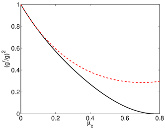
Figure 6: (Color online) $(g^{r}/g)^{2}$ as a function of $\mu_{c}$, full line according to Eq. (39) and dashed line according to Eq. (41) .

We see that there occurs a substantial suppression, such that already for $\mu_{c}=0.25$ the quantity $(g^{r}/g)^{2}$ is reduced to about a half of its value for $\mu_{c}=0$. Since $a^{2}>b$, the second term in Eq. (41) which dominates for larger $\mu_{c}$, leads to an upturn of the result. The result in Eq. (39) overestimate the suppression effect for large values of $\mu_{c}$.Huang et al. (2003) For the interacting system, the coefficients $a$ and $b$ tend to be smaller than the values in the non-interacting limit.

The vertex corrections $\Gamma^{(\rm ep)}_{U}$ also enter the electronic self-energy as one class of diagrams contributing to 3(c). This can be written as

$$\Sigma(i\omega_{n})=-\frac{1}{\beta}\sum_{m}\Gamma^{(\rm ep)}_{U}(i\omega_{n},i\omega_{m}+i\omega_{n})G(i\omega_{m}+i\omega_{n})D(i\omega_{m})\Gamma^{(\rm ep)}_{U}(i\omega_{m}+i\omega_{n},i\omega_{n}).$$ (42)

This is shown diagrammatically in Fig. 4 (b). As discussed above, there are also other types of mixed diagrams 3(d), which cannot be written in the form of Eq. (42).

III.3 Higher order corrections from purely $U$

We now deal with the higher order corrections purely from $U$, i.e., of type 4(a). We will restrict our attention only to the terms second order in $U$. The corresponding contribution (crossed diagram) to the pairing vertex reads

$$\Gamma^{(\rm pp)}(i\omega_{n_{1}},i\omega_{n_{2}};i\omega_{n}=0)=U^{2}\Pi(i\omega_{n_{1}}+i\omega_{n_{2}}).$$ (43)

The diagram is depicted in Fig. 7 (a).

Figure 7: (a) Higher order diagram vertex contribution from the Coulomb repulsion. (b) Second order in $U$ diagram for electronic self-energy.

A naive way of taking this into consideration would be to assume that $\Pi(i\omega_{n_{1}}+i\omega_{n_{2}})$ varies little for the scales under considerations, such that for all frequencies we can assume $-\rho_{0}U^{2}\Pi(0)=a\mu_{c}^{2}$. Then this term can be treated in the same way as the first order term in $U$, where we can simply write $\mu_{c}\to\bar{\mu}_{c}=\mu_{c}+a\mu_{c}^{2}$. This quantity is then subject to the full retardation effects and becomes $\bar{\mu}_{c}^{*}$,

$$\bar{\mu}_{c}^{*}=\frac{\bar{\mu}_{c}}{1+\bar{\mu}_{c}\log(\frac{D}{\omega_{\rm ph}})},$$ (44)

However, as analyzed in detail in Sec. V retardation effects are less efficient for the second order term when the decay of $\Pi(i\omega)$ is taken into account properly.

For the self-energy contributions of type 3(b), we will only consider the standard second order diagram depicted in Fig. 7 (b),

$$\Sigma(i\omega_{n})=-\frac{U^{2}}{\beta^{2}}\sum_{n_{1},n_{2}}G(i\omega_{n}-i\omega_{n_{1}})G(i\omega_{n_{1}}+i\omega_{n_{2}})G(i\omega_{n_{2}}).$$ (45)

IV Diagrammatic calculation for the superconducting state

In this section we consider calculations in the superconducting state. We first present the application of the standard theory to the HH model and then discuss higher order corrections. These calculations allow us, for instance, to study the gap at $T=0$. The relevant quantities are matrices in Nambu space. We have to calculate the diagonal and off-diagonal components of the self-energy. First we present the diagrams usually used in the standard ME approach.

IV.1 Standard diagrammatics, ME theory

To lowest order the diagonal self-energy is given by

$$\Sigma_{11}(i\omega_{n})=-\frac{g^{2}}{\beta}\sum_{m}G_{11}(i\omega_{m}+i\omega_{n})D(i\omega_{m}),$$ (46)

and the off-diagonal self-energy reads,

$$\Sigma_{21}(i\omega_{n})=\frac{g^{2}}{\beta}\sum_{m}G_{21}(i\omega_{m}+i\omega_{n})D(i\omega_{m}).$$ (47)

This is depicted in Fig. 8 (a) with the off-diagonal self-energy marked as $F$.

Figure 8: Diagrams for the off-diagonal self-energy (a) from electron-phonon interaction and (b) for the Coulomb repulsion with the notation $F=G_{21}$.

In the limit of low temperature, $T\to 0$, we use

$$\frac{1}{\beta}\sum_{n}f(i\omega_{n})\to\frac{1}{2\pi}\!\int\limits_{-\infty}^{\infty}\!\!{\rm d}\omega\;f(i\omega).$$ (48)

For the off-diagonal self-energy [see Fig. 8 (b)] we have the Coulomb contribution ($\eta\to 0$)

$$\Sigma_{21}(i\omega_{n})=\frac{U}{\beta}\sum_{m}G_{21}(i\omega_{m})\mathrm{e}^{i\omega_{m}\eta}.$$ (49)

Since $G_{21}(i\omega_{m})$ decays sufficiently rapidly the factor $\mathrm{e}^{i\omega_{m}\eta}$ is usually not needed.

These are the equations, which are taken into account in the standard theory. Often, the Coulomb term is then projected onto the phonon scale (Coulomb pseudopotential), where only the reduced value $\mu_{c}^{*}$ enters. Making a few simplifying assumption (see Sec. V.2) we can derive for the spectral gap at $T=0$, $\Delta_{\rm sp}\simeq\Sigma_{21}(0)/Z$,

$$\Delta_{\rm sp}=2\omega^{r}_{0}\mathrm{e}^{-\frac{Z}{\lambda-\mu_{c}^{*}(1+\frac{\lambda}{2})}}.$$ (50)

This result is very similar to the one for $T_{c}$. Equations (46), (47), and(49) correspond to the standard approach for the theory of conventional superconductivity.Carbotte (1990); Marsiglio and Carbotte (2008)

IV.2 Higher order corrections

In a similar way as for the analysis of the pairing vertex in Sec. III, we can classify terms for the self-energy into different contributions. We will follow the same logic as in the calculation for $T_{c}$ and focus on the same type of diagrams as before. Here we consider a subclass of type 3(c), which includes Coulomb vertex corrections of the electron-phonon vertex of the type $\Gamma^{(\rm ep)}_{U}$. It reads,

$$\Sigma_{11}(i\omega_{n})=-\frac{1}{\beta}\sum_{m}\Gamma^{(\rm ep)}_{U}(i\omega_{n},i\omega_{m}+i\omega_{n})G_{11}(i\omega_{m}+i\omega_{n})D(i\omega_{m})\Gamma^{(\rm ep)}_{U}(i\omega_{m}+i\omega_{n},i\omega_{n}).$$ (51)

Assuming a slow variation of $\Gamma_{U}$ on the phonon, scale a good approximation is of the form,

$$\Sigma_{11}(i\omega_{n})\simeq-\frac{[g^{r}]^{2}}{\beta}\sum_{m_{1}}D(i\omega_{m_{1}})G_{11}(i\omega_{n}+i\omega_{m_{1}}).$$ (52)

Similarly we have for the off-diagonal self-energy,

$$\Sigma_{21}(i\omega_{n})=\frac{1}{\beta}\sum_{m}\Gamma^{(\rm ep)}_{U}(i\omega_{n},i\omega_{m}+i\omega_{n})G_{21}(i\omega_{m}+i\omega_{n})D(i\omega_{m})\Gamma^{(\rm ep)}_{U}(i\omega_{m}+i\omega_{n},i\omega_{n}).$$ (53)

For $\Gamma^{(\rm ep)}_{U}(i\omega_{n},i\omega_{m})$ we consider the same diagrams as in Sec. III B. We assume that $D(i\omega_{m})$ is the full phonon propagator and hence it contains corrections due to $U$ as well.

IV.3 Higher order corrections from purely $U$

Of the contributions of the type 3(b) we discuss all terms to second order in $U$. In the Nambu perturbation theory ones has (cf. Ref. Martin-Rodero and Flores, 1992),

$$\Sigma_{11,U}^{(2,1)}(i\omega_{n})=-\Big{(}\frac{U}{\beta}\Big{)}^{2}\sum_{m_{1},m_{2}}G_{11}(i\omega_{n}+i\omega_{m_{1}})G_{22}(i\omega_{m_{2}})G_{22}(i\omega_{m_{1}}+i\omega_{m_{2}}).$$ (54)

and

$$\Sigma_{11,U}^{(2,2)}(i\omega_{n})=\Big{(}\frac{U}{\beta}\Big{)}^{2}\sum_{m_{1},m_{2}}G_{21}(i\omega_{n}+i\omega_{m_{1}})G_{12}(i\omega_{m_{2}})G_{22}(i\omega_{m_{1}}+i\omega_{m_{2}}).$$ (55)

For the off-diagonal part we have

$$\Sigma_{21,U}^{(2,1)}(i\omega_{n})=-\Big{(}\frac{U}{\beta}\Big{)}^{2}\sum_{m_{1},m_{2}}G_{21}(i\omega_{n}+i\omega_{m_{1}})G_{12}(i\omega_{m_{2}})G_{12}(i\omega_{m_{1}}+i\omega_{m_{2}}),$$ (56)

$$\Sigma_{21,U}^{(2,2)}(i\omega_{n})=\Big{(}\frac{U}{\beta}\Big{)}^{2}\sum_{m_{1},m_{2}}G_{11}(i\omega_{n}+i\omega_{m_{1}})G_{22}(i\omega_{m_{2}})G_{12}(i\omega_{m_{1}}+i\omega_{m_{2}}).$$ (57)

The first diagram $\Sigma_{11,U}^{(2,1)}(i\omega_{n})$ is the well known $U^{2}$-diagram which gives the first dynamic correction, also in the normal phase as in Eq. (45). In comparison $\Sigma_{11,U}^{(2,2)}(i\omega_{n})$ gives a smaller contribution as it is proportional to two off-diagonal Green’s function. $\Sigma_{21,U}^{(2,1)}(i\omega_{n})$ is also comparably small, but $\Sigma_{21,U}^{(2,2)}(i\omega_{n})$ gives a sizeable reduction of the superconducting state. We can see this by writing it as

$$\Sigma_{21,U}^{(2,2)}(i\omega_{n})=-U^{2}\frac{1}{\beta}\sum_{m_{1}}\Pi(i\omega_{n}+i\omega_{m_{1}})G_{21}(i\omega_{m_{1}}).$$ (58)

where $\Pi(i\omega_{n})$ is given in Eq. (32) with $G(i\omega_{m})=G_{11}(i\omega_{m})$.

For small $i\omega_{n}$ a crude approximation is to write

$$\Sigma_{21,U}^{(2,2)}(0)\simeq-U^{2}c_{1}\Pi(0)\frac{1}{\beta}\sum_{m_{1}}G_{21}(i\omega_{m_{1}}),$$ (59)

where it is assumed that $G_{21}(i\omega_{m_{1}})$ is only finite in small interval such that we can take $\Pi(i\omega_{n})$ constant. Hence we find a direct correction to the term $\Sigma_{21,U}^{(1)}$. With the result for $\Pi(0)$, one has then approximately

$$\Sigma_{21,U}^{(1)}+\Sigma_{21,U}^{(2,2)}(0)\simeq U(1+a\mu_{c})\frac{1}{\beta}\sum_{m_{1}}G_{21}(i\omega_{m_{1}}),$$ (60)

This is the same effect that was discussed for $T_{c}$ and the crossed diagram [see Fig. 7 (a)] where naively the effective $\mu_{c}$ becomes $\bar{\mu}_{c}=\mu_{c}(1+a\mu_{c})$. In a more accurate treatment, we have to take the frequency dependence into account, and we will see that this leads to modifications.

V Analytic and numerical results for $\mu_{c}^{*}$

In the last two sections we have analyzed the diagrammatic expansion for the model in Eq. (II) and discussed certain types of diagrams. In this section we want to specifically study the pseudopotential effect without including all other corrections. We are interested whether the first and second order calculations give qualitatively different results for $\mu_{c}^{*}$. We present a combination of analytical and numerical arguments. In the literature, there exist a number of ways to calculate $\mu_{c}^{*}$ for a given microscopic model. One early approach by Bogoliubov et al. is based on an integral equation for the Coulomb part in the pairing equation.Bogoliubov et al. (1962); Schrieffer (1964) Morel and Anderson Morel and Anderson (1962) gave an approximate solution for the Migdal-Eliashberg equations including a screened Coulomb repulsion in the $T=0$ formalism. The pseudopotential $\mu_{c}^{*}$ also appears naturally when superconducting pairing instabilities are studied in a renormalization group framework.Shankar (1994); Tam et al. (2007) In the following we first calculate $\mu_{c}^{*}$ directly by projecting the pairing matrix to low energy. Analytic and numerical results are compared. Then in a second approach we calculate $\Delta_{\rm sp}$ from an approximate solution of the self-consistency equation and thus extract $\mu_{c}^{*}$. Finally we also compute numerical results for $T_{c}$ obtained from the instability condition and analyze these results in terms of $\mu_{c}^{*}$.

V.1 Projection scheme

The starting point for the projection approach is the pairing matrix in the form

$$A_{nm}=\delta_{nm}-M_{nm},$$ (61)

where $M_{nm}$ is given in Eq. (13). This matrix becomes singular at $T_{c}$. We introduce the “low-energy part”

$$A^{\rm low}_{nm}=A_{nm}-\sum_{|\omega_{n}^{\prime}|,|\omega_{m}^{\prime}|>\omega_{\rm ph}}A_{nn^{\prime}}[\bar{A}^{-1}]_{n^{\prime}m^{\prime}}A_{m^{\prime}m},$$ (62)

$n,m$ such that $|\omega_{n}|,|\omega_{m}|<\omega_{\rm ph}$, and $\bar{A}$ is the matrix that is left after the blocks given by $|\omega_{n}|<\omega_{\rm ph}$ or $|\omega_{m}|<\omega_{\rm ph}$ were removed. If $\bar{A}^{-1}$ is not singular, Eq. (61) and Eq. (62) become singular for the same parameters. This way we can reduce the matrix size so that it only includes frequencies for which the electron-phonon interaction is important. The “folding in” of larger frequencies then describes how retardation effects reduce the effects of the Coulomb repulsion on low frequency properties.

We first consider the lowest order term of $\Gamma^{(\rm pp)}$ in $U$ namely $\Gamma^{(\rm pp)}=-U$. We want to focus on the dependence on the half-band width $D$ and assume that the density of states scales as

$$\rho(\varepsilon)={1\over 2D}\bar{\rho}\Big{(}{\varepsilon\over 2D}\Big{)},$$ (63)

where $\bar{\rho}$ is independent of $D$. For simplicity we assume in the following that $\bar{\rho}(x)=1$ is a constant for $|x|\leq 1/2$ and zero otherwise, such that $\rho_{0}=1/(2D)$. It is then a rather good approximation to write

$$\tilde{\chi}^{0}(i\omega_{n})=\begin{cases}\rho_{0}\pi/|\omega_{n}|,&\text{if $|\omega_{n}|<D$};\\ 0,&\text{otherwise.}\end{cases}$$ (64)

The matrix $A$ then takes the form

$$A_{nm}=\delta_{nm}+\frac{\pi}{\beta\sqrt{|\omega_{n}\omega_{m}|}}\mu_{c},$$ (65)

which is separable and can be inverted exactly. We obtain

$$[\bar{A}^{-1}]_{nm}=\delta_{nm}-\frac{\pi\mu_{c}}{\beta\sqrt{|\omega_{n}\omega_{m}|}[1+\pi\mu_{c}/\beta\sum_{k}^{{}^{\prime}}1/|\omega_{k}|]},$$ (66)

where $\sum_{k}^{{}^{\prime}}$ involves a summation over $|\omega_{k}|>\omega_{\rm ph}$. Replacing the summations in Eqs. (62, 66) by integrals, we find

$$A_{nm}^{\rm low}=\delta_{nm}+\frac{\pi}{\beta\sqrt{|\omega_{n}\omega_{m}|}}\mu_{c}$$

$$-\frac{\pi}{\beta\sqrt{|\omega_{n}\omega_{m}|}}\frac{\mu_{c}^{2}{\rm log}(D/\omega_{\rm ph})}{1+\mu_{c}{\rm log}(D/\omega_{\rm ph})}$$ (67)

$$=\delta_{nm}+\frac{\pi}{\beta\sqrt{|\omega_{n}\omega_{m}|}}\frac{\mu_{c}}{1+\mu_{c}{\rm log}(D/\omega_{\rm ph})}.$$

Comparison of Eq. (65) and (V.1) leads to the Coulomb pseudopotential, $\mu_{c}\to\mu_{c}^{*}$, as given in in Eq. (1), and it is the result of Morel and Anderson.Morel and Anderson (1962)

We next consider the second order term of $\Gamma^{(\rm pp)}$ in $U$ [Eq. (43)]. Because of the form of $\Pi(i\omega_{n}+i\omega_{m})$ it is then not possible to invert $\bar{A}$ in Eq. (62) analytically. For the density of states [Eq. (63)] we can rewrite $\Pi(i\omega_{n}+i\omega_{m})$ as

$$\Pi(i\omega_{n}+i\omega_{m})=-{1\over 2D}f\Big{(}\frac{\omega_{n}+\omega_{m}}{2D}\Big{)},$$ (68)

where $f$ is independent of $D$. As in Eq. (33) it is quite accurate to approximate $f$ as

$$f(x)=\frac{a}{1+b|x|+cx^{2}},$$ (69)

where $a=1.38$, $b=2$ and $c=5$ are suitable values for the constant DOS.

We now want to calculate $A^{\rm low}$ in Eq. (62) to third order in $U$. We use the result for $\bar{A}^{-1}$ in Eq. (66), which neglects the second order term and is therefore only correct to order $U$. However, since the off-diagonal terms of $A$ in Eq. (62) are of the order $U$, the final result is of the order $U^{3}$. We obtain

$$\sum_{nm}A_{1n}[\bar{A}^{-1}]_{nm}A_{m1}$$

$$=\tilde{\chi}^{0}(i\omega_{1})\Big{(}{U\over\beta}\Big{)}^{2}\sum_{|\omega_{n}|\geq\omega_{\rm ph}}\tilde{\chi}^{0}(i\omega_{n})\Big{[}1+\mu_{c}f\Big{(}{\omega_{n}\over 2D}\Big{)}\Big{]}^{2}$$

$$-\Big{(}{U\over\beta}\Big{)}^{3}{\tilde{\chi}^{0}(i\omega_{1})\over 1+\mu_{c}{\rm log}(D/\omega_{\rm ph})}$$ (70)

$$\times\Big{\{}\sum_{|\omega_{n}|\geq\omega_{\rm ph}}\tilde{\chi}^{0}(i\omega_{n})\Big{[}1+\mu_{c}f\Big{(}{\omega_{n}\over 2D}\Big{)}\Big{]}\Big{\}}^{2},$$

where we focus on the diagonal result for the lowest frequency $\omega_{1}$. Using the definition of $\tilde{\chi}^{0}(i\omega_{n})$ in Eq. (5), not the approximation in Eq. (64), and applying the limit $\omega_{\rm ph}\ll D$, we calculate the sums

$$\sum_{|\omega_{n}|\geq\omega_{\rm ph}}\tilde{\chi}^{0}(i\omega_{n})f\Big{(}{\omega_{n}\over 2D}\Big{)}^{k}={a^{k}\beta\over 2D}{\rm log}\Big{(}{DA_{k}\over\omega_{\rm ph}}\Big{)},$$ (71)

where $A_{0}\approx 1.00$, $A_{1}\approx 0.32$ and $A_{2}\approx 0.20$. For $k=1$ and 2 the denominator of $f$ reduces the integral for large $|\omega_{n}|$, which effectively reduces the band width by a factor $A_{k}$. This reduction is naturally larger for $k=2$ than for $k=1$.

We now make an ansatz for $\mu_{c}^{*}$

$$\mu_{c}^{*}=\frac{\mu_{c}+a\mu_{c}^{2}}{1+\mu_{c}\log\Big{(}\frac{D}{\omega_{\rm ph}}\Big{)}+a\mu_{c}^{2}\log\Big{(}\frac{D}{\omega_{\rm ph}}A_{22}\Big{)}},$$ (72)

along the lines of the Morel-Anderson form, but including a second order term and a corresponding logarithm. Based on Eq. (71) we expect the effective band width to be smaller for the second order term and we therefore allow for a different multiplying factor $A_{22}$ in the logarithm. Since the result in Eq. (V.1) is correct to order $U^{3}$ the factor $A_{22}$ in Eq. (72) can be identified, $A_{22}=A_{1}^{2}/A_{0}\approx 0.10$. The ansatz in Eq. (72) is then also correct to order $U^{3}$.

Fig. 9 shows the results obtained by performing the calculations in Eq. (62) numerically using the first or second order result in $U$ for $\Gamma^{(\rm pp)}$, and without introducing the approximation in Eq. (64). The figure also shows the analytical result in Eq. (72). The second order result is clearly larger than the first order result. For $\mu_{c}\lesssim 0.5$, Eq. (72) describes the full second order calculation rather well, while for larger $\mu_{c}$ there are corrections to the analytic result which make $\mu_{c}^{*}$ still larger compared to Eq. (72).

It is interesting to discuss the origin of the factor $A_{22}$ in Eq. (72). In the present language the term ${\rm log}(D/\omega_{\rm ph})$ in the first order calculation arises from “folding in” large frequency contributions from $U$ in Eq. (62), which extend to approximately $\omega\sim D$. The second order term in $U$ is “folded in” in a similar way. However, as shown by Eq. (69), the contribution from large frequencies is reduced, leading to the effective band width being reduced by some factor for the second order contribution. This reduction factor is surprisingly large (1/10). The origin can be seen in Eq. (V.1), where the relevant terms are a product of the first and second order contributions in the first term, containing a factor two, and the first order contribution in the second term. The prefactor two of the logarithm in the first contribution leads to the factor $A_{1}^{2}$, and thereby a very small factor.

This shows that the second order terms contribute to retardation effects, like the first order contribution. However, the reduction is substantially less efficient, as described by the small factor $A_{22}$. The band width therefore has to be very large to make this contribution to retardation efficient.

Figure 9: The pseudopotential $\mu^{*}_{c}$ as a function of $\mu_{c}$ for $D/\omega_{\rm ph}=100$ and $\beta\omega_{\rm ph}=240$. The figure shows the calculated results using both the first order and first plus second order result for $\Gamma^{(\rm pp)}$ as well as the approximation in Eq. (72).

It is interesting to consider the second order contribution alone. We can then calculate results accurate up to order $U^{4}$. The matrix $\bar{A}^{-1}$ can be approximated by a unit matrix. Making an ansatz for $\mu_{c}^{*}$ and identifying with the fourth order result, we obtain

$$\mu_{c}^{*}=\frac{a\mu_{c}^{2}}{1+a\mu_{c}^{2}{\rm log}\Big{(}\frac{DA_{2}}{\omega_{\rm ph}}\Big{)}},$$ (73)

where $A_{2}=0.20$ was given above. The result of a full calculation is compared with the analytical approximation [Eq. (73)] in Fig. 10. Also in this case the analytical result agrees rather well with the full calculation for $\mu_{c}\lesssim 0.5$.

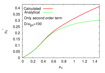
Figure 10: (Color online) $\mu^{*}_{c}$ as a function of $\mu_{c}$ for $D/\omega_{\rm ph}=100$ and $\beta\omega_{\rm ph}=240$. The figure shows the calculated value using just the second order result for $\Gamma^{(\rm pp)}$ as well as the analytical approximation in Eq. (73).

Finally, we compare the first and second order result as a function of $\log(D/\omega_{\rm ph})$ in Fig. 11. Different values for $\mu_{c}$ were used in the first and second order calculations, and chosen such that both calculations gave the same $\mu_{c}^{*}$ for $D/\omega_{\rm ph}=10$. It is quite interesting that $\mu_{c}^{*}$ then decreases in a very similar way in the two cases.

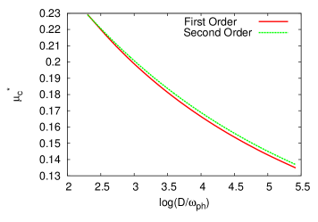
Figure 11: (Color online) $\mu_{c}^{*}$ as a function of $\log(D/\omega_{\rm ph})$ for $\beta\omega_{\rm ph}=240$ according to a first ($\mu_{c1}=0.5$) and second ($\mu_{c2}=0.2756$) order calculation. $\mu_{c1}$ and $\mu_{c2}$ were chosen so that the same $\mu_{c}^{*}$ was obtained in the two calculations for $D/\omega_{\rm ph}=10$.

We are now in the position to discuss the results for $\mu_{c}^{*}$. We have performed calculations using the first or second order expression for $\Gamma^{(\rm pp)}$. We then either calculated Eq. (62) numerically, without any further approximations. Alternatively, we performed analytical calculations involving the neglect of additional higher order terms in $U$.

When the first order result for $\Gamma^{(\rm pp)}$ is used, the analytical calculations can be performed without further approximations. This leads to the Morel-Anderson result, which has two important features. When $D/\omega_{\rm ph}\to\infty$, $\mu_{c}^{*}\to 0$, and when $U\to\infty$, $\mu_{c}^{*}\to 1/{\rm log}(D/\omega_{\rm ph})$ stays finite and saturates. Is this still true when the second order contribution to $\Gamma^{(\rm pp)}$ is included?

The analytical results in Eqs. (72,73) have these properties. However, these results were not derived but are ansätze inspired by the Morel-Anderson result and adjusted so that they agree with the analytical calculations to low order in $U$. Actually, Figs. 9,10 show that although retardation effects strongly reduce $\mu_{c}^{*}$, there is no sign that the values saturate as $U$ becomes very large. In this sense there is an important difference from the Morel-Anderson result. For these large values of $U$, higher order effects in $\Gamma^{(\rm pp)}$ become important, and it is not clear how these influence the conclusions.

The second issue is how $\mu_{c}^{*}$ is influenced when $D/\omega_{\rm ph}$ becomes very large. As is clear from Eqs. (72,73), retardation effects also reduce the second order contribution to $\mu_{c}^{*}$. This is also seen in Fig. 11. However, the effective band width is smaller due to the frequency dependence of the second order contribution and retardation effects are less efficient. Nevertheless, the second order contribution goes to zero as $D/\omega_{\rm ph}\to\infty$. In this context Fig. 11 may seem surprising. One might have expected the second order contribution to drop more slowly with $D/\omega_{\rm ph}$. To understand this one can study Eqs. (72,73) and find the $\mu_{c1}$ and $\mu_{c2}$ which lead to the same $\mu_{c}^{*}$ in the first and second order calculation. Because of the less efficient retardation effects for the second order term, $\mu_{c2}$ has to be chosen smaller than would otherwise have been the case. The criteria for the choice of $\mu_{c2}$ is, however, independent of $D$. Thus the two curves in Fig. 11 should be identical according to Eqs. (72,73). The small deviation is due to the inaccuracies of these analytical results for finite $U$. Fig. 11, nevertheless, nicely illustrates how both the first and second order contributions are systematically reduced as $D/\omega_{\rm ph}$ is increased.

V.2 Calculations for the gap at $T=0$

In this section we conduct a complimentary analysis to extract results for $\mu_{c}^{*}$. We calculate the spectral gap of the superconductor $\Delta_{\rm sp}$ at $T=0$, and show how $\mu_{c}^{*}$ enters naturally in the analytical description. We present this analysis to order $U^{2}$. The approach here is similar to the original work by Morel and Anderson,Morel and Anderson (1962) which included only the first order term in $U$ and was carried out in the $T=0$ formalism. Here, we work on the imaginary axis in the limit $T\to 0$. Starting point is the self-consistency equation for the off-diagonal self-energy,

$$\Sigma_{21}(i\omega_{n})=\frac{1}{\beta}\sum_{m}G_{21}(i\omega_{m})K(i\omega_{n},i\omega_{m}),$$ (74)

where the kernel $K(i\omega_{n},i\omega_{m})$ includes the following terms,

$$K(i\omega_{n},i\omega_{m})=g^{2}D(i\omega_{n}-i\omega_{m})+U-U^{2}\Pi(i\omega_{n}+i\omega_{m}).$$ (75)

The second and the third term are as given in Eq. (49) and Eq. (58). The expression for $G_{21}(i\omega_{m})$ was given in Eq. (15) and a semi-elliptic DOS is used in the following. We do not consider vertex corrections of the electron-phonon vertex here, and we simply use the form,

$$g^{2}D(i\omega_{n})=-\frac{\lambda}{\rho_{0}}\frac{1}{1+\big{(}\frac{\omega_{n}}{\omega_{\rm ph}}\big{)}^{2}}.$$ (76)

The effect of the diagonal self-energy is taken into account in the analytical calculations for completeness with a $Z$-factor for small frequencies, $|\omega_{n}|<\omega_{\rm ph}$. In the numerical calculations in this section it is neglected.

The self-consistency equation (74) can be solved numerically by iteration to find a solution for $\Sigma_{21}(i\omega_{n})$. For an analytical solution, we need to make some approximations. At half filling we use for the Green’s function for $|\omega_{n}|<\omega_{\rm ph}$,

$$G_{21}(i\omega_{n})\simeq-\frac{1}{t}\frac{\Sigma_{21}(i\omega_{n})}{\sqrt{Z^{2}\omega_{n}^{2}+\Sigma_{21}(i\omega_{n})^{2}}}$$ (77)

for $\omega_{\rm ph}<|\omega_{n}|<D$,

$$G_{21}(i\omega_{n})\simeq-\frac{1}{t}\frac{\Sigma_{21}(i\omega_{n})}{|\omega_{n}|}$$ (78)

and for $|\omega_{n}|>D$

$$G_{21}(i\omega_{n})\simeq-\frac{\Sigma_{21}(i\omega_{n})}{\omega_{n}^{2}}\simeq 0.$$ (79)

As discussed, $\Pi(i\omega)$ is well approximated by the form given in Eq. (33). As noted by Morel and AndersonMorel and Anderson (1962) the $\omega$-dependence of the off-diagonal self-energy is very similar to the one of the pairing kernel $K(i\omega_{n},i\omega_{m})$. Hence, a suitable ansatz for the off-diagonal self-energy is,

$$\Sigma_{21}(i\omega)=\Delta_{3}+\frac{\Delta_{2}}{1+b_{1}|\omega|+b_{2}\omega^{2}}+\frac{\Delta_{1}-\Delta_{2}-\Delta_{3}}{1+\big{(}\frac{\omega}{\omega_{\rm ph}}\big{)}^{2}}.$$ (80)

It contains the parameters $\Delta_{i}$. We assume that $b_{1}$ and $b_{2}$ take the same values as what is found for $\Pi(i\omega)$ in Eq. (33). By comparing the $\omega$-dependence with the full numerical solution we find reasonable accuracy for this assumption. In general we have to solve then for the parameters three $\Delta_{1}$, $\Delta_{2}$, and $\Delta_{3}$ by evaluating the self-consistency equation at suitable values of $i\omega$. Unfortunately, the general case is algebraically very involved. It will be discussed to some detail in the appendix. Here we only treat the first and purely second order cases to see the major effects.

For the first order case, we set $\Delta_{2}=0$ and omit the $U^{2}$-term in Eq. (75). We use the self-consistency equations $\Sigma_{21}(0)=\Delta_{1}$, and $\Sigma_{21}(iD)\simeq\Delta_{3}$. When evaluating the $\Sigma_{21}(0)$ and $\Sigma_{21}(iD)$ according to Eq. (74), we approximate the integrals in order to find an analytic solution (see appendix). We also assume $\Delta_{i}\ll\omega_{\rm ph}\ll D$ for simplification. Then for a self-consistent solution the parameters $\Delta_{1}$ and $\Delta_{3}$ have to satisfy the equations

$$\Delta_{1} = \frac{\lambda-\mu_{c}}{Z}\Delta_{1}\log\Big{(}\frac{2Z\omega_{\rm ph}}{\Delta_{1}}\Big{)}+a_{0}\lambda\Delta_{3}-\mu_{c}\Delta_{3}\log\Big{(}\frac{D}{\omega_{\rm ph}}\Big{)},$$

$$\Delta_{3} = -\mu_{c}\Big{[}\frac{\Delta_{1}}{Z}\log\Big{(}\frac{2Z\omega_{\rm ph}}{\Delta_{1}}\Big{)}+\Delta_{3}\log\Big{(}\frac{D}{\omega_{\rm ph}}\Big{)}\Big{]}.$$ (81)

The coefficient $a_{0}$ is given in the appendix. This yields the non-trivial solutions

$$\Delta_{1}=2Z\omega_{\rm ph}\mathrm{e}^{-\frac{Z}{\lambda-\mu_{c}^{*}(1+a_{0}\lambda)}},\;\;\Delta_{3}=-\frac{2Z\omega_{\rm ph}\mu_{c}^{*}}{\lambda-\mu_{c}^{*}}\mathrm{e}^{-\frac{Z}{\lambda-\mu_{c}^{*}(1+a_{0}\lambda)}},$$ (82)

where the standard result for $\mu_{c}^{*}$ is obtained,

$$\mu_{c}^{*}=\frac{\mu_{c}}{1+\mu_{c}\log(\frac{D}{\omega_{\rm ph}})}.$$ (83)

Note that the gap in the spectral function $\Delta_{\rm sp}$, found from the pole of the Green’s function, occurs at $|\omega|=\Delta_{1}/Z$ in this approximation.

Accounting for the approximations made in this derivation we can use this form with three fitting parameters as in Eq. (27),McMillan (1968)

$$\Delta_{\rm sp}=c_{1}\omega_{\rm ph}\mathrm{e}^{-\frac{Zc_{2}}{\lambda-\mu_{c}^{*}(1+c_{3}\lambda)}},$$ (84)

where $c_{1}>0$, $c_{2}>1$. We can determine the parameters $c_{1}$, $c_{2}$ by fitting to the numerical solution of Eq. (74) for $\mu_{c}=0$ in the regime $0<\lambda<0.5$. Note that in contrast to the analytical solution the result of the numerical solution depends in general on the bandwidth $W$. It only becomes independent in the large bandwidth limit.Marsiglio (1990)

For $\mu_{c}=0$, $D=8/\omega_{\rm ph}=80$, we find with $c_{1}=1.7$, $c_{2}=1.07$ good agreement of the formula (84) with the numerical results for $\lambda<0.5$ as can be seen in Fig. 12. Note that for the Holstein model and larger values of $\lambda$, the result in Eq. (84) underestimates $\Delta_{\rm sp}$ as already pointed out by Allen and Dynes.Allen and Dynes (1975)

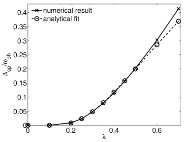
Figure 12: The spectral gap $\Delta_{\rm sp}$ as calculated from the numerical solution of Eq. (74) as a function of $\lambda$ for $D/\omega_{\rm ph}=80$ in comparison with the analytical form in Eq. (84) with the the parameters $c_{1}=1.7$, $c_{1}=1.07$.

For fixed $\lambda=0.5$, we also compare the $\mu_{c}$-dependence of the analytical result in Eq. (84) with the full numerical solution. In Fig. 13 a comparison can be found, where we used the same values for $c_{1}$ and $c_{2}$ as for $\mu_{c}=0$ and found that $c_{3}=0.8$ gives a reasonable fit.

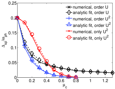
Figure 13: (Color online) The spectral gap $\Delta_{\rm sp}$ as calculated from the numerical solution of Eq. (74) with different kernels as a function of $\mu_{c}$ for $D/\omega_{\rm ph}=80$ in comparison with the analytical result in Eq. (84).

We analyze the situation including only the $U^{2}$-term now. We set $\Delta_{3}=0$ in this case and omit the constant $U$-term in Eq. (75). To determine the parameters $\Delta_{1}$ and $\Delta_{2}$, we use the following two conditions: $\Sigma_{21}(0)=\Delta_{1}=\sum_{i}N_{1i}\Delta_{i}$, and $\Sigma_{21}(iD)+\Sigma_{21}(-iD)\simeq 2\Delta_{2}/(1+b_{1}D+b_{2}D^{2})=\sum_{i}N_{2i}\Delta_{i}$. This yields the self-consistency equation,

$$1=N_{11}+\frac{N_{12}N_{21}}{\frac{2}{1+b_{1}D+b_{2}D^{2}}-N_{22}}.$$ (85)

Making similar approximation as in the first order calculation we find for the coefficients $N_{ij}$,

$$N_{11}=\frac{1}{Z}(\lambda-a\mu_{c}^{2})\log(T_{1}),$$ (86)

and

$$N_{21}=-\frac{2}{Z}\frac{a\mu_{c}^{2}}{1+b_{1}D+b_{2}D^{2}}\log(T_{1}).$$ (87)

with

$$T_{1}=\frac{Z\omega_{\rm ph}+\sqrt{(Z\omega_{\rm ph})^{2}+\Delta_{1}^{2}}}{\Delta_{1}}.$$ (88)

One also finds

$$N_{12}=a_{12}\lambda-a\mu_{c}^{2}\log\Big{(}\frac{D}{\omega_{\rm ph}}\bar{A}_{12}\Big{)},$$ (89)

and

$$N_{22}=-a\mu_{c}^{2}\frac{2}{1+b_{1}D+b_{2}D^{2}}\log\Big{(}\frac{D}{\omega_{\rm ph}}\bar{A}_{22}\Big{)}.$$ (90)

The expressions for $a_{12}$, $\bar{A}_{12}$ and for $\bar{A}_{22}$ can be found in the appendix. The coefficients $\bar{A}_{12}<1$ and $\bar{A}_{22}<1$ appear due to additional terms to $1/\omega$ in the integrand which accelerate the decay towards higher energy. Hence, they lead to a reduced effective bandwidth, $D\to\bar{A}_{22}D$ as discussed in the previous section. The solution of Eq. (85) yields

$$\Delta_{1}=2Z\omega_{\rm ph}\mathrm{e}^{-\frac{Z}{\lambda-\mu_{c}^{*}(1+a_{12}\lambda)-\mu_{c,1}^{*}}},$$ (91)

with

$$\mu_{c}^{*}=\frac{a\mu_{c}^{2}}{1+a\mu_{c}^{2}\log\Big{(}\frac{D}{\omega_{\rm ph}}\bar{A}_{22}\Big{)}},$$ (92)

and

$$\mu_{c,1}^{*}=\frac{\log(\frac{\bar{A}_{22}}{\bar{A}_{12}})a^{2}\mu_{c}^{4}}{1+a\mu_{c}^{2}\log\Big{(}\frac{D}{\omega_{\rm ph}}\bar{A}_{22}\Big{)}}.$$ (93)

The result for $\mu_{c}^{*}$ has the same form as what was derived in Eq. (73). In addition a higher order term $\mu_{c,1}^{*}$ appears. In the first order calculations all higher order contributions cancel in the numerator of the expression for $\mu_{c}^{*}$. However, in the second order calculation this is not the case anymore and an additional term remains. The coefficient $\log(\bar{A}_{22}/\bar{A}_{12})$ does not increase with the bandwidth $W$ and therefore the whole term becomes small in the large bandwidth limit due to the logarithm in the denominator. For the relevant values one has $\bar{A}_{22}/\bar{A}_{12}\approx 2$ such that the coefficient of the $\mu_{c}^{2}$ is relatively small and the term does not contribute much for small values of $\mu_{c}$. For larger values, however, it does play a role. Thus it can account for the discrepancy between the numerical and the analytical result from Eq. (73) observed in Fig. 10, where the numerical result does not seem to saturate.

We would like to check these analytical findings with the full numerical solution of the self-consistency equation. Formally, we had found very similar results to the ones of the last section derived from the projection scheme. For the comparison with the numerics we take these expressions and use the values for the parameters derived there, i.e. we use $\bar{A}_{22}\to A_{2}$ , where $A_{2}=0.197$ or $\log(A_{22})=-1.624$. We omit the term $\mu_{c,1}^{*}$, and for $c_{1}$, $c_{2}$ we take the same values as above, and we use $a_{12}=c_{3}$. The reason for this procedure is that due to a number of approximations involved in the analytic calculation the results for these coefficient do not tend to be very accurate. Moreover, we aim for a unified description with as little parameters as possible.

The result for the “only $U^{2}$”-calculation is added in Fig. 13 and compared with the full numerical solution. We find good agreement. For small values of $\mu_{c}$ the reduction of $\Delta_{\rm sp}$ is smaller than for the first order term, but then $\Delta_{\rm sp}$ drops more rapidly. Notice that the second order result for $\mu_{c}^{*}$ is analogous in the form to the first order calculation. The difference is the factor $\bar{A}_{22}<1$ in the logarithm in the denominator. Hence, the retardation effects are less effective in this case as discussed in the previous section. The results here are derived independently from the arguments of the last section, but are fully consistent with them. The higher order term $\mu_{c,1}^{*}$ is not very important for the values of $\mu_{c}$ appearing in Fig. 13.

In the general case including both the first and second order terms in Eq. (75), we have to solve for three parameters and hence have three self-consistency equations to be solved. In general this can be written as a matrix equation $\bm{\Delta}=\underline{M}\bm{\Delta}$. Algebraically this becomes rather lengthy and yields a number of different terms for $\mu_{c}^{*}$, as discussed in the appendix. To simplify the discussion, we use results in the form of Eq. (84) with $\mu_{c}^{*}$ as introduced in Eq. (72),

$$\mu_{c}^{*}=\frac{\mu_{c}+a\mu_{c}^{2}}{1+\mu_{c}\log(\frac{D}{\omega_{\rm ph}})+a\mu_{c}^{2}\log\Big{(}\frac{D}{\omega_{\rm ph}}A_{22}\Big{)}},$$ (94)

for comparison with the numerical results. In Fig. 13 we have included the numerical result of Eq. (74) with the full kernel in Eq. (75). We also included the analytical description based on Eq. (84) and (72) with the same value $\log(A_{22})=-2.28$ or $A_{22}=0.1022$ as in the previous section. We find a rather good agreement for the range of values of $\mu_{c}$.

We can accurately calculate the dependence of the spectral gap $\Delta_{\rm sp}$ on $\mu_{c}$ for given $\lambda$, $D$ and $\omega_{\rm ph}$ numerically. However, it is not possible to calculate $\mu_{c}^{*}$ directly from the self-consistency equation (74). If we assume that the form of Eq. (84), which neglects higher order terms of the form Eq. (93), gives a good description and we can solve for $\mu_{c}^{*}$,

$$\mu_{c}^{*}=\frac{\lambda}{1+c_{3}\lambda}+\frac{Zc_{2}}{\log\Big{(}\frac{\Delta_{\rm sp}}{c_{1}\omega_{\rm ph}}\Big{)}(1+c_{3}\lambda)}.$$ (95)

As higher order terms are neglected this is not the complete result for $\mu_{c}^{*}$ for the whole range of $\mu_{c}$. However, if $\mu_{c}^{*}$ is interpreted as the quantity in competition with $\lambda$ to cause superconductivity, then this form is useful and the inversion of Eq. (84) can give us an estimate for $\mu_{c}^{*}$.

The results for $\mu_{c}^{*}$ obtained from Eq. (95) together with the analytical estimates in Eqs. (1,73,72) can be found in Fig. 14.

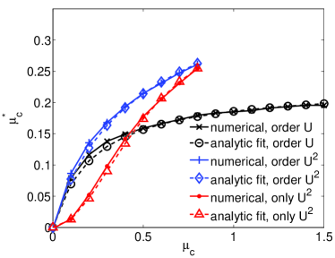
Figure 14: (Color online) $\mu_{c}^{*}$ as a function of $\mu_{c}$ for $D/\omega_{\rm ph}=80$ computed from Eq. (95). We show in comparison the result for the first order and the second order calculation. The fit parameters are $c_{1}$, $c_{2}$ and $c_{3}$ are the same as above.

The results look very similar to the ones in the previous section in Fig. 9. For small $\mu_{c}$, $\mu_{c}^{*}$ increases linearly with $\mu_{c}$ in Eqs. (1,72). This implies an initially relatively large drop of superconductivity once the Coulomb repulsion becomes finite (see Fig. 13). However, then the curves bend and the analytical results saturate. Only for very small values of $\mu_{c}$ the first and second order results are in agreement, otherwise the second order result is substantially larger. For the first order calculation the upper boundary is given by $\mu_{c,\rm max}^{*}=1/\log(\frac{D}{\omega_{\rm ph}})$ independent of $\mu_{c}$. It is reached both in the limit of large $\mu_{c}$ and large ratio $D/\omega_{\rm ph}$. For instance for $D/\omega_{\rm ph}=1000$, we have $\mu_{c,\rm max}^{*}\approx 0.145$, similar to what is usually used in the literature. Using $\mu_{c}=0.5$ for the screened Coulomb interaction gives with the same ratio for $D/\omega_{\rm ph}$ the value $\mu_{c}^{*}=0.112$ (see Tab. 2).

$D/\omega_{\rm ph}$	10	100	1000
$\mu_{c}^{*}$ in Eq. (1)	0.232	0.151	0.112
$\bar{\mu}_{c}^{*}$ in Eq. (44)	0.286	0.172	0.123
$\mu_{c}^{*}$ in Eq. (72)	0.386	0.204	0.139

Table 1: Exemplary values for $\mu_{c}^{*}$ for $\mu_{c}=0.5$.

$D/\omega_{\rm ph}$	10	100	1000
$\mu_{c}^{*}$ in Eq. (1)	0.303	0.172	0.127
$\bar{\mu}_{c}^{*}$ in Eq. (44)	0.366	0.199	0.136
$\mu_{c}^{*}$ in Eq. (72)	0.700	0.268	0.166

Table 2: Exemplary values for $\mu_{c}^{*}$ for $\mu_{c}=1$.

We can see that the higher order results for $\mu_{c}^{*}$ are generally substantially larger than in the first order calculation. In particular the results are larger than the simple minded estimate, $\bar{\mu}_{c}^{*}$ in Eq. (44), where retardation effects are the same for the first and second order term. For this expression the limits of large bandwidth and large $\mu_{c}$ lead to the same result $\bar{\mu}_{c,\rm max}^{*}=1/\log(\frac{D}{\omega_{\rm ph}})$, which is however reached already for smaller values, e.g. for $\mu_{c}=0.5$ we have $\bar{\mu}_{c}^{*}=0.1233$. In contrast, the result in Eq. (72) goes to $\mu_{c,\rm max}^{*}=1/\log(\frac{D}{\omega_{\rm ph}}A_{22})$ in the limit of large $\mu_{c}$ and to $\mu_{c,\rm max}^{*}=1/\log(\frac{D}{\omega_{\rm ph}})$ in the limit of a very large bandwidth. With the estimate for $A_{22}$ above we find for $D/\omega_{\rm ph}=1000$ that in the large $\mu_{c}$ limit $\mu_{c,\rm max}^{*}\approx 0.216$ is about 50 % larger than the first order estimate. For comparison we give some results in tables 2 and 2 for $\mu_{c}=0.5$, $\mu_{c}=1$, and the ratios $D/\omega_{\rm ph}=10,100,1000$. Notice, that the more accurate result for $\mu_{c}^{*}$ as obtained from the numerical calculation and shown in Fig. 9 can be still significantly larger than the estimate in Eq. (72). We conclude that the usual result in Eq. (1) substantially underestimates $\mu_{c}^{*}$ for intermediate and larger values of $\mu_{c}$. However, for very large values of $D/\omega_{\rm ph}$ retardation effects are operative in all cases and lead to a strongly reduced value of $\mu_{c}^{*}$.

V.3 Calculations for $T_{c}$

For completeness we also include a brief section on the critical temperature $T_{c}$. It is analyzed similar to the last section. The basis for the calculations is the pairing matrix in Eq. (13). For the pairing vertex we use the same terms as in the previous section in Eq. (75),

$$\Gamma^{(\rm pp)}(i\omega_{n_{1}},i\omega_{n_{2}};0)=-K(i\omega_{n_{1}},i\omega_{n_{2}}).$$ (96)

The effect of the $Z$-factor is neglected. Then with the bare Green’s function and a semi-elliptic DOS

$$\tilde{\chi}^{0}(i\omega_{n_{1}};0,0)=-\frac{G(i\omega_{n_{1}})}{i\omega_{n_{1}}}=\rho_{0}\frac{\pi}{2t}\left(\sqrt{1+\frac{4t^{2}}{\omega_{n}^{2}}}-1\right).$$ (97)

$\Pi(i\omega_{n})$ is calculated numerically from the free Green’s function. With this we compute the matrix $M_{n_{1},n_{2}}$ in Eq. (13) and search for the largest eigenvalue. We compare the results for $T_{c}$ for three different calculations: (1) including only the $U$-term, (2) including only the $U^{2}$-term and (3) including both.

Apart from the first order calculation it is not easy to find a good analytic approximation for the eigenvalue equation (12). In principle, one can do something similar to what has been done in the last section and make an appropriate ansatz for the eigenvector. To first order in $U$ this works reasonably well. We find a result of the standard form,

$$T_{c}=c_{1}\omega_{\rm ph}\mathrm{e}^{-\frac{Zc_{2}}{\lambda-\mu_{c}^{*}(1+c_{3}\lambda)}}.$$ (98)

where $\mu_{c}^{*}$ is given by Eq. (83). For the higher order analysis we did not pursue an analytical solution, and instead also assume $T_{c}$ as in Eq. (98) and for $\mu_{c}^{*}$ the form in Eq. (72).

First we fix the constants $c_{1}$ and $c_{2}$ by fitting to the result for $\mu_{c}=0$, see Fig. 15. We take the value $c_{1}=1/1.2\approx 0.833$ as in Ref. Allen and Dynes, 1975 and find a good fit for $c_{2}=1.04$. Similar as before the agreement is only good up to values of $\lambda<0.5$.

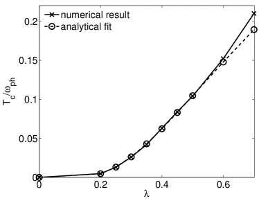
Figure 15: (Color online) $T_{c}$ as a function of $\lambda$ for $D/\omega_{\rm ph}=80$.

In Fig. 16 we give the numerical result for $T_{c}$ as a function of $\mu_{c}$ for the first order calculation, only the second order and first plus second order. We have kept $\lambda=0.5$ constant.

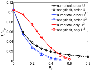
Figure 16: (Color online) $T_{c}$ as a function of $\mu_{c}$ for $D/\omega_{\rm ph}=80$.

$T_{c}$ decays in a very similar way as the spectral gap when $\mu_{c}$ is increased. We included results from the analytic fit form in Eq. (98) with the value $c_{3}=0.8$. For the first order calculation, we find good agreement with the numerical result for the case $\lambda=0.5$. For the second order results we use the same parameters as before and the fits are reasonable, i.e. they show that the functional form is close to the actual result.

Note, that in spite of the identical form for the pairing kernel, the results for $T_{c}$ here and the ones for the gap at $T=0$ in the previous section are obtained from two independent calculations. The results indicate that for the range of parameters studied the analytical expressions Eqs. (1,73,72) describe the effect of $\mu_{c}^{*}$ on $T_{c}$ quite accurately. In particular the results are very similar to what has been found in the projective approach before, and hence a consistent picture emerges. We conclude that higher order dynamic effects, and in particular the second order contributions, give an important correction to the usual results for the Coulomb pseudopotential. Not only does the higher order term give a direct increase of the coupling, as would be the case in expression in Eq. (44) it also leads to a reduced effective bandwidth in the logarithm in the denominator. This is an effect which to our knowledge has not been discussed in the literature so far. In the following section we analyze how these effects are manifest in the non-perturbative DMFT calculations.

VI DMFT and perturbative results

In this section we put the analysis of the previous sections together and compare with non-perturbative DMFT calculations, which include all possible renormalization effects. We first clarify that it is therefore very important to work with renormalized parameters for the interpretation of the results. Then we demonstrate up to which interaction strengths the perturbative results derived in the previous section are reliable.

We focus on calculations for the spectral gap $\Delta_{\rm sp}$ at $T=0$ and consider a half filled band. The spectral gap $\Delta_{\rm sp}$ is extracted directly from the gap edges of the diagonal spectral function. It is usually well approximated by the product $z\Sigma_{21}(0)$, but it can be a bit larger due to the frequency dependence of the off-diagonal self-energy. For an interpretation of the DMFT results we need to compare with the perturbation theory (PT) results. We include the following terms for the self-consistent PT calculation: For the diagonal and off-diagonal self-energy we use Eqs. (51) and (53). The vertex is approximated by the contributions from RPA screening in Eq. (34) up to second order in $U$ and the second order in $U$ corrections in Fig. 5. For a small phonon frequency, the $\omega=0$ value of the vertex function provides a good approximation. From the diagrams in $U$ we take Eqs. (49), and (54)-(57) into account. The phonon propagator is taken as an input from DMFT calculations and not calculated self-consistently, similar to what has been done in Ref. Bauer et al., 2011.

To get a feeling for the renormalization effects let us first consider calculations, where the bare parameters $\lambda_{0}=\rho_{0}2g^{2}/\omega_{0}$ and $\omega_{0}$ in the Hamiltonian (II) are kept fixed. For $\mu_{c}=0$ the system has a superconducting solution and we analyze how the gap $\Delta_{\rm sp}$ is affected, when $\mu_{c}$ becomes finite. For $\lambda_{0}=0.308$ and $\lambda_{0}=0.382$, the corresponding spectral gaps $\Delta_{\rm sp}$ are shown in Fig. 17. For comparison we have also included the results from the self-consistent PT as explained above in Fig. 17. These are seen to be in very good agreement with the DMFT result.

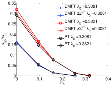
Figure 17: (Color online) Behavior of the spectral gap $\Delta_{\rm sp}$ and $z\Sigma^{\rm off}(0)$ for constant $\lambda_{0}=0.308$ and $\lambda_{0}=0.382$ ($\omega_{0}=0.1$ in both cases) as a function of $\mu_{c}$.

We find a rapid decrease of $\Delta_{\rm sp}$ when $\mu_{c}$ becomes finite, similar to the results in Fig. 13. However, notice that $\Delta_{\rm sp}$ goes to zero for even smaller values of $\mu_{c}\sim 0.3$. Naively one could conclude that $\mu_{c}^{*}$ is even larger than what was discussed in the last section even though we are still at very weak coupling in $U$. As we will see, however, this drastic reduction of $\Delta_{\rm sp}$ has a different origin. It can be understood by analyzing the relevant effective parameters and the PT results.

Since, as shown in Sec. V many aspects of the PT are well described by approximate analytical results, such as Eq. (72) for $\mu_{c}^{*}$ or Eq. (84) for $\Delta_{\rm sp}$, it makes sense to use those equations to analyze the results. In Sec. V the equations were used in terms of bare parameters, but to understand the DMFT results we need to use renormalized parameters. Those effective parameters extracted from the DMFT calculation are shown in Fig. 18 as function of $\mu_{c}$.

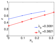
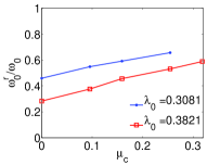
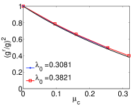
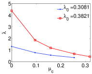
Figure 18: (Color online) The effective parameters (a) the quasiparticle renormalization $z$, (b) the renormalized phonon frequency $\omega_{0}^{r}/\omega_{0}$ (c) the renormalized coupling constant $(g^{r}/g)^{2}$ (the full line corresponds to the result with $a$ and $b$ obtained from the free Green’s functions) and (c) the effective $\lambda$ as a function of $\mu_{c}$.

The $z$-factor in Fig. 18 (a) increases moderately with $\mu_{c}$. According to Eq. (84) with $Z=z^{-1}$ this would actually help superconductivity, so it can not be responsible for the reduction in Fig. 17. The renormalized phonon frequency $\omega_{0}^{r}$ in Fig. 18 (b) also increases with $\mu_{c}$ showing that corrections to the phonon self-energy and electron-phonon vertex from finite $U$ are important. In the prefactor of Eq. (84) with $\omega_{\rm ph}=\omega_{0}^{r}$ this leads to an enhancement of $\Delta_{\rm sp}$, whereas $\mu_{c}^{*}$ increases with $\omega_{0}^{r}$ which leads to a reduction of $\Delta_{\rm sp}$. Both effects are not strong enough to be decisive. The strongest and most important effect of $\mu_{c}$ can be seen in Fig. 18 (c) and (d), where we plot the renormalized coupling $g^{r}$ from Eq. (39) and the effective $\lambda$ according to Eq. (29). The parameters $a$ and $b$ in Eq. (39) are calculated from the full Green’s functions. We find that the renormalized coupling $g^{r}$ decreases substantially with $\mu_{c}$. In addition the phonon self-energy is modified for finite $U$. Therefore, the effective $\lambda$ becomes much smaller. So the main reason for the rapid suppression of $\Delta_{\rm sp}$ is the strong effect of the corrections to the electron-phonon vertex and to the phonon self-energy, such that the effective $\lambda$ decreases.

Using values $\omega_{\rm ph}=\omega_{0}^{r}$ we can calculate results for the Coulomb pseudopotential $\mu_{c}^{*}$ according to Eq. (72). The ratio of electron over phonon scale is with $D/\omega_{0}^{r}\sim 35$ not as large as in the last section, and thus retardation effects not as effective. For the largest value $\mu_{c}\simeq 0.318$ we find $\mu_{c}^{*}\simeq 0.2$. At this $\mu_{c}$ we have $\lambda\simeq 0.45$ and the analytic expression in Eq. (84) yields $\Delta_{\rm sp}/\omega_{0}\simeq 0.0002$, where $Z=z^{-1}$, $\omega_{\rm ph}=\omega_{0}^{r}$, and for the fitting parameters $c_{i}$ take the same values as in Sec. V.2. This is in agreement with the DMFT finding that superconductivity goes to zero then. If we compare the results for the spectral gap according to Eq. (84) with the renormalized parameters in Fig. 18 with the results from the full calculation in Fig. 17 we find good agreement. Hence we conclude that the superconducting state at small $\mu_{c}$ can be well understood in terms of the effective parameters $\lambda$, $\omega_{0}^{r}$, $z$ and $\mu_{c}^{*}$ and the approximate equations for $\mu_{c}^{*}$ and $\Delta_{\rm sp}$.

The conclusion up to this stage is that the strongest effect of the Coulomb repulsion in the DMFT calculations is to renormalize the effective $\lambda$ via electron-phonon vertex and phonon propagator such that superconductivity drops to zero rapidly. Even at very weak coupling these effects play an important role in the Hubbard-Holstein model and must be taken into account. Since in this work our main interest is the effectiveness of retardation effects visible in the direct competition between $\lambda$ and $\mu_{c}^{*}$, we will offset the vertex-correction effect in the following. We do this by appropriately adjusting the bare parameters, i.e., increasing $\lambda_{0}$ and $\omega_{0}$. We proceed by keeping $\lambda=\lambda(\mu_{c})$ as defined in Eq. (29) constant. For $g^{r}$ we rely on the perturbative results. This was found to give a relatively good description up to $U\sim W/2$.Huang et al. (2003) First we do a calculation for certain bare values $\omega_{0}$ and $\lambda_{0}$ at $\mu_{c}=0$. From the phonon spectral function we can then extract the value $\omega_{0}^{r}$ and $\lambda$ from (29) where, $g^{r}=g$. Then we choose a finite value of $\mu_{c}$. We have to increase $\lambda_{0}$ and $\omega_{0}$, such that $\omega_{0}^{r}$ roughly equals the $U=0$ value and $\lambda$ remains approximately the same according to Eq. (29). For the renormalized coupling $g^{r}$ entering Eq. (29) we consider two conditions: (a) the second order expansion as in Eq. (41) and (b) the RPA series plus the second order terms as in Eq. (39). With the set of bare parameters $(\lambda_{0},\omega_{0},\mu_{c})$ found from this procedure we also do perturbative calculations for comparison. We distinguish PT-a, which includes up to second order diagrams for the electron-phonon vertex, and PT-b which includes the RPA series plus the second order terms for the electron-phonon vertex. The results of such a calculation, where $\lambda\simeq 1$ according to condition (a) and $\omega_{0}^{r}/D\simeq 0.025$ are shown in Fig. 19 as $\Delta_{\rm sp}$ vs $\mu_{c}$.

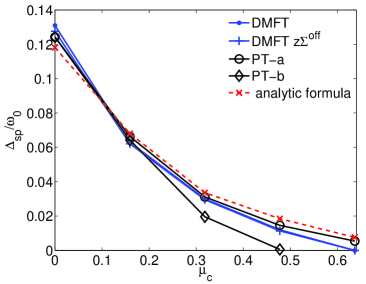
Figure 19: (Color online) Behavior of the DMFT result for the spectral gap $\Delta_{\rm sp}$ and $z\Sigma^{\rm off}(0)$ for constant $\lambda\simeq 1$ according to condition (a) for the vertex corrections (see text), $\omega_{0}^{r}\simeq 0.05$ as a function of $\mu_{c}$ in comparison with PT-a and PT-b (see text) and the analytic formula in Eq. (84).

The DMFT results show a steady decrease of $\Delta_{\rm sp}$ on increasing $\mu_{c}$. Since the effective $\lambda$ and $\omega_{\rm ph}$ are kept constant the diminution of $\Delta_{\rm sp}$ is now due to the competition with the Coulomb repulsion $\mu_{c}$. To understand the result quantitatively we compare it with the perturbative calculations PT-a, PT-b and the analytic results based on Eq. (84) using the effective parameters and $\mu_{c}^{*}$ according to Eq. (72) with the value of $A_{22}$ as in Sec. V. We find a relatively good agreement of the DMFT result with PT-a and the analytic formula up to $\mu_{c}\sim 0.5$. This demonstrates that (i) the effective parameter description is appropriate, (ii) the electron-phonon vertex correction according to condition (a) is suitable and (iii) that the derived higher order form for the Coulomb pseudopotential in Eq. (72) captures correctly the results of the PT and the of the full DMFT calculation. This validates the analysis of the Sec. V in a more complete calculation and it corroborates our findings for $\mu_{c}^{*}$ and retardation effects by comparison with non-perturbative DMFT up to intermediate values of $\mu_{c}\sim 0.5$. For larger values of $\mu_{c}$, higher order correction enhance the value of $\mu_{c}^{*}$ such that $\Delta_{\rm sp}$ is suppressed stronger. In addition the electron-phonon vertex is not well described by condition (a) anymore. The PT-b calculation agrees with DMFT quite well up to values $\mu_{c}\sim 0.3$, but then overestimates the reduction of the electron-phonon vertex and therefore leads to a too strong suppression of superconductivity.

To extend the present analysis to larger values of $\mu_{c}$, one needs to find reliable estimates for the full renormalized electron-phonon vertex $\Gamma^{(\rm ep)}_{U}$. A higher order perturbative analysis or non-perturbative calculation for this quantity could provide this. A consistent calculation up to certain order in $\mu_{c}$ should then also include higher order corrections to the self-energies, which will complicate the analytical calculation for $\mu_{c}^{*}$ further. This is beyond the scope of this work.

VII Conclusions

For the occurrence of conventional superconductivity it is important that on the one hand there is a sizeable electron-phonon coupling and on the other that the detrimental effects of the Coulomb repulsion are reduced sufficiently by screening and retardation effects. We have stressed in this article that while the effect of the former can be described in a controlled fashion by Migdal-Eliashberg theory, the standard approach to the latter is based on an uncontrolled approximation, since there is no Migdal theorem for the Coulomb interaction. For the Hubbard-Holstein model we have analyzed this issue in a controlled framework by a combination of perturbative calculations and non-perturbative DMFT calculations. We have shown that the conventional arguments based on the lowest order diagrams become modified when higher order corrections are taken into account. There is still a reduction of the Coulomb repulsion due to logarithmic terms in the denominator. This demonstrates that indeed a small value of $\mu_{c}^{*}$ can be obtained due to retardation effects even when higher order corrections are considered. Thus our results support the arguments by Morel and Anderson qualitatively. However, the effective energy scale separation is reduced. This is due to the dynamic behavior of the higher order diagrams which make retardation effects less operative. This result was shown explicitely in two independent calculations in a combination of analytical and numerical arguments. By studying the occurrence of superconductivity with DMFT, where all higher order corrections are present, we were able corroborate our findings up to intermediate coupling strength. The perturbative approach allowed us to distinguish different renormalization effects. Our analysis is limited to intermediate coupling strength due to the difficulty to reliably estimate the vertex corrections to the electron-phonon vertex. Non-perturbative calculations for this quantity would be desirable.

We conclude that the usual expression for $\mu^{*}_{c}$ in Eq. (1) is only valid for small values for $\mu_{c}$. The second order corrections lead to less efficient retardation effects as shown in Eq. (72),

$$\mu_{c}^{*}=\frac{\mu_{c}+a\mu_{c}^{2}}{1+\mu_{c}\log\Big{(}\frac{E_{\rm el}}{\omega_{\rm ph}}\Big{)}+a\mu_{c}^{2}\log\Big{(}\alpha\frac{E_{\rm el}}{\omega_{\rm ph}}\Big{)}},$$ (99)

where we found $\alpha\approx 0.1$ for a typical large energy separation of electron and phonon scale $E_{\rm el}/\omega_{\rm ph}$. The coefficient $a$ is given by the limit $\omega\to 0$ of the particle-hole bubble $\Pi$ divided by $\rho_{0}$, the DOS at the Fermi energy, and $\alpha$ can be estimated from the decay of $\Pi$ with $\omega$. In addition higher order terms appear such that $\mu_{c}^{*}$ does not saturate in the limit of large $\mu_{c}$. Thus, for systems with sizeable effective Coulomb repulsion we should expect larger values for $\mu^{*}_{c}$ than the traditional quote $\mu_{c}^{*}\sim 0.1$. As a consequence the values for $\mu^{*}_{c}$ are not as universal as sometimes claimed and predictions for $T_{c}$ can be unreliable.

It is premature to draw detailed conclusion from our calculations for real materials such as lithium, since the Hubbard model is not an accurate description for itinerant metallic systems, which are better described by an electron gas model. Nevertheless one can understand our results as a qualitative trend, which shows that for system with less efficient screening, such that $\mu_{c}$ is larger, we expect an enhanced value of $\mu_{c}^{*}$ as compared to what is traditionally quoted. This could be expected in systems with larger values of $r_{s}$. Hence our conclusions would seem to be line with the observation in a number of materials, such as Li with enhanced $\mu_{c}^{*}$, and what is quoted in work based on DFT calculations.Savrasov and Savrasov (1996) Similar conclusions are important for systems where the ratio $E_{\rm el}/\omega_{\rm ph}$ is reduced from the usual scenario, which could be the case in picene. We would like to stress, however, that a more accurate attempt of understanding the problem should also include the dynamic effect of screening the bare Coulomb repulsion in a metal, which was not taken into account explicitely. As discussed in the introduction this can lead to very small and even negative values of $\mu_{c}^{*}$. We expect that the combination of these effects and the corrections studied here, which lead to an enhancement, will eventually lead to the physical values occurring in nature. More detailed calculations are required to fully resolve this quantitatively. As long as $\mu_{c}^{*}$ can not be estimated reliably, the predictive power of the theory of electron-phonon superconductivity is limited.

Acknowledgment

We wish to thank N. Dupuis, A.C. Hewson, P. Horsch, C. Husemann, G. Kotliar, D. Manske, F. Marsiglio, A.J. Millis, G. Sangiovanni, and R. Zeyher for helpful discussions. JB acknowledges financial support from the DFG through BA 4371/1-1, and JH acknowledges support from the grant NSF DMR-0907150.

Appendix A Details for the calculation of the spectral gap

In this appendix we collect some details for the analytic calculation in Sec. V.2.

A.1 Integrals for the first order case

For $\Sigma_{21}(0)$ we approximate the integrals over small frequencies,

$$\frac{1}{2\pi}\!\int\limits_{-\omega_{\rm ph}}^{\omega_{\rm ph}}\!\!{\rm d}\omega\;G_{21}(i\omega)g^{2}D(-i\omega)\simeq\frac{\Delta_{1}\lambda}{Z}\log(T_{1})\;,$$ (100)

and

$$\frac{1}{2\pi}\!\int\limits_{-\omega_{\rm ph}}^{\omega_{\rm ph}}\!\!{\rm d}\omega\;G_{21}(i\omega)U=\frac{\Delta_{1}\mu_{c}}{Z}\log(T_{1})\;,$$ (101)

where $T_{1}$ is given in (88). For larger frequencies we write

$$\frac{1}{2\pi}\Big{[}\!\int\limits_{-D}^{-\omega_{\rm ph}}\!\!{\rm d}\omega\;+\!\int\limits_{\omega_{\rm ph}}^{D}\!\!{\rm d}\omega\;\Big{]}G_{21}(i\omega)g^{2}D(-i\omega)=a_{0}\Delta_{3}\lambda\;,$$ (102)

and

$$\frac{1}{2\pi}\Big{[}\!\int\limits_{-D}^{-\omega_{\rm ph}}\!\!{\rm d}\omega\;+\!\int\limits_{\omega_{\rm ph}}^{D}\!\!{\rm d}\omega\;\Big{]}G_{21}(i\omega)U=-\Delta_{3}\mu_{c}\log\Big{(}\frac{D}{\omega_{\rm ph}}\Big{)}\;.$$ (103)

We have

$$a_{0}=\!\int\limits_{\omega_{\rm ph}}^{D}\!\!{\rm d}\omega\;\frac{1}{\omega}\frac{1}{1+\frac{\omega^{2}}{\omega_{\rm ph}^{2}}}=\frac{1}{2}\log\Big{(}2\frac{D^{2}}{\omega_{\rm ph}^{2}+D^{2}}\Big{)}.$$ (104)

For $\Sigma_{21}(iD)$, the electron-phonon contribution is small for $\omega_{\rm ph}/D\ll 1$, and the Coulomb contribution is the same as above. This yields Eq. (81).

A.2 Integrals for the only second order case

We give some results for the second order calculation. To determine the coefficient $\bar{A}_{12}$ we calculate

$$\!\int\limits_{\omega_{\rm ph}}^{D}\!\!{\rm d}\omega\;\frac{1}{\omega}\frac{1}{f_{1}(\omega)^{2}}=\log\Big{(}\frac{D}{\omega_{\rm ph}}\bar{A}_{12}\Big{)},$$ (105)

where

$$f_{1}(\omega)=1+b_{1}|\omega|+b_{2}\omega^{2}.$$ (106)

One finds that

$$\bar{A}_{12} = \sqrt{\frac{f_{1}(\omega_{\rm ph})}{f_{1}(D)}}\exp\Big{[}\frac{1}{B_{1}^{2}}\Big{(}\frac{2b_{2}-(b_{1}^{2}+b_{1}b_{2}D)}{f_{1}(D)}-$$

$$\frac{2b_{2}-(b_{1}^{2}+b_{1}b_{2}\omega_{\rm ph})}{f_{1}(\omega_{\rm ph})}\Big{)}\Big{]}\exp\Big{(}\frac{b_{1}^{3}-6b_{1}b_{2}}{B_{1}^{2}}f_{a}\Big{)}$$

with $B_{1}=\sqrt{4b_{2}-b_{1}^{2}}$ and

$$f_{a}=\arctan\Big{(}\frac{b_{1}+2b_{2}D}{B_{1}}\Big{)}-\arctan\Big{(}\frac{b_{1}+2b_{2}\omega_{\rm ph}}{B_{1}}\Big{)}.$$ (107)

By comparing the integrals in Eq. (103) and Eq. (105) we see that the factor $0<\bar{A}_{12}<1$ leads to a reduction of the effective bandwidth. For the given fitting values $b_{1}$, $b_{2}$, and large ratios $D/\omega_{\rm ph}>100$ one finds $\bar{A}_{12}\approx 0.2$, which can be compared to the calculation in Eq. (71). The coefficient $\bar{A}_{22}$ is obtained from the integral

$$\!\int\limits_{\omega_{\rm ph}}^{D}\!\!{\rm d}\omega\;\frac{1}{\omega}\frac{1}{f_{1}(\omega)}\Big{(}\frac{1}{f_{1}(D+\omega)}+\frac{1}{f_{1}(D-\omega)}\Big{)}$$

$$=\frac{2\log(\frac{D}{\omega_{\rm ph}}\bar{A}_{22})}{f_{1}(D)}.$$

The integral on the left hand side can be carried out analytically, but the expression is lengthy and not instructive. We can express $\bar{A}_{22}$ as

$$\bar{A}_{22}=\exp\Big{[}\!\int\limits_{\omega_{\rm ph}}^{D}\!\!{\rm d}\omega\;\frac{1}{\omega}\Big{(}\frac{f_{1}(D)}{2f_{1}(\omega)}\Big{(}\frac{1}{f_{1}(D+\omega)}+\frac{1}{f_{1}(D-\omega)}\Big{)}-1\Big{)}\Big{]}.$$

Since the function $1/f_{1}(D+\omega)+1/f_{1}(D-\omega)$ increases in the integration interval the coefficient $\bar{A}_{22}$ comes out larger than $\bar{A}_{12}$. For the parameters above we find $\bar{A}_{22}\approx 0.44$. The coefficient for $\lambda$ reads

$$a_{12}=\!\int\limits_{\omega_{\rm ph}}^{D}\!\!{\rm d}\omega\;\frac{1}{\omega}\frac{1}{1+\frac{\omega^{2}}{\omega_{\rm ph}^{2}}}\frac{1}{f_{1}(\omega)}$$ (108)

The integral can be solved analytically but the expression is lengthy. Due to the reduction factor $1/f_{1}(\omega)$, $a_{12}$ term is a bit smaller than $a_{0}$ in Eq. (104).

A.3 Calculation up to second order

We use the following three conditions: (i) $\Sigma_{21}(0)=\Delta_{1}$, (ii),

$$\Sigma_{21}(i\bar{b}_{1})+\Sigma_{21}(-i\bar{b}_{1})\simeq 2\Delta_{3}+2\Delta_{2}/f_{1}(\bar{b}_{1}),$$ (109)

with $\bar{b}_{1}\equiv 1/b_{1}$, and (iii),

$$\Sigma_{21}(iD)+\Sigma_{21}(-iD)\simeq 2\Delta_{3}+2\Delta_{2}/f_{1}(D).$$ (110)

We use $\Sigma_{21}(0)=\sum_{i}N_{1i}\Delta_{i}$,

$$\Sigma_{21}(i\bar{b}_{1})+\Sigma_{21}(-i\bar{b}_{1})=\sum_{i}N_{2i}\Delta_{i},$$ (111)

$$\Sigma_{21}(iD)+\Sigma_{21}(-iD)=\sum_{i}N_{3i}\Delta_{i}.$$ (112)

This implies $N_{1i}=M_{1i}$,

$$M_{21}=f_{1}(\bar{b}_{1})N_{21}/2,M_{22}=f_{1}(\bar{b}_{1})N_{22}/2,$$ (113)

$$M_{23}=f_{1}(\bar{b}_{1})(N_{23}-2)/2,M_{31}=N_{31}/2,$$ (114)

$$M_{32}=(N_{32}-2/f_{1}(D))/2,M_{33}=N_{33}/2.$$ (115)

The calculations give with certain approximations in the integrals

$$N_{11}=\frac{1}{Z}(\lambda-\mu_{c}-a\mu_{c}^{2})\log(T_{1}),$$ (116)

$$N_{12}=a_{12}\lambda-\mu_{c}\log\Big{(}\frac{D}{\omega_{\rm ph}}A_{12}^{(1)}\Big{)}-a\mu_{c}^{2}\log\Big{(}\frac{D}{\omega_{\rm ph}}A_{12}^{(2)}\Big{)},$$ (117)

$$N_{13}=\frac{1}{2}\lambda-\mu_{c}\log\Big{(}\frac{D}{\omega_{\rm ph}}\Big{)}-a\mu_{c}^{2}\log\Big{(}\frac{D}{\omega_{\rm ph}}A_{13}^{(2)}\Big{)},$$ (118)

$$N_{21}=\frac{2}{Z}\Big{(}\lambda\frac{\omega_{\rm ph}^{2}}{\bar{b}_{1}^{2}}-\mu_{c}-\frac{a\mu_{c}^{2}}{f_{1}(\bar{b}_{1})}\Big{)}\log(T_{1}),$$ (119)

$$N_{22}=a_{22}\lambda-2\mu_{c}\log\Big{(}\frac{D}{\omega_{\rm ph}}A_{22}^{(1)}\Big{)}-\frac{2a\mu_{c}^{2}}{f_{1}(\bar{b}_{1})}\log\Big{(}\frac{D}{\omega_{\rm ph}}A_{22}^{(2)}\Big{)},$$ (120)

$$N_{23}=a_{23}\lambda-2\mu_{c}\log\Big{(}\frac{D}{\omega_{\rm ph}}\Big{)}-\frac{2a\mu_{c}^{2}}{f_{1}(\bar{b}_{1})}\log\Big{(}\frac{D}{\omega_{\rm ph}}A_{23}^{(2)}\Big{)},$$ (121)

$$N_{31}=-\frac{2}{Z}\Big{(}\mu_{c}+\frac{a\mu_{c}^{2}}{f_{1}(D)}\Big{)}\log(T_{1}),$$ (122)

$$N_{32}=a_{32}\lambda-2\mu_{c}\log\Big{(}\frac{D}{\omega_{\rm ph}}A_{32}^{(1)}\Big{)}-\frac{2a\mu_{c}^{2}}{f_{1}(D)}\log\Big{(}\frac{D}{\omega_{\rm ph}}A_{32}^{(2)}\Big{)},$$ (123)

$$N_{33}=a_{33}\lambda-2\mu_{c}\log\Big{(}\frac{D}{\omega_{\rm ph}}\Big{)}-\frac{2a\mu_{c}^{2}}{f_{1}(D)}\log\Big{(}\frac{D}{\omega_{\rm ph}}A_{33}^{(2)}\Big{)}.$$ (124)

The coefficients $a_{12}$, $A_{12}^{(2)}=\bar{A}_{12}$ and $A_{32}^{(2)}=\bar{A}_{22}$ were given above. The others read,

$$A_{12}^{(1)}=A_{32}^{(1)}=A_{22}^{(1)}=A_{13}^{(2)}=\sqrt{\frac{f_{1}(\omega_{\rm ph})}{f_{1}(D)}}\exp\Big{[}\frac{b_{1}}{B_{1}}f_{a}\Big{]},$$ (125)

$$a_{22}=\!\int\limits_{\omega_{\rm ph}}^{D}\!\!{\rm d}\omega\;\frac{1}{\omega}\frac{1}{f_{1}(\omega)}\Big{(}\frac{1}{1+\frac{(\bar{b}_{1}+\omega)^{2}}{\omega_{\rm ph}^{2}}}+\frac{1}{1+\frac{(\bar{b}_{1}-\omega)^{2}}{\omega_{\rm ph}^{2}}}\Big{)},$$ (126)

$$a_{23}=\!\int\limits_{\omega_{\rm ph}}^{D}\!\!{\rm d}\omega\;\frac{1}{\omega}\Big{(}\frac{1}{1+\frac{(\bar{b}_{1}+\omega)^{2}}{\omega_{\rm ph}^{2}}}+\frac{1}{1+\frac{(\bar{b}_{1}-\omega)^{2}}{\omega_{\rm ph}^{2}}}\Big{)},$$ (127)

$$a_{32}=\!\int\limits_{\omega_{\rm ph}}^{D}\!\!{\rm d}\omega\;\frac{1}{\omega}\frac{1}{f_{1}(\omega)}\Big{(}\frac{1}{1+\frac{(D+\omega)^{2}}{\omega_{\rm ph}^{2}}}+\frac{1}{1+\frac{(D-\omega)^{2}}{\omega_{\rm ph}^{2}}}\Big{)},$$ (128)

$$a_{33}=\!\int\limits_{\omega_{\rm ph}}^{D}\!\!{\rm d}\omega\;\frac{1}{\omega}\Big{(}\frac{1}{1+\frac{(D+\omega)^{2}}{\omega_{\rm ph}^{2}}}+\frac{1}{1+\frac{(D-\omega)^{2}}{\omega_{\rm ph}^{2}}}\Big{)},$$ (129)

$$A^{(2)}_{22}=\exp\Big{[}\!\int\limits_{\omega_{\rm ph}}^{D}\!\!{\rm d}\omega\;\frac{1}{\omega}\Big{(}\frac{f_{1}(\bar{b}_{1})}{2f_{1}(\omega)}\Big{(}\frac{1}{f_{1}(\bar{b}_{1}+\omega)}+\frac{1}{f_{1}(\bar{b}_{1}-\omega)}\Big{)}-1\Big{)}\Big{]},$$ (130)

$$A^{(2)}_{23}=\exp\Big{[}\!\int\limits_{\omega_{\rm ph}}^{D}\!\!{\rm d}\omega\;\frac{1}{\omega}\Big{(}\frac{f_{1}(\bar{b}_{1})}{2}\Big{(}\frac{1}{f_{1}(\bar{b}_{1}+\omega)}+\frac{1}{f_{1}(\bar{b}_{1}-\omega)}\Big{)}-1\Big{)}\Big{]},$$ (131)

$$A^{(2)}_{33}=\exp\Big{[}\!\int\limits_{\omega_{\rm ph}}^{D}\!\!{\rm d}\omega\;\frac{1}{\omega}\Big{(}\frac{f_{1}(D)}{2}\Big{(}\frac{1}{f_{1}(D+\omega)}+\frac{1}{f_{1}(D-\omega)}\Big{)}-1\Big{)}\Big{]}.$$ (132)

One can give analytic expressions for the integrals, which are however, lengthy and not very instructive. For typical values for $D/\omega_{\rm ph}$, we have $A^{(2)}_{23}\approx 1.6$ and $A^{(2)}_{33}\approx 1.7$. All other coefficients obey $0<A^{(\alpha)}_{ij}<1$, leading to a reduce effective bandwidth as discussed before. The coefficients $a_{ij}$ are small for $D/\omega_{\rm ph}\gg 1$.

From the matrix equation $\bm{\Delta}=\underline{M}\bm{\Delta}$, we can derive the self-consistency equation,

$$1=M_{11}+\frac{M_{13}M_{31}}{1-M_{33}}+\Big{(}M_{12}+\frac{M_{32}}{1-M_{33}}\Big{)}\frac{M_{21}(1-M_{33})+M_{23}M_{31}}{(1-M_{22})(1-M_{33})-M_{23}M_{32}},$$ (133)

or when using the expression for $M_{11}$ with $T_{1}=\frac{Z\omega_{\rm ph}+\sqrt{(Z\omega_{\rm ph})^{2}+\Delta_{1}^{2}}}{\Delta_{1}}$ as in Eq. (88),

$$1=\frac{\log(T_{1})}{Z}\Big{[}\lambda-\mu_{c}-a\mu_{c}^{2}+\frac{M_{13}M_{31}\frac{Z}{\log(T_{1})}}{1-M_{33}}+\Big{(}M_{12}+\frac{M_{32}}{1-M_{33}}\Big{)}\frac{Z}{\log(T_{1})}\frac{M_{21}(1-M_{33})+M_{23}M_{31}}{(1-M_{22})(1-M_{33})-M_{23}M_{32}}\Big{]}.$$ (134)

When solved for gap parameter $\Delta_{1}$, the term in the square brackets is the exponent, such that terms to the right of $\lambda$ contribute to the expression for the pseudopotential $\mu_{c}^{*}$. We now would like to argue that in an expansion in $\mu_{c}$ the dominant term is of the form of Eq. (72). We neglect the terms involving $\lambda$ in $M_{ij}$ to simplify the arguments. We find then that $-\mu_{c}-a\mu_{c}^{2}$ together with $\frac{M_{13}M_{31}\frac{Z}{\log(T_{1})}}{1-M_{33}}$ gives a term of the form in Eq. (72),

$$\mu_{c}^{*}=\frac{\mu_{c}+a\mu_{c}^{2}}{1+\mu_{c}\log\Big{(}\frac{D}{\omega_{\rm ph}}\Big{)}+a\mu_{c}^{2}\log\Big{(}\frac{D}{\omega_{\rm ph}}\bar{A}_{33}^{(2)}\Big{)}},$$ (135)

where

$$\bar{A}^{(2)}_{33}=\exp\Big{[}\!\int\limits_{\omega_{\rm ph}}^{D}\!\!{\rm d}\omega\;\frac{1}{\omega}\Big{(}\frac{1}{2}\Big{(}\frac{1}{f_{1}(D+\omega)}+\frac{1}{f_{1}(D-\omega)}\Big{)}-1\Big{)}\Big{]}.$$ (136)

There are also additional terms to order $\mu_{c}^{3}$ and $\mu_{c}^{4}$ whose coefficients are not proportional to $\log(D/\omega_{\rm ph})$ in the numerator (cf. discussion in Sec. V.2). The denominator in the other part, $F_{2}\equiv(1-M_{22})(1-M_{33})-M_{23}M_{32}$, has similar properties to the one in Eq. (135) but contains also contributions to order $\mu_{c}^{3}$ and $\mu_{c}^{4}$ and terms $\sim\log(D/\omega_{\rm ph})^{2}$. Due to a cancellation the lowest order term in the numerator, $M_{21}(1-M_{33})+M_{23}M_{31}$, is $\sim a\mu_{c}^{2}(f_{1}(\bar{b}_{1})/f_{1}(D)-1)$. From the prefactor,

$$\frac{M_{12}(1-M_{33})+M_{32}}{1-M_{33}}$$ (137)

the lowest order term is $-1/[f_{1}(D)(1-M_{33})]$. This gives a contribution

$$\sim\frac{a\mu_{c}^{2}\left(\frac{f_{1}(\bar{b}_{1})}{f_{1}(D)}-1\right)}{f_{1}(D)F_{2}},$$ (138)

which is smaller compared to $a\mu_{c}^{2}$. All other terms are of the order $\mu_{c}^{3}$ and higher. Hence, in an expansion in $\mu_{c}$ the term to the right in the square brackets in Eq. (135) gives a smaller contribution to $\mu_{c}^{*}$. This explains why the numerical results in Sec. V.2 were fit well by an expression involving $\mu_{c}^{*}$ of the form in Eq. (72).

References

- Norman (2011) M. R. Norman, Science 332, 196 (2011).
- Gurevich (2011) A. Gurevich, Nat. Mater. 10, 255 (2011).
- Canfield (2011) P. C. Canfield, Nat. Mater. 10, 259 (2011).
- Bennemann and (editors) K. Bennemann and J. K. (editors), Superconductivity (Springer, Berlin, 2008).
- Bardeen et al. (1957) J. Bardeen, L. Cooper, and J. Schrieffer, Phys. Rev. 108, 1175 (1957).
- Eliashberg (1960) G. M. Eliashberg, Sov. Phys. JETP 11, 696 (1960).
- Carbotte (1990) J. P. Carbotte, Rev. Mod. Phys. 62, 1027 (1990).
- Marsiglio and Carbotte (2008) F. Marsiglio and J. Carbotte, in Superconductivity (Vol 1), edited by K. Bennemann and J. Ketterson (Springer, Berlin, 2008).
- Schrieffer (1964) J. R. Schrieffer, Theory of Superconductivity (W.A. Benjamin, Inc., New York, 1964).
- Allen and Mitrovic (1982) P. B. Allen and B. Mitrovic, in Solid State Physics (Vol 37), edited by H. Ehrenreich, F. Seitz, and D. Turnbull (Academic, New York, 1982).
- Migdal (1958) A. B. Migdal, Sov. Phys. JETP 7, 996 (1958).
- Maksimov and Khomskii (1982) E. Maksimov and D. Khomskii, in High temperature Superconductivity, edited by V. Ginzburg and D. Kirzhnits (Consultants Publisher, New York, 1982).
- Bauer et al. (2011) J. Bauer, J. E. Han, and O. Gunnarsson, Phys. Rev. B 84, 184531 (2011).
- McMillan and Rowell (1969) W. McMillan and J. Rowell, in Superconductivity, edited by R. Parks (Marcel Dekker, New York, 1969).
- Savrasov et al. (1994) S. Y. Savrasov, D. Y. Savrasov, and O. K. Andersen, Phys. Rev. Lett. 72, 372 (1994).
- Savrasov and Savrasov (1996) S. Y. Savrasov and D. Y. Savrasov, Phys. Rev. B 54, 16487 (1996).
- Morel and Anderson (1962) P. Morel and P. W. Anderson, Phys. Rev. 125, 1263 (1962).
- Bogoliubov et al. (1962) N. Bogoliubov, V. Tolmachev, and D. Sirkov, in The Theory of Superconductivity, edited by N. Bogoliubov (Gordon and Breach, New York, 1962).
- Lüders et al. (2005) M. Lüders, M. A. L. Marques, N. N. Lathiotakis, A. Floris, G. Profeta, L. Fast, A. Continenza, S. Massidda, and E. K. U. Gross, Phys. Rev. B 72, 024545 (2005).
- Marques et al. (2005) M. A. L. Marques, M. Lüders, N. N. Lathiotakis, G. Profeta, A. Floris, L. Fast, A. Continenza, E. K. U. Gross, and S. Massidda, Phys. Rev. B 72, 024546 (2005).
- Profeta et al. (2006) G. Profeta, C. Franchini, N. N. Lathiotakis, A. Floris, A. Sanna, M. A. L. Marques, M. Lüders, S. Massidda, E. K. U. Gross, and A. Continenza, Phys. Rev. Lett. 96, 047003 (2006).
- Liu and Cohen (1991) A. Y. Liu and M. L. Cohen, Phys. Rev. B 44, 9678 (1991).
- Richardson and Ashcroft (1997) C. F. Richardson and N. W. Ashcroft, Phys. Rev. B 55, 15130 (1997).
- Bazhirov et al. (2011) T. Bazhirov, J. Noffsinger, and M. L. Cohen, Phys. Rev. B 84, 125122 (2011).
- Thorp et al. (1970) T. L. Thorp, B. B. Triplett, W. D. Brewer, M. L. Cohen, N. E. Phillips, D. A. Shirley, J. E. Templeton, R. W. Stark, and P. H. Schmidt, J. Low Temp. Phys. 3, 589 (1970).
- Tuoriniemi et al. (2007) J. Tuoriniemi, K. Juntunen-Nurmilaukas, J. Uusvuori, E. Pentti, and A. Sebedash, Nature 447, 187 (2007).
- Mitsuhashi et al. (2010) R. Mitsuhashi, Y. Suzuki, Y. Yamanari, H. Mitamura, T. Kambe, N. Ikeda, H. Okamoto, A. Fujiwara, M. Yamaji, N. Kawasaki, et al., Nature 464, 76 (2010).
- Subedi and Boeri (2011) A. Subedi and L. Boeri, Phys. Rev. B 84, 020508 (2011).
- Giovannetti and Capone (2011) G. Giovannetti and M. Capone, Phys. Rev. B 83, 134508 (2011).
- Casula et al. (2011) M. Casula, M. Calandra, G. Profeta, and F. Mauri, Phys. Rev. Lett. 107, 137006 (2011).
- Kohn and Luttinger (1965) W. Kohn and J. M. Luttinger, Phys. Rev. Lett. 15, 524 (1965).
- Berk and Schrieffer (1966) N. F. Berk and J. R. Schrieffer, Phys. Rev. Lett. 17, 433 (1966).
- Rietschel and Sham (1983) H. Rietschel and L. J. Sham, Phys. Rev. B 28, 5100 (1983).
- Grabowski and Sham (1984) M. Grabowski and L. J. Sham, Phys. Rev. B 29, 6132 (1984).
- Grabowski and Sham (1988) M. Grabowski and L. J. Sham, Phys. Rev. B 37, 3726 (1988).
- Kukkonen and Overhauser (1979) C. A. Kukkonen and A. W. Overhauser, Phys. Rev. B 20, 550 (1979).
- Büche and Rietschel (1990) T. Büche and H. Rietschel, Phys. Rev. B 41, 8691 (1990).
- Takada (1993) Y. Takada, Phys. Rev. B 47, 5202 (1993).
- Bauer et al. (2012) J. Bauer, J. E. Han, and O. Gunnarsson, J. Phys.: Condens. Matter 24, 492202 (2012).
- Freericks and Jarrell (1995) J. K. Freericks and M. Jarrell, Phys. Rev. Lett. 75, 2570 (1995).
- Berger et al. (1995) E. Berger, P. Valášek, and W. von der Linden, Phys. Rev. B 52, 4806 (1995).
- Takada (1996) Y. Takada, J. Phys. Soc. Japan 65, 1544 (1996).
- Klironomos and Tsai (2006) F. D. Klironomos and S.-W. Tsai, Phys. Rev. B 74, 205109 (2006).
- Tam et al. (2007) K.-M. Tam, S.-W. Tsai, D. K. Campbell, and A. H. Castro Neto, Phys. Rev. B 75, 161103 (R) (2007).
- Georges et al. (1996) A. Georges, G. Kotliar, W. Krauth, and M. Rozenberg, Rev. Mod. Phys. 68, 13 (1996).
- Hewson and Meyer (2002) A. C. Hewson and D. Meyer, J. Phys.: Cond. Mat. 14, 427 (2002).
- Bauer et al. (2009) J. Bauer, A. C. Hewson, and N. Dupuis, Phys. Rev. B 79, 214518 (2009).
- Wilson (1975) K. Wilson, Rev. Mod. Phys. 47, 773 (1975).
- Bulla et al. (2008) R. Bulla, T. Costi, and T. Pruschke, Rev. Mod. Phys. 80, 395 (2008).
- Peters et al. (2006) R. Peters, T. Pruschke, and F. B. Anders, Phys. Rev. B 74, 245114 (2006).
- Weichselbaum and von Delft (2007) A. Weichselbaum and J. von Delft, Phys. Rev. Lett. 99, 076402 (2007).
- Anders and Schiller (2005) F. B. Anders and A. Schiller, Phys. Rev. Lett. 95, 196801 (2005).
- McMillan (1968) W. L. McMillan, Phys. Rev. 167, 331 (1968).
- Allen and Dynes (1975) P. B. Allen and R. C. Dynes, Phys. Rev. B 12, 905 (1975).
- Huang et al. (2003) Z. B. Huang, W. Hanke, E. Arrigoni, and D. J. Scalapino, Phys. Rev. B 68, 220507 (2003).
- Martin-Rodero and Flores (1992) A. Martin-Rodero and F. Flores, Phys. Rev. B 45, 13008 (1992).
- Shankar (1994) R. Shankar, Rev. Mod. Phys. 66, 129 (1994).
- Marsiglio (1990) F. Marsiglio, Phys. Rev. B 42, 2416 (1990).