New Invariants for the Graph Isomorphism Problem

Abstract

In this paper we introduce a novel polynomial-time algorithm to compute graph invariants based on the modified random walk idea on graphs. However not proved to be a full graph invariant by now, our method gives the right answer for the graph instances other well-known methods could not compute (such as special Fürer Gadgets and point-line incidence graphs of finite projective planes of higher degrees).

Keywords graphs, graph isomorphism problem, efficient algorithms

1 Introduction

The computational complexity of graph isomorphisms remains unsolved for over three decades now. No polynomial-time algorithm deciding whether two given graphs are isomorphic is known; neither could this problem be proved to be NP-complete. Besides its practical importance, the solution of this problem would give us a deeper insight into the structure of complexity hierarchies (in the case where it is NP-complete, the polynomial hierarchy would collapse to its second level, [15, 3]). The counting version of the graph isomorphism problem is known to be reducible to its decisional version (see [11]), while for all known NP-complete problems, their counting versions seem to be much harder. On the other hand, the known lower bounds in terms of hardness results for the graph isomorphism problem are surprisingly weak. Because of such theoretical results and of many failed attempts to develop an efficient algorithm for graph equivalence or prove its NP-completeness, it could be one of the intermediate problems that are neither P nor NP-complete — P$\neq$ NP assumed.

Despite these facts, efficient algorithms are known for several special classes of graphs such planar graphs [16, 7], random graphs [1], graphs with bounded eigenvalue multiplicity [2], graphs of bounded genus [6] and graphs of bounded degree [9]. In some cases, like trees [8, 4], or graphs with colored vertices and bounded color classes [10], even NC algorithms for isomorphism exist. An interesting result is due to Erdös et al. [1] who showed that the isomorphism problem is easily solvable by a naive algorithm for “almost all” graphs: only a small amount of special graphs make all known algorithms impracticalble. Surprisingly, it is very hard to find graph instances that cause problems for all known graph isomorphism systems. Only highly regular graphs such as Fürer gadgets, point-line incidence graphs of finite projective planes or graphs for Hadamard matrices cause problems to even leading graph-isomorphism solvers such as “Nauty”, [12].

For each graph with $n$ vertices we build a set of $n(n-1)/2$ quadratic polynomials that builds a graph invariant. The upper bound of the time complexity for the developed algorithm is $O(n^{5})$, but in most cases it can be reduced to $O(n^{4})$.

At the end, we give computational results – tables of the running times of our program on some difficult graphs (special Fürer gadgets and point-line incidence graphs of finite projective planes of higher degrees).

2 Basic Ideas

We define the random walk on graphs as follows: given a graph $G=(V,E)$ with vertex set $V$ and the set of edges $E$, if at time $t_{i}$ we are in a vertex $v\in V$, at the next moment $t_{i+1}$ we decide to move to one of the neighboring vertices or to stay in the actual vertex (here and further in this work we consider discrete time), the probability to stay in the actual vertex $v_{i}$ be $p_{i}$ and the probability to move from vertex $v_{i}$ to $v_{j}$ be $p_{i,j}$. If we decide to change the vertex, the probabilities to choose one of the neighbors are equal and we obtain the following formula:

$$p_{i,j}=\left\{\begin{array}[]{ll}\frac{1-p_{i}}{d(v_{i})},&\mbox{if $(v_{i},v_{j})\in E$},\\ 0&\mbox{otherwise,}\end{array}\right.$$

where $d(v_{i})$ is the degree of $v_{i}\in V$.

Choosing different probabilities $p_{i}$ for staying in a particular vertex $v_{i}$, we can vary the changing probabilities $p_{i,j}$ thus producing different directed weighted graphs that originate from $G$ with the connection graph $M^{\prime}_{G}=(m^{\prime}_{i,j})_{i,j-1}^{n}$, where $m^{\prime}_{i,j}$ is the changing probability from $v_{i}$ to $v_{j}$ if $i\neq j$ and the staying probability else.

Dividing each row by $\frac{1-p_{i}}{d(v_{i})}$ we can normalize $M^{\prime}_{G}$ and obtain another connection matrix $M_{G}=(m_{i,j})_{i,j-1}^{n}$, where

$$m_{i,i}=X_{i}=\frac{p_{i}d(v_{i})}{1-p_{i}}$$

and for $i\neq j$

$$m_{i,j}=\begin{array}[]{ll}1,&\mbox{if $(v_{i},v_{j})\in E$},\\ 0&\mbox{otherwise.}\end{array}$$

Thus, for a given graph $G$, we obtain a connection matrix $M_{G}$ as usual with variables $X_{i}$ on the diagonal.

Now consider a connection matrix $M^{i,j}_{G}(\eta)$ with fixed values $\eta$ on the diagonal up to the positions $m_{i,i}=m_{j,j}=X$:

$$M_{G}^{2,5}(\eta)=\begin{array}[]{ccccccc}\eta&1&0&0&1&1&0\\ 1&X&0&0&1&0&1\\ 0&0&\eta&1&1&1&0\\ 0&0&1&\eta&1&0&1\\ 1&1&1&1&X&0&1\\ 1&0&1&0&0&\eta&1\\ 0&1&0&1&1&1&\eta\\ \end{array},\quad A_{G}=\begin{array}[]{ccccccc}1&1&0&0&1&1&0\\ 1&1&0&0&1&0&1\\ 0&0&1&1&1&1&0\\ 0&0&1&1&1&0&1\\ 1&1&1&1&1&0&1\\ 1&0&1&0&0&1&1\\ 0&1&0&1&1&1&1\\ \end{array}.$$

Let $P_{G}^{i,j}(X)=det(M_{G}^{i,j})=|M_{G}^{i,j}|$ and $A_{G}$ be the usual connection matrix for $G$ with the diagonal elements 1. It is easy to verify that

$$M_{G}^{i,j}(1)=|A_{G}^{i,j}|X^{2}+\big{(}|B_{G}^{i,j}|+|B_{G}^{j,i}|\big{)}X+|C_{G}^{i,j}|,$$

where

1. $A_{G}^{i,j}$ is the matrix $A_{G}$ with $i$th and $j$th raw and column eliminated;

2. $B_{G}^{i,j}$ is the matrix $A_{G}$ with $i$th raw and column eliminated and $m_{i,i}=0$;

3. $C_{G}^{i,j}$ is the matrix $A_{G}$ with $m_{i,i}=m_{j,j}=0$.

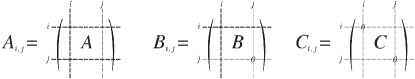
Figure 1: Figure Example.

Since $P_{G}^{i,j}(1)=|A_{G}|$, the polynomial $P_{G}^{i,j}(1)-|A_{G}|$ is divisible by $X-1$ and we obtain:

$$L_{G}^{i,j}(X)=\frac{P_{G}^{i,j}(1)-|A_{G}|}{X-1}=|A_{G}^{i,j}|X+\big{(}|A_{G}|-|C_{G}^{i,j}|\big{)};$$

this can be easily verified by using the equation

$$|A_{G}|-|C_{G}^{i,j}|-|A_{G}^{i,j}|=|B_{G}^{i,j}|+|B_{G}^{j,i}|.$$

Hence,

$$\mathfrak{A}_{G}=\big{|}\big{(}|A_{G}^{i,j}|\big{)}_{i,j=1}^{n}\big{|},\quad\mathfrak{C}_{G}=\big{|}\big{(}|C_{G}^{i,k}|\big{)}_{i,j=1}^{n}\big{|}$$

are graph isomorphisms (here and further in this work we set $n=|V|$ as the number of vertices of $G$).

Note that if $\mathfrak{A}_{G}\neq\mathfrak{A}_{G}^{\prime}$ or $\mathfrak{C}_{G}\neq\mathfrak{C}_{G}^{\prime}$, the graphs $G$ and $G^{\prime}$ are definitely not isomorphic. On the contrary, if $\mathfrak{A}_{G}=\mathfrak{A}_{G}^{\prime}$ and $\mathfrak{C}_{G}=\mathfrak{C}_{G}^{\prime}$, these two graphs are not proved to be equivalent. But if we regard $\big{(}|A_{G}^{i,j}|\big{)}_{i,j=1}^{n}$ and $\big{(}|C_{G}^{i,k}|\big{)}_{i,j=1}^{n}$ as the connection matrices for some weighted graphs, we can repeat the whole method recursively by setting $A_{G}=\big{(}|A_{G}^{i,j}|\big{)}_{i,j=1}^{n}$ and $A_{G^{\prime}}=\big{(}|A_{G^{\prime}}^{i,j}|\big{)}_{i,j=1}^{n}$.

We summarize the above ideas in the following algorithm.

Algorithm GraphIsomorphism

Input: connection matrices $A_{G}$ and $A_{G^{\prime}}$ of the graphs $G$ and $G^{\prime}$;
Repeat the following code twice

$\{$

compute the matrices $\big{(}|A_{G}^{i,j}|\big{)}_{i,j=1}^{n}$ and $\big{(}|A_{G^{\prime}}^{i,j}|\big{)}_{i,j=1}^{n}$;

If (the sets of entries of these matrices are not equal)

$G\not\cong G^{\prime}$ and stop;

else If($\mathfrak{A}_{G}\neq\mathfrak{A}_{G^{\prime}}$)

$G\not\cong G^{\prime}$ and stop;

else If($\mathfrak{C}_{G}\neq\mathfrak{C}_{G^{\prime}}$)

$G\not\cong G^{\prime}$ and stop;

Set $A_{G}=\big{(}|A_{G}^{i,j}|\big{)}_{i,j=1}^{n}$ and $A_{G^{\prime}}=\big{(}|A_{G^{\prime}}^{i,j}|\big{)}_{i,j=1}^{n}$;

$\}$

$G\cong G^{\prime}$

Obviously, the complexity of this method is $O(n^{5})$, but using the special methods (computation of the inverse matrix of $A_{G}$ in the case $\det(A_{G})\neq 0$ and using its symmetry) the upper bound can be reduced to $O(n^{4})$.

Another problem that arises during the computation is that the determinants

$$\big{|}\big{(}|A_{G}^{i,j}|\big{)}_{i,j=1}^{n}\big{|},\quad\big{|}\big{(}|A_{G}^{i,j}|\big{)}_{i,j=1}^{n}\big{|}$$

can become very large. In our computations, for the projective plane of order 16 with the $546\times 546$ connection matrix each determinant is 1086 decimal digits long (these computations were done using Wolfram Mathematica 8). This problem can be solved by the computations in different finite fields $\mathbb{Z}_{p_{l}}$, $D_{l}=|A_{G}^{i,j}|\mbox{\it\ mod }{p_{l}}$, $l\in\{1,\dots,k\}$, for coprime $p_{i}$s so that $P=p_{1}\cdot p_{2}\cdots p_{k}\geq|A_{G}^{i,j}|$. $|A_{G}^{i,j}|\in\mathbb{Z}_{P}$ can be restored due to the Chinese remainder theorem.

3 Computations and Experimental Results

As was shown in [1], the graph isomorphism problem can be solved efficiently for almost all graphs. The problems arise only considering special cases. The most efficient system known for today is Bredan McKay’s Nauty [12]. It is very efficient for most known hard graphs but has exponential running time on special family of graphs of bounded degree called Miyazaki graphs [14]. Besides this, most known systems have significant problems with the graphs originated from projective planes.

In this section, we show the experimental results after applying our methods to distinguish some types of hard graphs.

3.1 Fürer gadgets: Miyazaki graphs

Miyazaki graphs are special cases of a so called Cai–Fürer–Immerman construction based on Fürer gadgets ([5]). As an example consider a Miyazaki graph $M_{4}$ shown in Fig. 2(a).

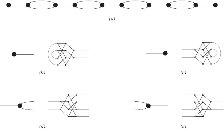
Figure 2: Example of a Miyazaki graph and its parts.

The bold circles represent special subgraphs shown in Fig. 2(b)–(e). One can easily extend this construction to a Miyazaki graph $M_{k}$ with arbitrary $k$.

Similarly, we define a twisted Miyazaki graph $MT_{4,2}$ that is identical with $M_{4}$ up to the 4th pair of bold knots: here two connections are twisted (cf. Fig. 3). One can easily generalize this construction to $MT_{n,k}$ with arbitrary $n,k\in\mathbb{N}$ and $k\leq n$.

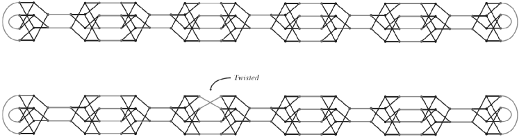
Figure 3: Miyazaki graph $M_{4}$ and twisted Miyazaki graph $MT_{4,2}$.

Distinguishing $M_{n}$ from $MT_{n,k}$ is a hard problem for graph isomorphism software and is widely used as a benchmark test. The following table shows the running times of our program on the Miyazaki graphs of different size.

Size	Matrix	Computation
$n$	Dimensions	Time in sec
10	$200\times 200$	9
15	$300\times 300$	26
20	$400\times 400$	60
25	$500\times 500$	133
30	$600\times 600$	1069
35	$700\times 700$	1940
40	$800\times 800$	5755

Remark. The determinants of the original connection matrices of Miyazaki graphs and their twisted counterparts are zero, so there is no fast computation possible using the inverse matrices. Therefore, we changed the corresponding connection matrices inserting 3 as diagonal elements. Due to this, for Miyazaki graphs of sizes $n\leq 25$ faster computation was available. This explains the sudden rise in computation time for size 30 and more.

3.2 Block designs: projective planes

A projective plane of order $n$ is an incidence structure on $n^{2}+n+1$ points, and equally many lines, (i.e., a triple $(P,L,I)$, where $P$, $L$ and $I$ are disjoint sets of the points, the lines and the incidence relation with $I\subset P\times L$ and $|P|=|L|=n^{2}+n+1$), such that:

1. for all pairs of distinct points $p,p^{\prime}\in P$, there is exactly one line $l\in L$ such that $(p,l)\in I$, $(p^{\prime},l)\in I$;

2. for all pairs of distinct lines $l,l^{\prime}\in L$, there is exactly one point $p\in P$ such that $(p,l)\in I$, $(p,l^{\prime})\in I$;

3. there are four points such that no line is incident with more than two of these points.

The smallest projective plain is the Fano plane of order $2$ shown in Fig. 4(a). It is also the only plane of this order.

We consider the corresponding incidence graphs of different projective plains and try to solve the graph isomorphism problem for them. The incidence graph of the Fano plane is shown in Fig. 4(b). In general, distinguishing projective planes of the same order by their incidence graphs poses a difficult challenge for graph isomorphism algorithms. The web page of Moorhouse [13] offers a collection of known projective planes.

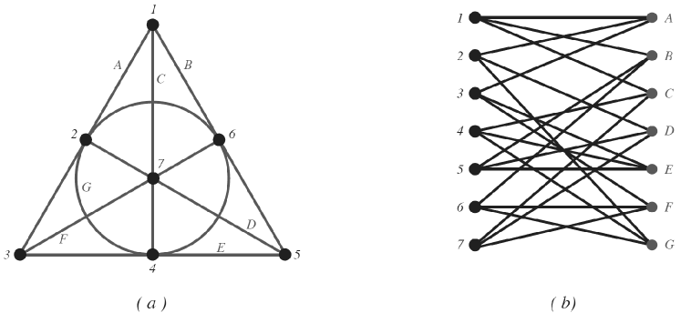
Figure 4: The least projective plane: the Fano plane.

Since the computation in Wolfram’s Mathematica 8 takes very long time for such large graphs, the algorithm was implemented in the C programming language. To calculate very large numbers while computing $\mathfrak{A}_{G}$ or $\mathfrak{C}_{G}$ the chinese remainder theorem was used. Each $d^{G}_{i,j,k}=|A_{G}^{i,j}|\mbox{\it\ mod }{p_{k}}$ was computed modulo a prime $43969\leq p_{k}\leq 44699$ ($l\in\{1,2,\dots,72\}$) and the result was calculated by the formula

$$|A_{G}^{i,j}|=\sum_{k=1}^{72}d^{G}_{i,j,k}m_{k}s_{k},$$

where $m_{k}=m/p_{k}$, $m=p_{1}\cdots p_{72}$, and $s_{k}=m_{k}^{-1}\mbox{\it\ mod }{p_{i}}$.

So, instead of very large numbers, we have to manipulate with lists of relatively small numbers: each $|A_{G}^{i,j}|$ corresponds to a list of 72 natural numbers that we denote by

$$H_{G}^{i,j,k}=\big{\{}d^{G}_{i,j,k}\mid 1\leq k\leq 72\big{\}}.$$

In fact, it suffices to compute each $|A_{G}^{i,j}|\mbox{\it\ mod }{p_{1}}$ (modulo one sufficiently large prime). If the sorted corresponding lists are differenent, $H_{G}^{i,j,1}\neq H_{G^{\prime}}^{i,j,1}$, where

$$H_{G}^{i,j,k}=\mbox{\it\ Sort }\Big{(}\big{\{}|A_{G}^{i,j}|\mbox{\it\ mod }{p_{k}}\mid 1\leq k\leq 72\big{\}}\Big{)},$$

we can be sure that the graphs $G$ and $G^{\prime}$ are not isomorphic, otherwise we obtain two weighted graphs $(d^{G}_{i,j,k})_{i,j=1}^{m}$ and $(d^{G^{\prime}}_{i,j,k})_{i,j=1}^{m}$ with $m=2(n^{2}+n+1)$, where $n$ is the order of the projective plane, and repeat the whole algorithm for them. If $H_{G}^{i,j,k}=H_{G^{\prime}}^{i,j,k}$ for each $1\leq k\leq 72$ in the second iteration, the graphs are conjectured to be isomorphic.

In general, if $H_{G}^{i,j,k}=H_{G^{\prime}}^{i,j,k}$ for each $1\leq k\leq 72$, we can consider the weighted graphs as above and proceed with the iteration, but we need a halting criteria to decide when the two graphs are isomorphic. In our experiments, the differences of most non-isomorphic graphs were discovered in the first iteration step, however for some projective planes two iterations were needed.

Order	No. of	Matrix	Iteration	Computation
$n$	planes	dimensions	steps	time in sec
9	4	$182\times 182$	2	63 $\cdot 2$=126
11	1	$266\times 266$	2	162$\cdot$2=324
13	1	$366\times 366$	2	467$\cdot$2=934
16	22	$546\times 546$	1	5460
25	193	$1302\times 1302$	1	52080

Note that in some cases (such as for $n=11$, $13$, $17$, $19$, or $23$) there is only one real projective plane, however it is self-dual.

For $n=27$, the determinants for the $1415\times 1415$ matrices were calculated on a parallel machine with 20 Intel Xeon 2.80 GHz CPUs. While the computations for basic graphs took relatively reasonable time, the computations for their duals lasted over twenty times as much for one iteration step (see the table below).

Andre	Hering	Sherk
$15584.9+89377.6$	$38125.7+9757.26$	$44448.8+9726.34$
104962.5	47882.96	54175.14
Andre dual	Hering dual	Sherk dual
944676	976157	964906

Flag 4	Flag 6
$35047.3+9771.57$	$34881+9773.86$
44818.87	44654.86
Flag 4 Dual	Flag 6 Dual
984884	1036820

4 Conclusions and Open Questions

In this paper, we have developed an $O(n^{5})$ polynomial-time algorithm that computes graph invariant for graphs with $n$ vertices. The main approach is based on random walks on graphs with the probability to stay in the actual node. Due to this, we generate a set of $n(n-1)/2$ quadratic polynomials of one variable. Comparing these sets we can distinguish different graphs. In some cases, two iterations of the algorithm are needed. The experimental results on some hard graphs (Miyazaki graphs as special Fürer gadgets and point-line incidence graphs of finite projective planes of higher degrees) show that our system can distinguish non-isomorphic graphs of this kind in reasonable time. It is a matter of further research to prove (or disprove) that the given method is a full graph invariant and to investigate the question why there are relative break-ins in the computational time for some point-line incidence graphs of dual finite projective planes of high order.

References

- [1] L. Babai, P. Erdös, S. M. Selkow. Random Graph Isomorphism. SIAM Journal on Computation, Vol. 9, 826 - 635 (1980)
- [2] Laszlo Babai, D. Yu. Grigoryev, and David M. Mount. Isomorphism of graphs with bounded eigenvalue multiplicity. In Proceedings of STOC, pages 310 - 324, 1982
- [3] R. Boppana, J. Hastad, and S. Zachos. Does co-NP have short interactive proofs? Inform. Process. Lett., 25 (1987), pp. 27 32.
- [4] S. R. Buss, Alogtime algorithms for tree isomorphism, comparison, and canonization. In Computational Logic and Proof Theory, Lecture Notes in Comput. Sci. 1289, Springer-Verlag, Berlin, 1997, pp. 18 33
- [5] Jin-Yi Cai, Martin Fürer, and Neil Immerman. An optimal lower bound on the number of variables for graph identification. Combinatorica, 12(4): 389 - 410, 1992.
- [6] I. S. Filotti and Jack N. Mayer. A polynomial-time algorithm for determining the isomorphism of graphs of fixed genus. In Proceedings of STOC, pages 236 - 243, 1980.
- [7] John E. Hopcroft and J. K. Wong. Linear time algorithm for isomorphism of planar graphs. In Proceedings of STOC, pages 310 - 324, 1974.
- [8] S. Lindell, A logspace algorithm for tree canonization. in Proceedings of the 24th Annual ACM Symposium on Theory of Computing, 1992, pp. 400 404
- [9] Eugene M. Luks. Isomorphism of graphs of bounded valence can be tested in polynomial time. Journal of Computer and System Sciences, 25(1):42 - 65, 1982.
- [10] E. Luks, Parallel algorithms for permutation groups and graph isomorphism. In Proceedings of the 27th IEEE Symposium on Foundations of Computer Science, 1986, pp. 292 302.
- [11] R. Mathon, A note on the graph isomorphism counting problem. Inform. Process. Lett., 8 (1979), pp. 131 132
- [12] McKay, B., The Nauty System: http://cs.anu.edu.au/~bdm/nauty
-
[13]
Eric Moorhouse.
Projective planes of small order.
http://www.uwyo.edu/moorhouse/pub/planes - [14] Miyazaki, T., The complexity of McKay’s canonical labeling algorithm: In Groups and computation, II, volume 28 of DIMACS Series in Discrete Mathematics and Theoretical Computer Science, American Mathematical Society, pages 239 - 256 (1995)
- [15] U. Schöning, Graph isomorphism is in the low hierarchy. J. Comput. System Sci., 37 (1988), pp. 312 323
- [16] Robert Endre Tarjan. A V 2 algorithm for determining isomorphism of planar graphs. Information Processing Letters, 1(1):32 - 34, 1971.