The Modified Direct Method: an Approach for Smoothing Planar and Surface Meshes

Abstract

The Modified Direct Method (MDM) is an iterative mesh smoothing method for smoothing planar and surface meshes, which is developed from the non-iterative smoothing method originated by Balendran1. . When smooth planar meshes, the performance of the MDM is effectively identical to that of Laplacian smoothing, for triangular and quadrilateral meshes; however, the MDM outperforms Laplacian smoothing for tri-quad meshes. When smooth surface meshes, for triangular, quadrilateral and quad-dominant mixed meshes, the mean quality(MQ) of all mesh elements always increases and the mean square error (MSE) decreases during smoothing; For tri-dominant mixed mesh, the quality of triangles always descends while that of quads ascends. Test examples show that the MDM is convergent for both planar and surface triangular, quadrilateral and tri-quad meshes.

1 Introduction

In finite element analysis it is important always to use high quality meshes: low quality meshes lead to unreliable results. A mesh that has been newly created usually needs to be improved before it can be used. This improvement can be made using either (1) mesh clear-up methods, which insert or delete nodes as well as change the connectivity of the mesh elements, or (2) mesh smoothing methods, which leave the element connectivity unchanged and instead reposition the mesh nodes. This paper is mainly concerned with smoothing methods.

There are numerous papers published concerning the topic of mesh smoothing. In this paper, we just refer some that are the most popular or representative of the state of the art for planar and surface meshes.

1.1 Related works

Mesh smoothing methods probably can be classified into four types: the geometry-based, the optimization-based, the physics-based and the combined. The geometry-based methods obtain new location of nodes by geometric rules, local optimization techniques or minimizing objective functions.

The most popular geometry-based smoothing methods is the Laplacian smoothing 13. , which repositions each node at the centroid of its neighboring nodes in one iteration. The popularity of this method comes from its simplicity and effectiveness. To improve the basic form of Laplacian smoothing, some smart, constrained or weighted variations have been proposed 9. ; 12. ; 29. .

Another simpler but more effective method is called angle-based approach 30. , in which new nodal locations are calculated by conforming specific angle ratios in the surrounding polygons. A geometric element transformation method (GETMe) 27. based on a simple geometric transformation can be applicable to elements bounded by polygons.

A projecting/smoothing method is performed for smoothing surface mesh by minimizing the mean ratio of all triangles sharing the free node8. . A novel method based on quadric surface fitting, vertex projecting, curvature estimating and mesh labeling is applied in biomedical modeling28. .

An effective variational method for smoothing surface and volume triangulations is proposed by Jiao X et al 16. , where the discrepancies between actual and target elements is reduced by minimizing two energy functions. Also, a general-purpose algorithm called the target-matrix paradigm is introduced in 18. , and can be applied to a wide variety of meshes.

Different from the geometry-based methods, in optimization-based ones, the smoothed position of all nodes is acquired by minimizing a given distortion metric. This series of methods is more expensive but can generate better results than most geometry-based ones especially at concave regions. Some literatures devoted on this topic include 3. ; 11. ; 22. ; 24. .

The physics-based smoothing methods are the techniques that smooth meshes based on physical processing21. , or by solving simple physics problems. Shimada 23. proposed a method which treats nodes as the center of bubbles and nodal locations are obtained by deforming bubbles with each other. A similar algorithm called pliant method is presented in 2. .

To improve performance, two or more basic methods can be combined into a hybrid approach. Some hybrid methods are the combination of Laplacian smoothing with optimization-based methods 4. ; 5. ; 10. .

In the aspect of computation, mesh smoothing methods can be either iterative or non-iterative. Most of them are iterative algorithms; a non-iterative method is proposed by Balendran 1. which is referred to here as the Direct Method (DM). The goal of the DM is simple – to make triangular elements as close to equilateral as possible and quadrilateral elements as close to square as possible – and it achieves this goal by generating and solving a set of optimization equations.

1.2 Our contribution

In this paper we introduce a smoothing method that has the same basic goal as the DM, but is iterative rather than non-iterative; we term this method the Modified Direct Method (MDM) which can be used to smooth both planar and surface meshes.

The main procedure of MDM for smoothing planar meshes is relatively simple: Firstly element stiffness matrices are created based on the type of elements. The modified forms of element stiffness matrices are simpler than those of DM. And then by assembling all element stiffness matrices, a system of Jacobi iteration equations can be formed, which is different from the optimization equations in DM. Finally, the smoothed nodal coordinates can be generated by solving the system of Jacobi iteration equations.

For smoothing surface meshes, the MDM becomes complex: Firstly to maintain features of original meshes, feature points are detected and then fixed as constrained nodes. Then a Jacobi iteration matrix which is similar to that in 2D is also assembled. Thirdly the relocated position of every node in each iteration is calculated according to the Jacobi iteration matrix, and then projected onto the original mesh to be smoothed position in current iteration. And finally, the required smoothed nodal coordinates can be obtained until the quality of smoothed mesh will not improve.

The paper is organized as follows. In Sect.2, we first give a brief description of the basics of the original DM. Then in Sect. 3, we show how the DM is modified and developed into the MDM for smoothing planar and surface meshes; also we introduce several key techniques such as features detection of the MDM for smoothing surface meshes. Finally we present some tests of the MDM and make a convergence analysis of the MDM for smoothing surface meshes, and summarize them in Sect.4.

2 The Direct Method (DM)

The optimization equations solved in the DM are generated by assembling element stiffness matrices into a global stiffness matrix. These element stiffness matrices are 6$\times$6 in size for planar triangular elements and 8$\times$8 in size for planar quadrilateral elements. The global stiffness matrix for a mesh with $n$ nodes is $2n\times 2n$ in size, irrespective of whether the elements are triangles or quadrilaterals.

2.1 Planar triangular mesh

The element stiffness matrix

Consider a triangular element ABC shown in Fig. 1. A^∗ is the position to which node A would have to be moved to make the element equilateral, assuming that nodes B and C were fixed; B^∗ is the position to which B would have to be moved assuming A and C were fixed; C^∗ is the position to which C would have to be moved assuming A and B were fixed. The coordinates of A^∗ are:

$$\left\{{{\begin{array}[]{*{20}l}{X_{A}^{*}=\dfrac{1}{2}(X_{B}+X_{C})+\dfrac{\sqrt{3}}{2}(Y_{B}-Y_{C})}\\ {Y_{A}^{*}=\dfrac{\sqrt{3}}{2}(-X_{B}+X_{C})+\dfrac{1}{2}(Y_{B}+Y_{C})}\\ \end{array}}}\right.$$ (1)

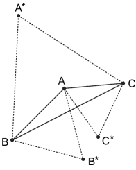
Figure 1: Triangular element ABC. A*, B*, C* are positions to which nodes would have to be moved singly in order to make ABC equilateral. See Eq. 3

These equations can be rewritten as:

$$\left\{{{\begin{array}[]{*{20}l}{2(X_{A}-X_{A}^{*})=(2X_{A}+0Y_{A})-(X_{B}+\sqrt{3}Y_{B})+(-X_{C}+\sqrt{3}Y_{C})}\\ {2(Y_{A}-Y_{A}^{*})=(0X_{A}+2Y_{A})+(\sqrt{3}X_{B}-Y_{B})-(\sqrt{3}X_{C}+Y_{C})}\\ \end{array}}}\right.$$ (2)

The coordinates of B^∗ and C^∗ are obtained in the same way. The coordinates of A, B, C, A^∗, B^∗ and C^∗ are related by the following equations:

$$\begin{bmatrix}2&0&{-1}&{-\sqrt{3}}&{-1}&{\sqrt{3}}\\ 0&2&{\sqrt{3}}&{-1}&{-\sqrt{3}}&{-1}\\ {-1}&{\sqrt{3}}&2&0&{-1}&{-\sqrt{3}}\\ {-\sqrt{3}}&{-1}&0&2&{\sqrt{3}}&{-1}\\ {-1}&{-\sqrt{3}}&{-1}&{\sqrt{3}}&2&0\\ {\sqrt{3}}&{-1}&{-\sqrt{3}}&{-1}&0&2\end{bmatrix}\begin{bmatrix}X_{A}\\ Y_{A}\\ X_{B}\\ Y_{B}\\ X_{C}\\ Y_{C}\end{bmatrix}=\begin{bmatrix}2(X_{A}-X_{A}^{*})\\ 2(Y_{A}-Y_{A}^{*})\\ 2(X_{B}-X_{B}^{*})\\ 2(Y_{B}-Y_{B}^{*})\\ 2(X_{C}-X_{C}^{*})\\ 2(Y_{C}-Y_{C}^{*})\end{bmatrix}$$ (3)

The left-hand matrix in Eq. 3 is termed the stiffness matrix of the planar triangular element.

The global stiffness matrix and the optimization equations

Now assume that ABC is part of a planar triangular mesh that has $n$ nodes. Each node of ABC – for instance node A – is then shared with several other elements, and A^∗ can be calculated for each of these. The final position of A – its optimal smoothed position – is obtained by averaging the separately calculated A^∗’s (Fig. 2). (This averaging process is effectively identical to that used in Laplacian smoothing, which explains why the test results obtained using Laplacian smoothing are identical to those obtained using MDM, for uniformly triangular and uniformly quadrilateral meshes – see Figs 4, 5.)

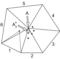
Figure 2: Node A belongs to 6 triangular elements. A* can be calculated for each element separately (black circles). Optimal smoothed position for A is the centroid of these, $A_{c}^{*}$(arrowed open circle)

The smoothed positions for the complete set of $n$ nodes are given by the equations:

$$\begin{bmatrix}{\alpha_{11}}&{\alpha_{12}}&{\alpha_{13}}&\cdots&{\alpha_{1(2n)}}\\ {\alpha_{21}}&{\alpha_{22}}&{\alpha_{23}}&\cdots&{\alpha_{2(2n)}}\\ {\alpha_{31}}&{\alpha_{32}}&{\alpha_{33}}&\cdots&{\alpha_{3(2n)}}\\ \vdots&\vdots&\vdots&\ddots&\vdots\\ {\alpha_{(2n)1}}&{\alpha_{(2n)2}}&{\alpha_{(2n)3}}&\cdots&{\alpha_{(2n)(2n)}}\\ \end{bmatrix}\begin{bmatrix}{X_{1}}\\ {Y_{1}}\\ {X_{2}}\\ \vdots\\ {Y_{n}}\end{bmatrix}=\begin{bmatrix}{e_{1}\cdot 2(X_{1}-X_{1}^{\ast})}\\ {e_{1}\cdot 2(Y_{1}-Y_{1}^{\ast})}\\ {e_{2}\cdot 2(X_{2}-X_{2}^{\ast})}\\ \vdots\\ {e_{n}\cdot 2(Y_{n}-Y_{n}^{\ast})}\end{bmatrix}$$ (4)

These equations are the optimization equations that need to be solved in the DM. The left-hand matrix – this is termed the global stiffness matrix – is created by assembling the individual element stiffness matrices according to the connectivity of the elements in the mesh concerned. The elements in the global stiffness matrix are obtained during this assembly process, and they will of course be different from mesh to mesh. $e_{i}(1\leq i\leq n)$is the number of elements in the mesh that share node $i$.

2.2 Planar quadrilateral mesh

The element stiffness matrix

Consider next a quadrilateral element ABCD shown in Fig. 3. A^∗ and C^∗ are the positions to which nodes A and C would have to be moved to make the element square, assuming B and D were fixed. The coordinates of A^∗ are:

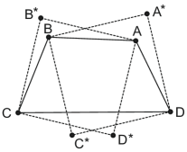
Figure 3: Quadrilateral element ABCD. A*, B*, C*, D* are positions to which diagonally opposite nodes would have to be moved to make ABCD square. See Eq.6

$$\left\{{{\begin{array}[]{*{20}l}{X_{A}^{*}=\dfrac{1}{2}(X_{B}+X_{D})+\dfrac{1}{2}(Y_{B}-Y_{D})}\\ {Y_{A}^{*}=\dfrac{1}{2}(-X_{B}+X_{D})+\dfrac{1}{2}(Y_{B}+Y_{D})}\\ \end{array}}}\right.$$ (5)

Similarly as that to triangular element, the coordinates of A, B, C, D, A^∗, B^∗, C^∗ and D^∗ are related by the following equations:

$$\begin{bmatrix}2&0&{-1}&{-1}&0&0&{-1}&1\\ 0&2&1&{-1}&0&0&{-1}&{-1}\\ {-1}&1&2&0&{-1}&{-1}&0&0\\ {-1}&{-1}&0&2&1&{-1}&0&0\\ 0&0&{-1}&1&2&0&{-1}&{-1}\\ 0&0&{-1}&{-1}&0&2&1&{-1}\\ {-1}&{-1}&0&0&{-1}&1&2&0\\ 1&{-1}&0&0&{-1}&{-1}&0&2\\ \end{bmatrix}\begin{bmatrix}{X_{A}}\\ {Y_{A}}\\ {X_{B}}\\ {Y_{B}}\\ {X_{C}}\\ {Y_{C}}\\ {X_{D}}\\ {Y_{D}}\\ \end{bmatrix}=\begin{bmatrix}{2(X_{A}-X_{A}^{\ast})}\\ {2(Y_{A}-Y_{A}^{\ast})}\\ {2(X_{B}-X_{B}^{\ast})}\\ {2(Y_{B}-Y_{B}^{\ast})}\\ {2(X_{C}-X_{C}^{\ast})}\\ {2(Y_{C}-Y_{C}^{\ast})}\\ {2(X_{D}-X_{D}^{\ast})}\\ {2(Y_{D}-Y_{D}^{\ast})}\\ \end{bmatrix}$$ (6)

The left-hand matrix in Eq. 6 is termed the stiffness matrix of the planar quadrilateral element.

The global stiffness matrix and the optimization equations

Now assume ABCD is part of a quadrilateral mesh that has $n$ nodes. As before, the global stiffness matrix is obtained by assembling the element stiffness matrices according to the connectivity of the elements in the mesh concerned. The optimization equations associated with this global stiffness matrix are identical in form to those for the triangular mesh (Eq. 4).

3 The Modified Direct Method (MDM)

The development of the MDM from the DM involves (1) the use of different element stiffness matrices, (2) the use of a Jacobian iteration matrix instead of a global stiffness matrix, and (3) the replacement of the optimization equations with iteration equations. The mathematical steps involved in this development are broadly similar for the triangular mesh, the quadrilateral mesh and the tri-quad mesh.

3.1 The element stiffness matrices

Triangular mesh

According to Eq. 1, the coordinates of A, B, C, A^∗, B^∗ and C^∗ are then related by the following equations:

$$\begin{bmatrix}0&0&{1/2}&{\sqrt{3}/2}&{1/2}&{-\sqrt{3}/2}\\ 0&0&{-\sqrt{3}/2}&{1/2}&{\sqrt{3}/2}&{1/2}\\ {1/2}&{-\sqrt{3}/2}&0&0&{1/2}&{\sqrt{3}/2}\\ {\sqrt{3}/2}&{1/2}&0&0&{-\sqrt{3}/2}&{1/2}\\ {1/2}&{\sqrt{3}/2}&{1/2}&{-\sqrt{3}/2}&0&0\\ {-\sqrt{3}/2}&{1/2}&{\sqrt{3}/2}&{1/2}&0&0\\ \end{bmatrix}\begin{bmatrix}{X_{A}}\\ {Y_{A}}\\ {X_{B}}\\ {Y_{B}}\\ {X_{C}}\\ {Y_{C}}\\ \end{bmatrix}=\begin{bmatrix}{X_{A}^{\ast}}\\ {Y_{A}^{\ast}}\\ {X_{B}^{\ast}}\\ {Y_{B}^{\ast}}\\ {X_{C}^{\ast}}\\ {Y_{C}^{\ast}}\\ \end{bmatrix}$$ (7)

These equations can also be rewritten as iteration equations:

$$\begin{bmatrix}0&0&{1/2}&{\sqrt{3}/2}&{1/2}&{-\sqrt{3}/2}\\ 0&0&{-\sqrt{3}/2}&{1/2}&{\sqrt{3}/2}&{1/2}\\ {1/2}&{-\sqrt{3}/2}&0&0&{1/2}&{\sqrt{3}/2}\\ {\sqrt{3}/2}&{1/2}&0&0&{-\sqrt{3}/2}&{1/2}\\ {1/2}&{\sqrt{3}/2}&{1/2}&{-\sqrt{3}/2}&0&0\\ {-\sqrt{3}/2}&{1/2}&{\sqrt{3}/2}&{1/2}&0&0\end{bmatrix}\begin{bmatrix}{X_{A}^{k}}\\ {Y_{A}^{k}}\\ {X_{B}^{k}}\\ {Y_{B}^{k}}\\ {X_{C}^{k}}\\ {Y_{C}^{k}}\\ \end{bmatrix}=\begin{bmatrix}{X_{A}^{k+1}}\\ {Y_{A}^{k+1}}\\ {X_{B}^{k+1}}\\ {Y_{B}^{k+1}}\\ {X_{C}^{k+1}}\\ {Y_{C}^{k+1}}\\ \end{bmatrix}$$ (8)

$X_{A}^{k}$ and $Y_{A}^{k}$ are the coordinates of node A at step $k$, and $X_{A}^{k+1}$ and $Y_{A}^{k+1}$ are the coordinates at step $k$+1; the notation for nodes B and C is similar. The left-hand matrix in Eq.8 is also the element stiffness matrix for a planar triangular element, but it is simpler in form to that used in the DM (Eq.3).

In Cartesian coordinates, the coordinates of a vertex x, y and z are equivalent and can be cycled in sequence: $X\to Y,Y\to Z,Z\to X$. Hence, we easily extend the stiffness matrix (Eq.8) for a planar triangular element to a surface one in 3D (Eq.9).

$$\begin{bmatrix}0&0&0&{1/2}&{\sqrt{3}/2}&{-\sqrt{3}/2}&{1/2}&{-\sqrt{3}/2}&{\sqrt{3}/2}\\ 0&0&0&{-\sqrt{3}/2}&{1/2}&{\sqrt{3}/2}&{\sqrt{3}/2}&{1/2}&{-\sqrt{3}/2}\\ 0&0&0&{\sqrt{3}/2}&{-\sqrt{3}/2}&{1/2}&{-\sqrt{3}/2}&{\sqrt{3}/2}&{1/2}\\ {1/2}&{-\sqrt{3}/2}&{\sqrt{3}/2}&0&0&0&{1/2}&{\sqrt{3}/2}&{-\sqrt{3}/2}\\ {\sqrt{3}/2}&{1/2}&{-\sqrt{3}/2}&0&0&0&{-\sqrt{3}/2}&{1/2}&{\sqrt{3}/2}\\ {-\sqrt{3}/2}&{\sqrt{3}/2}&{1/2}&0&0&0&{\sqrt{3}/2}&{-\sqrt{3}/2}&{1/2}\\ {1/2}&{\sqrt{3}/2}&{-\sqrt{3}/2}&{1/2}&{-\sqrt{3}/2}&{\sqrt{3}/2}&0&0&0\\ {-\sqrt{3}/2}&{1/2}&{\sqrt{3}/2}&{\sqrt{3}/2}&{1/2}&{-\sqrt{3}/2}&0&0&0\\ {\sqrt{3}/2}&{-\sqrt{3}/2}&{1/2}&{-\sqrt{3}/2}&{\sqrt{3}/2}&{1/2}&0&0&0\\ \end{bmatrix}$$ (9)

Quadrilateral mesh

According to Eq.5, The coordinates of A, B, C, D, A^∗, B^∗, C^∗ and D^∗ can also be rewritten as iteration equations:

$$\begin{bmatrix}0&0&{1/2}&{1/2}&0&0&{1/2}&{-1/2}\\ 0&0&{-1/2}&{1/2}&0&0&{1/2}&{1/2}\\ {1/2}&{-1/2}&0&0&{1/2}&{1/2}&0&0\\ {1/2}&{1/2}&0&0&{-1/2}&{1/2}&0&0\\ 0&0&{1/2}&{-1/2}&0&0&{1/2}&{1/2}\\ 0&0&{1/2}&{1/2}&0&0&{-1/2}&{1/2}\\ {1/2}&{1/2}&0&0&{1/2}&{-1/2}&0&0\\ {-1/2}&{1/2}&0&0&{1/2}&{1/2}&0&0\\ \end{bmatrix}\begin{bmatrix}{X_{A}^{k}}\\ {Y_{A}^{k}}\\ {X_{B}^{k}}\\ {Y_{B}^{k}}\\ {X_{C}^{k}}\\ {Y_{C}^{k}}\\ {X_{D}^{k}}\\ {Y_{D}^{k}}\\ \end{bmatrix}=\begin{bmatrix}{X_{A}^{k+1}}\\ {Y_{A}^{k+1}}\\ {X_{B}^{k+1}}\\ {Y_{B}^{k+1}}\\ {X_{C}^{k+1}}\\ {Y_{C}^{k+1}}\\ {X_{D}^{k+1}}\\ {Y_{D}^{k+1}}\\ \end{bmatrix}$$ (10)

$$\setcounter{MaxMatrixCols}{12}\begin{bmatrix}0&0&0&{1/2}&{1/2}&{-1/2}&0&0&0&{1/2}&{-1/2}&{1/2}\\ 0&0&0&{-1/2}&{1/2}&{1/2}&0&0&0&{1/2}&{1/2}&{-1/2}\\ 0&0&0&{1/2}&{-1/2}&{1/2}&0&0&0&{-1/2}&{1/2}&{1/2}\\ {1/2}&{-1/2}&{1/2}&0&0&0&{1/2}&{1/2}&{-1/2}&0&0&0\\ {1/2}&{1/2}&{-1/2}&0&0&0&{-1/2}&{1/2}&{1/2}&0&0&0\\ {-1/2}&{1/2}&{1/2}&0&0&0&{1/2}&{-1/2}&{1/2}&0&0&0\\ 0&0&0&{1/2}&{-1/2}&{1/2}&0&0&0&{1/2}&{1/2}&{-1/2}\\ 0&0&0&{1/2}&{1/2}&{-1/2}&0&0&0&{-1/2}&{1/2}&{1/2}\\ 0&0&0&{-1/2}&{1/2}&{1/2}&0&0&0&{1/2}&{-1/2}&{1/2}\\ {1/2}&{1/2}&{-1/2}&0&0&0&{1/2}&{-1/2}&{1/2}&0&0&0\\ {-1/2}&{1/2}&{1/2}&0&0&0&{1/2}&{1/2}&{-1/2}&0&0&0\\ {1/2}&{-1/2}&{1/2}&0&0&0&{-1/2}&{1/2}&{1/2}&0&0&0\\ \end{bmatrix}$$ (11)

The left-hand matrix is also the element stiffness matrix for a planar quadrilateral element, but it is simpler in form to that used in the DM (Eq.6). Similarly, the 2D version of stiffness matrix for a planar quadrilateral element (Eq.10) can be extended into 3D version (Eq.11).

Tri${-}$quad mesh

The element stiffness matrices used in a tri-quad mesh are those already given for the triangular and quadrilateral meshes (Eq.8, 9, 10, 11). Which of these is used for a particular element in a tri-quad mesh depends only on that element’s type.

3.2 The MDM for smoothing planar meshes

Just as in the DM, the element stiffness matrices can be assembled into a global matrix, also of size $2n\times 2n$ for a mesh of $n$ nodes. This Jacobi iteration matrix has several forms, the one shown in Eq.12 is the most efficient computationally. Therefore it is the one that will need to be solved iteratively, starting with the original node coordinates at step 0 and continuing until no node needs to be moved by more than the given tolerance distance.

$$D\cdot\left\{\begin{bmatrix}{\alpha_{11}}&{\alpha_{12}}&{\alpha_{13}}&\cdots&{\alpha_{1(2n)}}\\ {\alpha_{21}}&{\alpha_{22}}&{\alpha_{23}}&\cdots&{\alpha_{2(2n)}}\\ {\alpha_{31}}&{\alpha_{32}}&{\alpha_{33}}&\cdots&{\alpha_{3(2n)}}\\ \vdots&\vdots&\vdots&\ddots&\vdots\\ {\alpha_{(2n)1}}&{\alpha_{(2n)2}}&{\alpha_{(2n)3}}&\cdots&{\alpha_{(2n)(2n)}}\\ \end{bmatrix}\begin{bmatrix}{X_{1}^{k}}\\ {Y_{1}^{k}}\\ {X_{2}^{k}}\\ \vdots\\ {Y_{n}^{k}}\\ \end{bmatrix}\right\}=\begin{bmatrix}{X_{1}^{k+1}}\\ {Y_{1}^{k+1}}\\ {X_{2}^{k+1}}\\ \vdots\\ {Y_{n}^{k+1}}\\ \end{bmatrix}$$ (12)

, where$D=diag(1/e{}_{1},\mbox{ }1/e_{1},\mbox{ }1/e_{2},\mbox{ }1/e_{2},\mbox{ }\cdots,\mbox{ }\cdots,\mbox{ }1/e_{n},\mbox{ }1/e_{n})$

The algorithm for implementing the MDM in 2D has three basic steps: (1) Search for elements that share a node, for each node; (2) Assemble of the element stiffness matrices into the iteration matrix; (3) Solve of the iteration equations until the tolerance distance is reached.

3.3 The MDM for smoothing surface meshes

When smooth surface meshes, it is necessary to keep the features of original meshes. Many features preservation approaches have been proposed7. ; 15. ; 17. . A popular methods is to classify all the nodes of a mesh into four types: boundary, corner, ridges and smooth nodes; and then boundary nodes and corner nodes are fixed while smooth node can be adjusted on the whole mesh and ridge nodes can only be relocated along the ridges.

In order to preserve features, we firstly detect the corner nodes and ridge nodes via Jiao’s approach 15. , and fix them as constrained nodes together with the boundary nodes although the ridge nodes can be moved along ridges; and then after obtaining the relocated positions based on the Jacobi iteration matrix, we project the these new nodes onto the original mesh to get the mapped ones which are still the candidates of the resulting nodes in this iteration; and thirdly, we check whether there exists inverted elements in the incident faces of the mapped node. If does, recover it; otherwise, update the target node with the mapped position(Algorithm.1).

Since the MDM is an iterative smoothing algorithm, we have to conduct some indicators to judge when the meshes are smoothed enough and then end the iteration. We adopt two mesh quality indicators, the mean quality of mesh (MQ) and mean square error (MSE) of all elements, to show target meshes are smoothed enough and iterations can break. This can be presented as:

$$\left\{\begin{array}[]{r@{,\quad}l}{if}\left\{\begin{array}[]{c}{\mbox{MQ}^{k+1}-\mbox{MQ}^{k}}<\varepsilon_{mq}\\ {\mbox{MSE}^{k+1}-\mbox{MSE}^{k}}<\varepsilon_{mse}\end{array}\right.&\mbox{stop}\\ {otherwise}&\mbox{continue to iterate}\end{array}\right.$$

, where $\varepsilon_{mq}$ and $\varepsilon_{mse}$ are two user-specified thresholds. Noticeably, the above criteria only works when there are no inverted elements.

Algorithm 1 The MDM for smoothing surface meshes

1:  Search all incident faces $F(v_{i})$ for each node $v_{i}$;

2:  Assemble the $3n\times 3n$ Jacobi iteration matrix ${\rm{\bf B}}=(b_{ij})_{0\leq i<3n,0\leq j<3n}$;

3:  while iteration not converge do

4:     Estimate or update normal at each node $v_{i}$

5:     for each node $v_{i}$ do

6:        if $v_{i}$ is not constrained then

7:           Calculate the relocated node $v_{i}^{new}$ based on ${\rm{\bf B}}$:

8:           Project $v_{i}^{new}$onto $F(v_{i})$ to obtain the mapped node $v_{i}^{map}$;

9:           Check inverted element in $F(v_{i}^{map})$. If exists, recover $\mbox{ }v_{i}^{map}\leftarrow v_{i}$

10:     Update all nodes: $v_{i}\mbox{ }\leftarrow v_{i}^{map}$

Normal of vertices

The direction of each vertex is closely related to its incident faces, for that the normal of each vertex is nearly vertical to the normal of any face of its incident elements. Therefore, the unit normal of each faces in a mesh should be calculated firstly by computing the planar equation of every face. Suppose there are $m$ faces shares the vertex $v$, and the normal of $v$ can be obtained by solving the following $m\times 3$ linear equations Nx=1, where ${\rm{\bf N}}$ is a $m\times 3$ matrix whose $i^{th}$ row is the unit normal of the $i^{th}$ incident face of the vertex $v$, and ${\rm{\bf 1}}=(1,1,\mbox{...,1})$ is a vector of length $m$. Since ${\rm{\bf N}}$ may be over- or under-determined, the solution is in least squares sense and can be solved by the singular value decomposition (SVD).

Identifying points

We adopt Jiao’s algorithm 15. to detect features based on eigenvalues analysis of a symmetric positive semi-definite matrix ${\rm{\bf A}}$: ${\rm{\bf A}}={\rm{\bf N}}^{T}{\rm{\bf WN}}$, where ${\rm{\bf N}}$ is a $m\times 3$ matrix we denote in above section, and ${\rm{\bf W}}$ be a $m\times m$ diagonal matrix with $W_{ii}$ equal to the weight. If users do not consider the weights, ${\rm{\bf W}}$ can be ignored and ${\rm{\bf A}}$ is then simplified as ${\rm{\bf N}}^{T}{\rm{\bf N}}$. Let $\lambda_{1}$, $\lambda_{2}$ and $\lambda_{3}$ ($\lambda_{1}\geq\lambda_{2}\geq\lambda_{3})$ be the three eigenvalues of ${\rm{\bf A}}$. The relative sizes of the eigenvalues $\lambda_{i}$ of ${\rm{\bf A}}$ are closely related to the local flatness at a vertex. In general, ${\rm{\bf A}}$ has three large eigenvalues at a corner, two large ones at a ridge, and one large one at a smooth point. Hence, the corners and ridges can be recognized by comparing $\lambda_{3}/\lambda_{1}$ and $\lambda_{2}/\lambda_{1}$ against some thresholds: $\mbox{if }\lambda_{3}/\lambda_{1}\geq\chi_{c},$ $v\mbox{ is at corner};$ $\mbox{if }\lambda_{2}/\lambda_{1}\geq\chi_{r},$ $v\mbox{ is on a ridge}$ , where $\chi_{c}$ and $\chi_{r}$ are two given thresholds.

Projecting

After relocating position in an iteration step, smooth node will be projected onto its incident faces of the original mesh alone the updated normal. Since that, we just project the relocated point onto its last incident faces (neighborhood), there maybe not exists a mapped point on the original mesh inside the neighborhood of the above node. Thus, let $k$ be the number of mapped points on the incident faces, then we have: (1) if $k=0$, ignore the relocated position and recover its last coordinates; (2) if $k=1$, adopt the only mapped point as the new position; (3) if $k>1$, select the nearest mapped point to the relocated position as the new position.

4 Test applications of the MDM

4.1 Mesh quality

The simplest way to measure mesh quality is to calculate distortion values for each of the mesh elements. The distortion value for a triangular element should measure how close that triangle is to equilateral. One appropriate measure, $\alpha$, was proposed by Lee and Lo20. . For the triangle ABC shown in Fig.1:

$$\alpha=2\sqrt{3}\frac{\left\|{\mbox{CA}\times\mbox{CB}}\right\|}{\left\|{\mbox{CA}}\right\|^{2}+\left\|{\mbox{AB}}\right\|^{2}+\left\|{\mbox{BC}}\right\|^{2}}$$

The value of $\alpha$ lies between 0 and 1; $\alpha$ = 0 when A, B and C are collinear; $\alpha$ = 1 when ABC is equilateral.

The distortion value for a quadrilateral element should measure how close that quadrilateral is to square. In this paper we use the measure $\lambda$ proposed by Hua 14. ; this applies only to convex quadrilaterals. For the quadrilateral ABCD shown in Fig.3:

$$\lambda=2\sqrt[4]{\frac{\left\|{\mbox{AB}\times\mbox{AD}}\right\|\cdot\left\|{\mbox{BC}\times\mbox{BA}}\right\|\cdot\left\|{\mbox{CD}\times\mbox{CB}}\right\|\cdot\left\|{\mbox{DA}\times\mbox{DC}}\right\|}{(\left\|{\mbox{AB}}\right\|^{2}+\left\|{\mbox{AD}}\right\|^{2})(\left\|{\mbox{BC}}\right\|^{2}+\left\|{\mbox{BA}}\right\|^{2})(\left\|{\mbox{CD}}\right\|^{2}+\left\|{\mbox{CB}}\right\|^{2})(\left\|{\mbox{DA}}\right\|^{2}+\left\|{\mbox{DC}}\right\|^{2})}}$$

The value of $\lambda$ lies between 0 and 1; $\lambda$ = 0 when any three nodes are collinear, i.e., when ABCD is in fact a triangle; $\lambda$ = 1 when ABCD is square.

4.2 The test applications

For smoothing planar meshes, a number of test meshes were created and smoothed (Figs. 4, 5, 6). The mesh quality results for tri-quad meshes before and after smoothing are given in Tables 1. For smoothing surface meshes, a tri and a quad surface mesh are created by planar triangulations19. ; 20. ; 25. and then interpolated to surface (Fig.8).

Table 1: Smoothing for planar tri-quad meshes(T: tri; Q: quad)

	T-dominant				Q-dominant
	T-MQ	T-MSE	Q-MQ	Q-MSE	T-MQ	T-MSE	Q-MQ	Q-MSE
Original	0.8688	0.1188	0.8211	0.0713	0.9079	0.1243	0.9194	0.0739
LS	0.8756	0.1083	0.8464	0.0571	0.9064	0.0936	0.9554	0.0568
MDM	0.8794	0.1083	0.8306	0.0583	0.9394	0.0737	0.9576	0.0568

A tri-dominant mixed mesh is generated by dividing each sliver triangle and its neighbors in the original triangular mesh into a smaller triangle and a quadrilateral (Fig.8(e)). Another quad-dominant mixed mesh is created by pairing triangles in 2D and then interpolating (Fig.8(g)).

(a) Original tri mesh

(b) Smoothed by LS/MDM

Figure 4: Smoothing for planar triangular mesh

The smoothed surface meshes are shown in Fig.8. The user-specified thresholds $\varepsilon_{mq}$ and $\varepsilon_{mse}$ are set as 10^-6, 10^-4, 10^-5 and 10^-4 for triangular, quadrilateral, tri-dominant and quad-dominant meshes, respectively. And correspondingly, the MDM converges at the steps 43, 56, 33 and 13. The mesh quality results before and after smoothing are given in Table 2.

(a) Original quad mesh

(b) Smoothed by LS/MDM

Figure 5: Smoothing for planar quadrilateral mesh

4.3 Convergence analysis

In this section, we analyze the convergence of the MDM. When smooth the planar meshes, test examples show that the MDM does converge. We have not given the mathematical proof for it in theory. For smoothing surface meshes, the MDM is much more complicated. As mentioned above, the mean quality of mesh (MQ) and mean square error (MSE) of element qualities are used to indicate the quality of whole mesh, we can calculate and compare the two indicators in increasing smoothing iterations to analyze the converge.

(a) Tri-dominant mesh

(b) Smoothed by LS

(c) Smoothed by MDM

(d) Quad-dominant mesh

(e) Smoothed by LS

(f) Smoothed by MDM

Figure 6: Smoothing for planar tri-quad meshes

The triangular surface (Fig.8(a)) is smoothed by MDM in 20, 40, 60, 80 and 100 iterations. The MQ and MSE of smoothed meshes in different iteration stages are listed in Table 2. And corresponding scatter diagrams are drawn in Fig. 7(a) and 7(b). It is clear that the mean quality of mesh ascends while MSE descends during increasing iterations. The quadrilateral mesh is smoothed by MDM in 10, 20, 30, 40 and 50 iterations. From Table 2 and Fig. 7(c) and 7(d), we can also receive the same conclusions as that of triangular mesh. Similarly, the tri-dominant mixed mesh is smoothed in 10, 20, 30, 40 and 50 iterations(Table 2, Fig. 7(e) and 7(f)), and the quad-dominant mixed mesh is smoothed in 5, 10, 15, 20 and 25 iterations(Table 2).

According to the scatter diagrams of MQ and MSE, we can learn that: for both triangular and quadrilateral surface meshes, the MQ always increases and the MSE decreases during smoothing. But the magnitude and rate of change are becoming smaller and smaller. Thus, we may in theory receive the conclusion that the smoothing iterations will converge after some steps. This can be also concluded for quad-dominant mixed mesh.

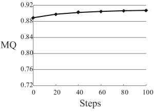
(a) MQs of smoothing tri mesh

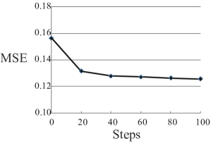
(b) MSEs of smoothing tri mesh

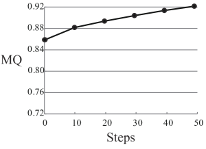
(c) MQs of smoothing quad mesh

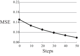
(d) MSEs of smoothing quad mesh

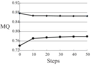
(e) MQs of smoothing tri-domi. mesh

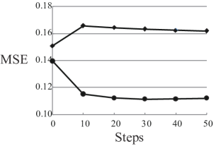
(f) MSEs of smoothing tri-domi. mesh

Figure 7: Mean quality(MQ) and mean square error of quality(MSE) when smooth surface triangular, quadrilateral and tri-domi. meshes. $\blacklozenge$:triangles, $\bullet$:quadrilterals

For the tri-dominant mixed mesh, the quality of triangles always decreases while that of quads increases. Noticeably, in beginning iteration steps, both of the above qualities change dramatically. Different from the mean qualities, the MSE is much more complex: the MSE of triangles significantly ascends in beginning steps, and then descends stably; the magnitude and rate of change are becoming smaller and smaller. The MSE of quadrilaterals seems to always decline, but obviously, there is an inflection point at steps 30(the MSEs at both steps 20 and steps 40 are bigger than that at steps 30); hence, there must be a convergence point around steps 30. Our tests (Table 2) proves the above conclusion: the MDM converges at steps 33 when the thresholds $\varepsilon_{mq}$ and $\varepsilon_{mse}$ are set as 10^-5. In Table 2, each stage includes 5, 10 or 20 steps.

Table 2: Qualities for smoothing surface meshes in increasing iteration steps

Meshes		Indicator	Stage 0	Stage 1	Stage 2	Stage 3	Stage 4	Stage 5
Tri mesh		MQ	0.8891	0.8980	0.9026	0.9049	0.9067	0.9073
		MSE	0.1565	0.1317	0.1281	0.1272	0.1264	0.1257
Quad mesh		MQ	0.8592	0.8814	0.8929	0.9027	0.9122	0.9198
		MSE	0.1466	0.1237	0.1088	0.0973	0.0874	0.0785
Tri of tri-domi.		MQ	0.8769	0.8672	0.8663	0.8660	0.8659	0.8658
		MSE	0.1509	0.1657	0.1644	0.1633	0.1625	0.1619
Quad of tri-domi.		MQ	0.7406	0.7711	0.7750	0.7772	0.7785	0.7792
		MSE	0.1397	0.1153	0.1123	0.1115	0.1116	0.1122
Tri of quad-domi.		MQ	0.9187	0.9417	0.9435	0.9449	0.9466	0.9481
		MSE	0.1066	0.0884	0.0839	0.0813	0.0777	0.0747
Quad of quad-domi.		MQ	0.8220	0.8625	0.8721	0.8788	0.8842	0.8887
		MSE	0.1432	0.1323	0.1235	0.1162	0.1102	0.1048

4.4 Tests assessment and summary

1) For the two topologically uniform planar meshes, i.e., the meshes with the same type of element throughout, there is effectively no difference between Laplacian smoothing and MDM. (This was referred to earlier, in the description of the original DM.) Both these methods give smoothed meshes that are markedly better than the original unsmoothed meshes.

2) For the triangular elements in the planar tri-dominant mixed mesh, the MDM outperforms Laplacian smoothing while for the quadrilateral elements, the reverse is true (Table 1). However, for planar quad-dominant mixed mesh, the MDM perfectly outperforms Laplacian smoothing for both triangular and quadrilateral elements.

3) For triangular, quadrilateral and quad-dominant mixed surface meshes, the MQ always increases and the MSE decreases in increasing iterations. For tri-dominant mixed mesh, the quality of triangles always descends while that of quads ascends.

4) Test examples shows that the MDM is convergent for both planar and surface triangular, quadrilateral and tri-quad meshes.

5) There are some ‘sharp’ vertices in the smoothed surface meshes. One of the probable cause is that both ridge and corner vertices are strictly fixed; the other possibly is to project relocated position onto the original meshes rather than an uniform underlying surface or a local parametric curve or surface.

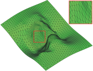
(a) Original triangular mesh

(b) Smoothed by MDM

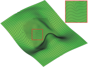
(c) Original quadrilateral mesh

(d) Smoothed by MDM

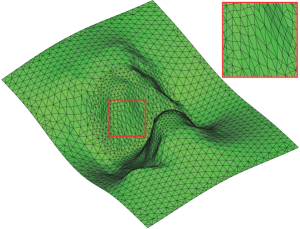
(e) Original tri-dominant mesh

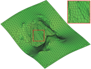
(f) Smoothed by MDM

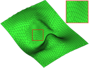
(g) Original quad-dominant mesh

(h) Smoothed by MDM

Figure 8: Smoothing surface meshes by MDM

- (1) Balendran B (1999) A direct smoothing method for surface meshes. In: Proceedings of 8th international meshing roundtable, pp 189–193
- (2) Bossen FJ, Heckbert PS (1996) A pliant method for anisotropic mesh generation. In: Proceedings of 5th international meshing roundtable, pp 63–74
- (3) Branets LV (2005) A variational grid optimization method based on a local cell quality metric. Ph.D. thesis, University of Texas at Austin
- (4) Canann SA, Tristano JR, Staten ML (1998) An approach to combined Laplacian and optimization -based smoothing for triangular, quadrilateral, and quad-dominant meshes. In: Proceedings of 7th international meshing roundtable, pp 479–494
- (5) Chen Z, Tristano JR, Kwok W (2003) Combined Laplacian and optimization-based smoothing for quadratic mixed surface meshes. In: Proceedings of 12th international meshing roundtable, pp 361–370
- (6) Escobar JM, Montero G, Montenegro R, Rodriguez E (2006) An algebraic method for smoothing surface triangulations on a local parametric space. Int J Numer Methods Eng 66 740-760.
- (7) Escobar JM, Montenegro R, Rodr’guez E, Montero G (2011) Simultaneous aligning and smoothing of surface triangulations. Eng Comput 27:17–29
- (8) Field DA (1988) Laplacian smoothing and Delaunay triangulation. Commun Appl Numer Methods 4:709–712
- (9) Freitag LA (1997) On combining Laplacian and optimization-based mesh smoothing techniques. AMD trends in unstructured mesh generation. ASME 220:37–43
- (10) Freitag L, Jones M, Plassmann P(1995) An efficient parallel algorithm for mesh smoothing. In: Proceedings of 4th international meshing roundtable, pp 47–58
- (11) Hansbo P (1995) Generalized Laplacian smoothing of unstructured grids. Commun Numer Methods Eng 11:455–464
- (12) Herrman LR (1976) Laplacian-isoparametric grid generation scheme. J Eng Mech EM5: 749–756
- (13) Hua L (1995) Automatic generation of quadrilateral mesh for arbitrary planar domains. Ph.D. thesis, Research Institute of Engineering Mechanics, Dalian University of Technology, China
- (14) Jiao X (2007) Volume and Feature Preservation in Surface Mesh Optimization. In: Proceedings of 17th international meshing roundtable, pp 315–332
- (15) Jiao X, Wang D, Zha H(2011). Simple and effective variational optimization of surface and volume triangulations. Eng Comput 27:81–94
- (16) Knupp PM (2000) Achieving finite element mesh quality via optimization of the Jacobian matrix norm and associated quan-tities. part I: a framework for surface mesh optimization. Int J Numer Methods Eng 48:401–420
- (17) Knupp PM(2010) Introducing the target-matrix paradigm for mesh optimization via node-movement. In: Proceedings of 19th international meshing roundtable, pp 67–83
- (18) Lawson CL (1977) Software for C1 surface interpolation. In: Rice JR (ed) Mathematical Software III. Academic Press, New York, pp 161–194
- (19) Lee CK, Lo SH (1994) A new scheme for the generation of a graded quadrilateral mesh. Comp Struct 52 (5): 847–857
- (20) Lohner R, Morgan K, Zienkiewicz OC (1986) Adaptive grid refinement for compressible Euler equations. In: Babuska I et al (eds) Accuracy estimates and adaptive refinements in finite element computations. Wiley, pp 281–297
- (21) Parthasarathy VN, Kodiyalam S (1991) A constrained optimization approach to finite element mesh smoothing. Finite Elem Anal Des 9:309–320
- (22) Shimada K (1997) Anisotropic triangular meshing of parametric surfaces via close packing of ellipsoidal bubbles. In: Proceedings of 6th international meshing roundtable, pp 375–390
- (23) Shivanna K, Grosland N, Magnotta V(2010) An analytical framework for quadrilateral surface mesh improvement with an underlying triangulated surface definition. In: Proceedings of 19th international meshing roundtable, pp 85–102
- (24) Tipper JC (1990) A straightforward iterative algorithm for the planar Voronoi diagram. Inf Proc Lett 14: 155–160
- (25) Vartziotis D, Wipper J(2009) The geometric element transformation method for mixed mesh smoothing. Eng Comput 25:287–301
- (26) Wang J, Yu Z(2009) A novel method for surface mesh smoothing: applications in biomedical modeling. In: Proceedings of 18th international meshing roundtable, pp 195–210
- (27) Zhihong M, Lizhuang M, Mingxi Z, Zhong L (2006) A modified Laplacian smoothing approach with mesh saliency. LNCS 4073:105–113
- (28) Zhou T, Shimada K (2000) An angle-based approach to two-dimensional mesh smoothing. In: Proceedings of 9th international meshing roundtable, pp 373–384