Large nuclear spin polarization in gate-defined quantum dots using a single-domain nanomagnet

Abstract

The electron-nuclei (hyperfine) interaction is central to spin qubits in solid state systems. It can be a severe decoherence source but also allows dynamic access to the nuclear spin states. We study a double quantum dot exposed to an on-chip single-domain nanomagnet and show that its inhomogeneous magnetic field crucially modifies the complex nuclear spin dynamics such that the Overhauser field tends to compensate external magnetic fields. This turns out to be beneficial for polarizing the nuclear spin ensemble. We reach a nuclear spin polarization of $\simeq$50\text{\,}\mathrm{\char 37\relax}$$, unrivaled in lateral dots, and explain our manipulation technique using a comprehensive rate equation model.

The hyperfine interaction (HFI) between few electrons and a bath of nuclear spins induces a complex quantum many-body dynamics which has been studied in a variety of systems including phosphorus donors in silicon Kane (1998), nitrogen vacancy centers in diamond Jelezko and Wrachtrup (2006), quantum Hall systems Kou et al. (2010), and semiconductor-based quantum dots, both optically Urbaszek et al. (2012) and in transport Schliemann et al. (2003); Fischer et al. (2009). In GaAs double quantum dots (DQDs), each electron interacts with $\sim$$10^{6}$ nuclear spins, which fluctuate thermally even at cryogenic temperatures. Their HFI causes electron spin decoherence Yao et al. (2006); Fischer et al. (2009); Cywinski et al. (2009); Bluhm et al. (2011), but it also offers a means to control the nuclear spins dynamically Laird et al. (2007); Petta et al. (2008); Foletti et al. (2009); Reilly et al. (2010). As has been proposed Burkard et al. (1999); Klauser et al. (2006); Rudner and Levitov (2007); Danon and Nazarov (2008) and demonstrated Latta et al. (2009); Vink et al. (2009); Danon et al. (2009), nuclear spin manipulation facilitates nuclear state preparation, which can enhance spin coherence times Bluhm et al. (2010); Sun et al. (2012). Nuclear spin manipulation has also motivated theoretical proposals Taylor et al. (2003); Kurucz et al. (2009) and experimental realizations Maurer et al. (2012); Steger et al. (2012) of nuclear spins as quantum memory.

Here, we present a novel nuclear spin manipulation technique. We couple a DQD with a single-domain nanomagnet whose inhomogeneous magnetic field does not depend on external fields. This allows measurements in a new regime, which will increase our fundamental understanding and control of the coupled electron-nuclei system common to a variety of platforms. As an example, we demonstrate unusually strong dynamic nuclear spin polarization (DNSP). In laterally defined DQDs, adiabatic pumping experiments have produced polarizations of $15\text{\,}\mathrm{\char 37\relax}$ Petta et al. (2008); Foletti et al. (2009); Reilly et al. (2010), and using electron dipole spin resonance, $16\text{\,}\mathrm{\char 37\relax}$ has been realized Laird et al. (2007). Using a simpler experimental technique, we report $\simeq$50\text{\,}\mathrm{\char 37\relax}$$ polarization, achieved by exploiting the benefits of our nanomagnet.

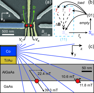
Figure 1: (a) Scanning electron micrograph showing the Ti/Au gates (yellow) used to define the DQD. Electrons tunnel sequentially from source (S) to drain (D) through the two QDs located near . The (blue) single-domain Co nanomagnet (200 (width) $\times$ 50 (height) $\times$ $2000\text{\,}{\mathrm{nm}}^{3}$, $2/5$ visible) generates an inhomogeneous magnetic field, $\mathbf{B}_{\text{nm}}$. (b) The tunneling sequence $(0\,1)\to(1\,1)\to(0\,2)\to(0\,1)$. Triplet-singlet transitions $\{T_{-},T_{0},T_{+}\}\to S_{11}$ require lifting of the PSB. (c) The relevant layers of the heterostructure, gates, and nanomagnet. The magnetic field lines (blue) are calculated according to ref. 27. The black arrows indicate the local magnetic fields $\mathbf{B}_{\text{nm}}^{\text{L}}=$032.322.4\text{\,}\mathrm{mT}$$ and $\mathbf{B}_{\text{nm}}^{\text{R}}=$05.210.6\text{\,}\mathrm{mT}$$. The $3\text{\,}\mathrm{mT}$ radius of represents the typical Overhauser field fluctuations.

We measure the current, $I$, which results from a dc voltage, here $V=1$ mV, applied across the DQD exposed to the inhomogeneous magnetic field of a nanomagnet (see Figures 1a,c). As detailed in Figure 1b, electrons tunnel sequentially through the DQD via the occupation cycle $(0\,1)\rightarrow(1\,1)\rightarrow(0\,2)\rightarrow(0\,1)$, where $(m\,n)$ indicates the number, $m$ ($n$), of electrons in the left (right) dot. The transition $(0\,1)\rightarrow(1\,1)$ loads one of four (1 1) states, which consist of the singlet state, $S_{11}$, and the three triplet states, $T_{11}=\left\{T_{-},~{}T_{0},~{}T_{+}\right\}$. Only $T_{\pm}$ have a nonzero spin projection along the quantization axis, which we choose parallel to the external magnetic field, $B_{\text{ext}}$ (along the $z$-axis in Figure 1a). The only energetically accessible (0 2) state is the singlet state, $S_{02}$. The corresponding eigenenergies are plotted in Figure 2a as a function of the energy detuning, $\Delta$, between the diabatic singlet states $S_{11}$ and $S_{02}$. The singlet eigenstates, $S_{\mathrm{s}}$ and $S_{\mathrm{a}}$, are the symmetric and antisymmetric combinations of $S_{11}$ and $S_{02}$ mixed by the interdot tunnel coupling, $t_{\text{c}}$. $T_{0}$ is at zero energy (neglecting exchange coupling), while $T_{\pm}$ are split by their Zeeman energies, $E^{\pm}_{\text{z}}=\pm g\mu_{\text{B}}\left(\left|\mathbf{B}^{\text{L}}+\mathbf{B}^{\text{R}}\right|\right)/2$, where $\mathbf{B}^{\text{L}}$ ($\mathbf{B}^{\text{R}}$) is the local magnetic field in the left (right) dot, $g$ the Landé g-factor, and $\mu_{\text{B}}$ the Bohr magneton. For $\Delta>0$, the triplets are well separated from $S_{\mathrm{s}}$, but not from $S_{\text{a}}$.

In a homogeneous magnetic field $\left(\mathbf{B}^{\text{L}}=\mathbf{B}^{\text{R}}\right)$, transitions between triplets and singlets are forbidden by Pauli spin blockade Ono et al. (2002) (PSB) (dashed arrows in Figure 1b). Eventually the occupation cycle stalls in one of the triplets resulting in $I=0$ (neglecting cotunneling). DNSP requires $I\neq 0$, which can be induced by a local field difference, $\mathbf{B}^{\text{L}}-\mathbf{B}^{\text{R}}$, that lifts the PSB by coupling triplets to singlets. One way to produce inhomogeneous fields is to include on-chip micromagnets, which have been used for all-electric control of a single electron spin Pioro-Ladriere et al. (2008); Obata et al. (2010); Brunner et al. (2011). However, at external fields below a few hundred mT, micromagnets form magnetic domains, which greatly reduce their fields. Here, we use a nanomagnet (see Figure 1a), which forms a single magnetic domain (due to its shape anisotropy) and a sizable $\Delta\mathbf{B}=\left(\mathbf{B}^{\text{L}}-\mathbf{B}^{\text{R}}\right)/2$ even if $B_{\text{ext}}=0$ Heedt et al. (2012). This previously unexplored regime proves to be highly beneficial for controlling DNSP.

Even in the absence of on-chip magnets, the HFI between thermally fluctuating nuclear spins and electrons creates an effective (Overhauser) field, $\mathbf{B}_{\text{nuc}}$, which statistically varies between the two dots resulting in a small leakage current near $B_{\text{ext}}\simeq 0$ and $\Delta\simeq 0$ Sup ; Koppens et al. (2005). Compared to $\mathbf{B}_{\text{nuc}}$, the nanomagnet’s inhomogeneous field, $\mathbf{B}_{\text{nm}}$, is more stable in time, and $\left|\Delta\mathbf{B}_{\text{nm}}\right|\gg\left|\Delta\mathbf{B}_{\text{nuc}}\right|$ (see Figure 1c). $B_{\text{ext}}$ is aligned along the easy axis (z-axis) of the nanomagnet, which has a coercive field of $52\text{\,}\mathrm{mT}$. Because the nanomagnet forms a single domain, $B_{\text{ext}}$ does not affect the magnitude of $\mathbf{B}_{\text{nm}}$. The associated $\Delta\mathbf{B}_{\text{nm}}$ results in a leakage current over a broad range of $\Delta$ and $B_{\text{ext}}$ including distinct current maxima along the $S_{\mathrm{a}}$–$T_{\pm}$ resonances (Figure 2b). These current features are seen at small $B_{\text{ext}}$ and, hence, are not accessible with multidomain magnets (see above). Our observed current features are very different from measurements performed without an on-chip magnet Sup .

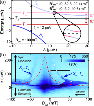
Figure 2: (a) The relevant eigenenergies as a function of $\Delta$, for $\mathbf{B}_{\text{nuc}}=0$. The inhomogeneous $\mathbf{B}_{\text{nm}}$ causes singlet-triplet mixing (see enlarged $S_{\text{a}}$–$T_{-}$ avoided crossing) and lifts the PSB. (b) Leakage current, $I$, through the DQD versus $\Delta$ (stepped from top to bottom) and $B_{\text{ext}}$ (swept at $-50$ mT$/$min). The red dashed line is a numerical prediction of the $S_{\text{a}}$–$T_{\pm}$ resonances without DNSP using $t_{\text{c}}=$12\text{\,}\mathrm{\SIUnitSymbolMicro eV}$$. The white dashed line includes DNSP (via the $S_{\mathrm{a}}$–$T_{-}$ resonance) using eq 1 with $\Gamma_{\text{rel}}=$0.043\text{\,}{\mathrm{s}}^{-1}$$, $\gamma=$10\text{\,}\mathrm{mT}$$, and $\alpha=$35\text{\,}{\mathrm{nA}}^{-1}\text{\,}{\mathrm{s}}^{-1}$$.

However, consideration of $\mathbf{B}_{\text{nm}}$ alone does not explain all features in Figure 2b. We must include the HFI and its effect on DNSP, as has proven necessary in other experiments Ono and Tarucha (2004); Vink et al. (2009); Kobayashi et al. (2011); Frolov et al. (2012). The dashed red line in Figure 2b is a prediction of the position of the $S_{\text{a}}$–$T_{\pm}$ resonances as a function of $B_{\text{ext}}$ and $\Delta$. It takes into account $\mathbf{B}_{\text{nm}}$, but neglects $\mathbf{B}_{\text{nuc}}$ Sup . Compared to this prediction, however, the measured resonances (blue arrows in Figure 2b) occur at larger $\left|B_{\text{ext}}\right|$. As we will show, this shift can be explained by including DNSP, which produces a $B_{\text{nuc}}^{z}$ that compensates $B_{\text{ext}}$, e. g., $B_{\text{nuc}}^{z}<0$ when $B_{\text{ext}}>0$.

The connection to DNSP becomes evident with the data shown in Figure 3a, which probes the $S_{\mathrm{a}}$–$T_{-}$ resonance as a function of time for a fixed $\Delta$. We prepared the nuclear spin polarization, $P$, to $P\simeq 0$ by waiting three minutes at $I=0$ before turning on the voltage across the DQD. The current maximum, $I_{\text{max}}$, at the $S_{\mathrm{a}}$–$T_{-}$ resonance occurs later in time at larger $B_{\text{ext}}$. Again, this can be explained if $B^{z}_{\text{nuc}}<0$ and compensates $B_{\text{ext}}$. Because the GaAs g-factor is negative, $P=-B_{\text{nuc}}^{z}/B^{\text{max}}_{\text{nuc}}$, where $B^{\text{max}}_{\text{nuc}}\simeq 6.1$ T is the Overhauser field magnitude produced when all nuclear spins are aligned Sup . $B^{z}_{\text{nuc}}<0$ implies that $P>0$, which can only be explained if DNSP from $T_{+}$ outweighs that from $T_{-}$, despite the system being near the $S_{\text{a}}$–$T_{-}$ resonance. This peculiar situation results from spin-selective lifting of the PSB (of $T_{-}$) and bolsters DNSP, as discussed below.

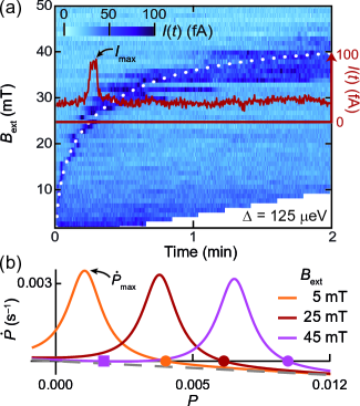
Figure 3: (a) Current versus time, $I(t)$, as a function of $B_{\text{ext}}$ along the horizontal line in Figure 2b (we prepared $P(0)=0$). Density Plot: $I(t,B_{\text{ext}})$. The white dotted line predicts the moment of maximal current, $t\left(I_{\text{max}}\right)$, using eq 1 and the same parameters as in Figure 2b. Red Trace: $I(t)$ measured at $B_{\text{ext}}=$25\text{\,}\mathrm{mT}$$. (b) $\dot{P}(P)$ for three different $B_{\text{ext}}$ using eq 1 and the same parameters as in Figure 2b. Far from resonance an exponential decay $\dot{P}=-\Gamma_{\text{rel}}P$ remains (gray dashed line). $\CIRCLE$,$\CIRCLE$,$\CIRCLE$ mark the $B_{\text{ext}}$–dependent “adjustable” fixed point and $\blacksquare$ a “trivial” fixed point, which appears near $P=0$ when $B_{\text{ext}}\gtrsim$45\text{\,}\mathrm{mT}$$.

Our explanation starts with a rate equation model Vink et al. (2009); Danon et al. (2009); Rudner et al. (2011a) including only polarization generated by $T_{+}$ near the $S_{\text{a}}$–$T_{-}$ resonance (A comprehensive calculation in Sup Sec. III includes all (1 1) states). As a simplification, we use the average polarization $P=\left(P^{\text{L}}+P^{\text{R}}\right)/2$. ($P^{\text{L}}\neq P^{\text{R}}$ would mainly affect the decay of $T_{0}$, not $T_{\pm}$.) The overall rate equation is

$$\dot{P}(t)=\Gamma_{\text{pol}}(t)\left[1-P(t)\right]-\Gamma_{\text{rel}}P(t),$$ (1)

where the polarization decay rate, $\Gamma_{\text{rel}}$, is constant, while the build-up rate, $\Gamma_{\text{pol}}(t)$, is proportional to current, $\Gamma_{\text{pol}}(t)=\alpha I(t)>0$, as observed experimentally. For convenience, we describe the current maximum at the $S_{\mathrm{a}}$–$T_{-}$ resonance as a Lorentzian

$$I(t)=I_{\text{max}}\frac{\left(\gamma/2\right)^{2}}{\left(E^{-}_{z}-E_{\text{a}}\right)^{2}+\left(\gamma/2\right)^{2}},$$ (2)

where $I_{\text{max}}$ is the (measured) resonant current and $\gamma$ is the effective width of the resonance. (Nonresonant states contribute weakly to $I(t)$.) Here

$$E_{\text{a}}=\left(-\Delta+\sqrt{t_{\text{c}}^{2}+\Delta^{2}}\right)/2$$ (3)

is the energy of $S_{\text{a}}$. We approximate $E_{\text{z}}$ by only including the average $z$-component of $\mathbf{B}_{\text{nm}}$, $\overline{B}^{z}_{\text{nm}}$, so that

$$E^{-}_{\text{z}}\approx\left|g\right|\mu_{\text{B}}\left(B_{\text{ext}}(t)-B^{\text{max}}_{\text{nuc}}P(t)+\overline{B}^{z}_{\text{nm}}\right).$$ (4)

Example $\dot{P}(P)$ curves are plotted in Figure 3b and are used to model the data in Figure 3a. $P\left(t=0\right)=0$ in this measurement, and the model predicts $\dot{P}(P=0)>0$ (evident in Figure 3b). Therefore, $P$ increases in time until it reaches a stable fixed point at $\dot{P}=0$ (and $\text{d}\dot{P}/\text{d}P<0$). For $B_{\text{ext}}<$43\text{\,}\mathrm{mT}$$, $P$ passes through the $S_{\mathrm{a}}$–$T_{-}$ resonance, which coincides with $\dot{P}_{\text{max}}$ in Figure 3b. As $B_{\text{ext}}$ is increased, the $S_{\mathrm{a}}$–$T_{-}$ resonance moves to larger $P$, and with it move $\dot{P}_{\text{max}}$ and the stable “adjustable” fixed point (A-FP, circles in Figure 3b). Accordingly, the measured (resonant) $I_{\text{max}}$ in Figures 3a appears later in time with increasing $B_{\text{ext}}$. When $B_{\text{ext}}\approx$45\text{\,}\mathrm{mT}$$, a second stable “trivial” fixed point (T-FP, square in Figure 3b) appears near $P=0$ and remains there for $B_{\text{ext}}>$45\text{\,}\mathrm{mT}$$. Hence, we expect $P$ to remain near zero (far from resonance) at the T-FP. Indeed, no resonant current maximum is observed for $B_{\text{ext}}\gtrsim$43\text{\,}\mathrm{mT}$$ in Figure 3a.

Eq 1 provides quantitative predictions of the time evolution of the $S_{\mathrm{a}}$–$T_{-}$ resonance associated with the measured $I_{\text{max}}$. Namely, it yields the white fits in Figures 2b and 3a. These two separate fits share altogether four fit parameters. The agreement between our model and data indicates that the model captures the DNSP in both experiments. In addition, $\Gamma_{\text{rel}}$ agrees with reported values Reilly et al. (2010).

Our model reveals a straightforward procedure to maximize $P$. We start at small $B_{\text{ext}}$ where the T-FP is absent and $P$ is initialized at the A-FP (see top panel of Figure 4a). This initialization requires small $B_{\text{ext}}$ and sufficient singlet–triplet mixing and is only possible with a single-domain nanomagnet. To reach a large $P$, we increase $B_{\text{ext}}$ (with a sufficiently slow sweep rate) dragging the A-FP, and $P$ along with it (see middle panel of Figure 4a). This dragging procedure works up to a maximum polarization, $P_{\text{max}}$, occurring when the decay of $P$ overwhelms its build-up and $\dot{P}_{\text{max}}=0$ (see bottom panel of Figure 4a). $P_{\text{max}}$ is defined by solving eq 1 for $\dot{P}(P_{\text{max}})=0$:

$$P_{\text{max}}/\left(1-P_{\text{max}}\right)=\alpha I_{\text{max}}/\Gamma_{\text{rel}}\equiv\Gamma_{\text{pol}}^{\text{max}}/\Gamma_{\text{rel}},$$ (5)

where $\Gamma_{\text{pol}}^{\text{max}},P_{\text{max}}>0$ and both depend on $\Delta$ via $I_{\text{max}}$. At $B^{\text{max}}_{\text{ext}}$ (the field corresponding to $P_{\text{max}}$), the A-FP coincides with the $S_{\text{a}}$–$T_{-}$ resonance, and we expect a current maximum.

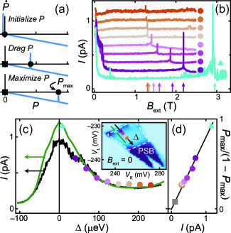
Figure 4: (a) $\dot{P}(P)$ for three $B_{\text{ext}}$ using eq 1 with $I_{\text{max}}=$1.2\text{\,}\mathrm{pA}$$ and the fit parameters from Figure 2b. $\blacksquare$ marks the T-FP and $\CIRCLE$ the A-FP. (b) Leakage current, $I$, for various $\Delta$ in the PSB regime [see (c)] measured while continuously increasing $B_{\text{ext}}$ (at 30 mT$/$min) after initialization at the A-FP at $B_{\text{ext}}=$50\text{\,}\mathrm{mT}$$. (All but the lowest trace are vertically offset in increments of 125 fA.) Sharp current peaks (marked by arrows) correspond to the maximum polarization, $P_{\text{max}}(\Delta)$, in (a). (c) $P_{\text{max}}/\left(1-P_{\text{max}}\right)$ from (b) (filled circles) and $I$ (black/green traces), measured along the (black/green) lines in the inset, versus $\Delta$. Inset: $I$ measured as a function of gate voltages $V_{\text{L,R}}$ (see Figure 1a). The region of suppressed $I$ within the double triangle of finite current marks PSB. (d) $P_{\text{max}}/\left(1-P_{\text{max}}\right)$ versus $I$, extracted from the traces in (c). The gray square is predicted from the data in Figure 2b. The black line expresses eq 5 with $\alpha/\Gamma_{\text{rel}}=$0.81\text{\,}{\mathrm{pA}}^{-1}$$ using the fit parameters from Figure 2b.

Indeed, the leakage current measured during such DNSP sweeps, displayed for various $\Delta$ in Figure 4b, features a sharp current maximum at a particular $B_{\text{ext}}$ (see arrows), which we identify as $B^{\text{max}}_{\text{ext}}(\Delta)$. For $B_{\text{ext}}>B^{\text{max}}_{\text{ext}}$, the A-FP is lost, and the nuclear spin polarization decays ($\dot{P}<0$) with rate $\Gamma_{\text{rel}}$.

$P_{\text{max}}(\Delta)$ compensates $B^{\text{max}}_{\text{ext}}(\Delta)$ so that we can equate $P_{\text{max}}(\Delta)=B^{\text{max}}_{\text{ext}}(\Delta)/B^{\text{max}}_{\text{nuc}}$ . $P_{\text{max}}/(1-P_{\text{max}})$ and $I$ measured versus $\Delta$ are shown side-by-side in Figure 4c demonstrating a striking correlation between $P_{\text{max}}/(1-P_{\text{max}})$ and $I$. In fact, in accordance with eq 5, Figure 4d shows that $P_{\text{max}}/\left(1-P_{\text{max}}\right)\propto I$ confirming our assumption that $\Gamma_{\text{pol}}\propto I$. The straight black line in Figure 4d expresses eq 5 using the fit parameters from Figure 2b. The ability to explain three very different data sets (Figures 2b, 3a, 4d) with one set of fit parameters corroborates the interpretation of the current peaks in Figure 4b and the validity of our rate equation model Sup .

Our highest $B^{\text{max}}_{\text{ext}}\simeq$2.9\text{\,}\mathrm{T}$$ (green data in Figure 4b) corresponds to $P\simeq$50\text{\,}\mathrm{\char 37\relax}$$ (and generates an Overhauser field gradient of $\sim$1\text{\,}\mathrm{T}\mathrm{/}{100\mathrm{n}\mathrm{m}}$$ across the DQD boundary). This exceeds by far previously reported polarizations in laterally defined DQDs Laird et al. (2007); Petta et al. (2008); Foletti et al. (2009); Reilly et al. (2010)(a complementary measurement of P in Sup Sec. VI).

To detail how $\mathbf{B}_{\text{nm}}$ and the HFI combine to lift the PSB and induce DNSP, we compare our system with two simpler scenarios. If the HFI were the only mechanism to lift PSB, no DNSP would be expected since all triplets are loaded equally often resulting in as many up as down nuclear spin flips. In experiments without a nanomagnet Baugh et al. (2007); Kobayashi et al. (2011), cotunneling weakly lifts the PSB (in competition with the HFI) and does so equally for each triplet, nearly irrespective of its energy. In contrast, the hyperfine-induced decay rate is strongly energy dependent. Therefore, near the $S_{\text{a}}$–$T_{-}$ resonance, $T_{-}$ generates more nuclear spin flips than $T_{+}$, and $P<0$ is observed without nanomagnet.

In our case, $\mathbf{B}_{\text{nm}}$ mixes $T_{-}$ and $S_{\mathrm{a}}$ strongly near their resonance, resulting in two (1 1) states that are no longer in PSB. Hyperfine-induced decay is heavily suppressed in these mixed states. In this situation, the HFI still contributes to the decay of $T_{+}$ (and $T_{0}$) thereby producing DNSP and $P>0$. In an alternative approach, DNSP has been studied for large $t_{\text{c}}$ ($\sim$100\text{\,}\mathrm{\SIUnitSymbolMicro eV}$$) by sweeping $\Delta$Baugh et al. (2007); Kobayashi et al. (2011); Frolov et al. (2012). However, when $t_{\text{c}}\sim$110\text{\,}\mathrm{\SIUnitSymbolMicro eV}$$, which is favorable for spin qubits, $P$ is limited by the energy of $S_{\text{a}}$ in the PSB regime, so that $\left|P\right|\lesssim t_{\text{c}}/\left(2\left|g\right|\mu_{\text{B}}B^{\text{max}}_{\text{nuc}}\right)\sim$10\text{\,}\mathrm{\char 37\relax}$$. Moreover, $B_{\text{nuc}}^{z}<0$ in our system provides a distinct advantage because $B_{\text{nuc}}^{z}$ compensates $B_{\text{ext}}$ such that the total effective magnetic field is constant during the polarization build-up; therefore, $P$ is only limited by $\alpha I_{\text{max}}/\Gamma_{\text{rel}}$ when dragging $P$ with $B_{\text{ext}}$.

We have demonstrated a nuclear spin polarization of $\simeq$50\text{\,}\mathrm{\char 37\relax}$$ in a DQD based on the enhanced ability to manipulate the nuclear spin ensemble using an on-chip nanomagnet. Larger polarizations can be expected upon further optimization of the electronic spectrum, sample geometry and materials. Our results demonstrate the flexibility offered by an on-chip nanomagnet, which could be used for all-electric ESR Pioro-Ladriere et al. (2008) while simultaneously polarizing the nuclear spin ensemble at small $t_{\text{c}}$ values ideal for spin qubit operation. Such a system could be used to improve nuclear state preparation techniques Giedke et al. (2006); Reilly et al. (2008); Foletti et al. (2009); Issler et al. (2010) or for measuring complex nuclear phenomena such as spin squeezing Rudner et al. (2011b), quantum memory Taylor et al. (2003); Kurucz et al. (2009), dark states Gullans et al. (2010), quantum phase transitions Rudner and Levitov (2010), and superradiance Schuetz et al. (2012).

I Supplementary Information for “Large nuclear spin polarization in gate-defined quantum dots using a single-domain nanomagnet”

Contents

1. I Supplementary Information for “Large nuclear spin polarization in gate-defined quantum dots using a single-domain nanomagnet”
2. II I. Overview
3. III II. Sample Design and Experimental Setup
4. IV III. The Hamiltonian
   1. V IV. Perturbation calculation of DNSP
   2. VI V. Hyperfine- and Non-hyperfine–induced Leakage Current
   3. VII VI. Nuclear Polarization Build-up
   4. VIII VII. Data Fitting

II I. Overview

The following supplementary material provides additional information related to various aspects of the main article. We start in Section IIIII with details about the sample design and the experimental setup of the measurements. In Section IIIIV we introduce a model Hamilton operator which describes the hyperfine interaction (HFI) in our double quantum dot (DQD) setup including the inhomogeneous magnetic field of the nanomagnet. Based on a rate equation model, in Section IVV, we perturbatively solve the dynamic nuclear spin polarization (DNSP) problem by explicitly taking into account the contributions of all four (1 1) states. We show that the perturbative solution justifies the simplified model used in the main article. Section VVI provides detailed explanations of the current features in Fig. 2b of the main article. In Section VIVII we present results of a complementary experiment that gives additional evidence of the validity of our model and of our interpretation of the data in Fig. 4 of the main article in terms of a large nuclear spin polarization. Section VIIVIII describes the fitting procedure for the data in Figs. 2b, 3a of the main article.

III II. Sample Design and Experimental Setup

The samples have been fabricated from a GaAs / AlGaAs heterostructure containing a two-dimensional electron system (2DES) $85\text{\,}\mathrm{nm}$ below the surface. At cryogenic temperatures, the 2DES has a carrier density of $1.19\text{\times}{10}^{11}\text{\,}{\mathrm{cm}}^{-2}$ and a mobility of $0.36\text{\times}{10}^{6}\text{\,}{\mathrm{cm}}^{2}\text{\,}{\mathrm{V}}^{-1}\text{\,}{\mathrm{s}}^{-1}$. Metallic gate electrodes (30 nm gold on top of 5 nm titanium) have been fabricated on the sample surface by electron-beam lithography and standard evaporation/lift-off techniques (Fig.  S1a). The Co nanomagnet with a thickness of $50\text{\,}\mathrm{nm}$ was evaporated directly on top of the leftmost gate and capped with $5\text{\,}\mathrm{nm}$ of Au to prevent oxidization. Negative voltages applied to these electrodes are used to deplete locally the 2DES and thereby define the DQD. The absolute electron occupation, ($m~{}n$), was determined by quantum-point-contact charge detectionJohnson et al. (2005). All measurements have been performed in a dilution refrigerator at an electron temperature of $\sim$100\text{\,}\mathrm{mK}$$. Fig. S1b sketches the experimental situation in this Letter. A source-drain voltage of $V=(\mu_{\text{S}}-\mu_{\text{D}})/e$ is applied across the DQD between degenerate leads. The DQD is in the Pauli-spin blockade, where a triplet state can only contribute to current if it is coupled to a singlet state, e.g., by field inhomogeneity or interaction with the ensemble of $N_{\text{L(R)}}\sim 10^{6}$ nuclei.

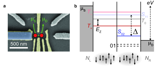
Figure S1: Experimental setup a) SEM image of the DQD device used in the experiments. b) A DQD in Pauli-spin blockade (typical experimental situation), while a voltage $V$ is applied between the degenerate 2D leads with chemical potentials $\mu_{\text{S}}$ and $\mu_{\text{D}}$. Vertical lines are tunnel barriers. The right dot always contains at least one electron. The dashed horizontal lines are the spin-split chemical potentials of the spin up/down (0 1) states, where the chemical potential of a quantum dot is defined as the energy needed to add one more electron. The solid horizontal lines are the chemical potentials of the five relevant two-electron basis states, where $E_{\text{Z}}$ is the Zeeman energy and $\Delta$ is the energy detuning between the singlet states, $S_{11}$ and $S_{02}$.

IV III. The Hamiltonian

The total Hamiltonian of the system includes electrostatic, magnetic, and hyperfine contributions and is given (in the relevant subspace depicted in Fig. S1b) by

$$H=H_{\text{el}}+H_{\text{B}}+H_{\text{hf}}.$$ (S1)

Using the diabatic singlet-triplet basis $\left\{T_{+},T_{0},T_{-},S_{11},S_{02}\right\}$, the electrostatic contribution is

$$H_{\text{el}}=t_{\text{c}}/2\left(\left|S_{11}\vphantom{S_{02}}\right\rangle\left\langle S_{02}\vphantom{S_{11}}\right|+\left|S_{02}\vphantom{S_{11}}\right\rangle\left\langle S_{11}\vphantom{S_{02}}\right|\right)-\Delta\left|S_{02}\vphantom{S_{02}}\right\rangle\left\langle S_{02}\vphantom{S_{02}}\right|,$$ (S2)

where $\Delta$ is the interdot energy detuning (see Fig. S1) and $t_{\text{c}}$ is the interdot tunnel splitting (see Fig. 2a of the main article). The interaction between the local magnetic fields and the electron spins in the two dots is described by

$$H_{\text{B}}=g\mu_{\text{B}}\left[\left(\mathbf{B}_{\text{ext}}+\mathbf{B}_{\text{nm}}^{\text{L}}\right)\cdot\mathbf{S}^{\text{L}}+\left(\mathbf{B}_{\text{ext}}+\mathbf{B}_{\text{nm}}^{\text{R}}\right)\cdot\mathbf{S}^{\text{R}}\right],$$ (S3)

where $\mathbf{B}_{\text{ext}}$ is the external magnetic field, $\mathbf{B}_{\text{nm}}^{\text{L,R}}$ the local magnetic field of the nanomagnet, $\mathbf{S}^{\text{L,R}}$ the local electron spin operator, $g$ the electron g-factor, and $\mu_{\text{B}}$ the Bohr magneton.

The wave function of an electron confined in a lateral GaAs-dot overlaps with $\sim 10^{6}$ nuclei. The hyperfine interaction between the electron spin and the nuclear spins is dominated by the contact term $H^{\text{L,R}}_{\text{con}}=\sum_{k}A^{\text{L,R}}_{k}\mathbf{I}^{\text{L,R}}_{k}\cdot\mathbf{S}^{\text{L,R}}$, where $\mathbf{I}^{\text{L,R}}_{k}$ is the $k$th nuclear spin operator and $A^{\text{L,R}}_{k}$ the hyperfine coupling constants. $A^{\text{L,R}}_{k}$ is proportional to the overlap between the wavefunctions of the $k$th nucleus in left/right dot and the electron and varies by isotope type. It is common to define an average $A$ reflecting the natural abundance of isotope type and the average overlap with the electron wavefunction. In this approximation, the contact Hamiltonian is $H^{\text{L,R}}_{\text{con}}=A\mathbf{I}^{\text{L,R}}\cdot\mathbf{S}^{\text{L,R}}$, where $\mathbf{I}^{\text{L,R}}$ is the average nuclear spin (ensemble) operator and $A=$85\text{\,}\mathrm{\SIUnitSymbolMicro eV}$$ in GaAsCoish and Baugh (2009). Electrons in the left/right dot couple to different sets of nuclei, and we can write

$$H_{\text{hf}}=H^{\text{L}}_{\text{con}}+H^{\text{R}}_{\text{con}}=A\left(\mathbf{I}^{\text{L}}\cdot\mathbf{S}^{\text{L}}+\mathbf{I}^{\text{R}}\cdot\mathbf{S}^{\text{R}}\right)=A\sum_{i=\text{L,R}}\left(I_{z}^{i}S_{z}^{i}+\frac{I_{+}^{i}S_{-}^{i}+I_{-}^{i}S_{+}^{i}}{2}\right),$$ (S4)

where $S^{\text{L,R}}_{z}$ and $I^{\text{L,R}}_{z}$ are the corresponding $z$-projection operators; and $S^{\text{L,R}}_{\pm}=S^{\text{L,R}}_{x}\pm iS^{\text{L,R}}_{y}$ and $I^{\text{L,R}}_{\pm}=I^{\text{L,R}}_{x}\pm iI^{\text{L,R}}_{y}$ are the spin raising and lowering operators. In a semiclassical approximation $\mathbf{I}^{\text{L,R}}$ can be replaced by the effective nuclear magnetic (Overhauser) fieldOverhauser (1953) $\mathbf{B}_{\text{nuc}}^{\text{L,R}}=A\left<\mathbf{I}^{\text{L,R}}\right>/\left(g\mu_{\text{B}}\right)$, where $\left<\ldots\right>$ denotes the expectation value, and $\left<I\right>_{\text{max}}=3/2$ in GaAs. In ESR experiments (not shown), we measured $g\simeq-0.36$ in our system. This predicts, for fully polarized nuclear spins ($P=1$), an Overhauser field magnitude of $B^{\text{max}}_{\text{nuc}}=A\left<I\right>_{\text{max}}/\left(\left|g\right|\mu_{\text{B}}\right)\simeq$6.1\text{\,}\mathrm{T}$$. The semiclassical version of $H_{\text{hf}}$ has the same form as $H_{\text{B}}$ (see Eq. (S3)), and we can summarize

$$H_{\text{B}}+H_{\text{hf}}=g\mu_{\text{B}}\left(\mathbf{B}^{\text{L}}\cdot\mathbf{S}^{\text{L}}+\mathbf{B}^{\text{R}}\cdot\mathbf{S}^{\text{R}}\right),$$ (S5)

where $\mathbf{B}^{\text{L,R}}=\mathbf{B}_{\text{ext}}+\mathbf{B}_{\text{nm}}^{\text{L,R}}+\mathbf{B}_{\text{nuc}}^{\text{L,R}}$ is the total effective magnetic field acting on an electron in the left and right dot, respectively.

In analogy to $\overline{\mathbf{B}}=\left(\mathbf{B}^{\text{L}}+\mathbf{B}^{\text{R}}\right)/2$ and $\Delta\mathbf{B}=\left(\mathbf{B}^{\text{L}}-\mathbf{B}^{\text{R}}\right)/2$, we define the symmetric and antisymmetric spin operators $\overline{\mathrm{S}}=\left(\mathbf{S}^{\text{L}}+\mathbf{S}^{\text{R}}\right)/2$ and $\Delta\mathrm{S}=\left(\mathbf{S}^{\text{L}}-\mathbf{S}^{\text{R}}\right)/2$. We then use $\overline{B}_{\pm}=\overline{B}_{x}\pm i\overline{B}_{y}$, $\Delta B_{\pm}=\Delta B_{x}\pm i\Delta B_{y}$, $\overline{\mathrm{S}}_{\pm}=\overline{\mathrm{S}}_{x}\pm i\overline{\mathrm{S}}_{y}$ and $\Delta\mathrm{S}_{\pm}=\Delta\mathrm{S}_{x}\pm i\Delta\mathrm{S}_{y}$, defined akin to the spin raising and lowering operators in equation (S4), to write equation (S5) analogous to the right hand side of equation (S4):

$$H_{\text{B}}+H_{\text{hf}}=g\mu_{\text{B}}\left(2\overline{B}_{z}\overline{\mathrm{S}}_{z}+2\Delta B_{z}\Delta\mathrm{S}_{z}+\Delta B_{+}\Delta\mathrm{S}_{-}+\Delta B_{-}\Delta\mathrm{S}_{+}+\overline{B}_{+}\overline{S}_{-}+\overline{B}_{-}\overline{S}_{+}\right).$$ (S6)

With the quantization axis, $\hat{z}$, defined parallel to $\mathbf{B}_{\text{ext}}$, the matrix representation of the (semiclassical) total Hamiltonian in the basis spanned by the diabatic singlet and triplet states {$T_{+}$, $T_{0}$, $T_{-}$, $S_{11}$, $S_{02}$} is

$\displaystyle H=\mu^{\star}\;$ ccccc@      —@  c        $T_{+}$        &        $T_{0}$               $T_{-}$               $S_{11}$               $S_{02}$

(ccccc)@      —@  l $\displaystyle\sqrt{2}\ \overline{B}_{z}$ $\overline{B}_{-}$ $0$ $-\Delta B_{-}$ $0$ $T_{+}=\left|\uparrow\uparrow\right\rangle$

$\overline{B}_{+}$ $0$ $\overline{B}_{-}$ $\sqrt{2}\Delta B_{z}$ $0$ $T_{0}=\left(\left|\uparrow\downarrow\right\rangle+\left|\downarrow\uparrow\right\rangle\right)/\sqrt{2}$

$0$ $\overline{B}_{+}$ $-\sqrt{2}\ \overline{B}_{z}$ $\Delta B_{+}$ $0$ $T_{-}=\left|\downarrow\downarrow\right\rangle$

$-\Delta B_{+}$ $\sqrt{2}\Delta B_{z}$ $\Delta B_{-}$ $0$ $t_{\text{c}}^{\star}/2$ $S_{11}=\left(\left|\uparrow\downarrow\right\rangle-\left|\downarrow\uparrow\right\rangle\right)/\sqrt{2}$

$0$ $0$ $0$ $t_{\text{c}}^{\star}/2$ $-\Delta^{\star}$ $S_{02}=\left|0,\uparrow\downarrow\right\rangle$

(S7)

where $\mu^{\star}=g\mu_{\text{B}}/\sqrt{2}$, $t_{\text{c}}^{\star}=t_{\text{c}}/\mu^{\star}$ and $\Delta^{\star}=\Delta/\mu^{\star}$. The matrix representation (S7) illustrates that the $x$- and $y$-components of $\Delta\mathbf{B}$ mix $T_{\pm}$ with $S_{11}$, while the $z$-component of $\Delta\mathbf{B}$ mixes $T_{0}$ (which has no spin component along the $z$-axis) with $S_{11}$. Instead, $\overline{B}_{z}$ leads to the Zeeman splitting of the $T_{\pm}$ states. Note that the off-diagonal terms $\overline{B}_{\pm}$, which mix $T_{\pm}$ with $T_{0}$, vanish if the quantization axis is chosen parallel to $\overline{\mathbf{B}}$.

V IV. Perturbation calculation of DNSP

In the main article, we use a simplified approximation that only considers the hyperfine contribution from $T_{+}$. In this section, we calculate the hyperfine-induced decay of all (1 1) states using perturbation theory (Fermi’s golden rule) similar to reference Rudner et al. (2011) in which, however, the effects of a nanomagnet were not included. Here we show that the simplified model produces the pertinent features of the perturbation theory, justifying the approximation used in the main article.

We start by writing equation (S1) as $H=H_{0}+H^{+}_{\text{ff}}+H^{-}_{\text{ff}}$, where

$$H_{0} =H_{\text{el}}+H_{\text{B}}+2g\mu_{\text{B}}\left(\overline{B}^{z}_{\text{nuc}}\overline{S}_{z}+\Delta B^{z}_{\text{nuc}}\Delta S_{z}\right)\,,$$ (S8)

$$H^{\pm}_{\text{ff}} =g\mu_{\text{B}}\left(\overline{B}_{\text{nuc}}^{\pm}\overline{\mathrm{S}}_{\mp}+\Delta B_{\text{nuc}}^{\pm}\Delta\mathrm{S}_{\mp}\right)\,,$$ (S9)

are the bare Hamiltonian and hyperfine flip-flop Hamiltonians, respectively. We treat $H^{+}_{\text{ff}}+H^{-}_{\text{ff}}$ as a perturbation of $H_{0}$. Diagonalization of $H_{0}$ provides the unperturbed eigenvalues, $E_{n}$, of the $n$th eigenstate, $\left|n\right\rangle$. We account for coupling to the leads by a simple master equation with four Lindblad operators (eliminating the intermediate stage in the sequential tunneling process $(0\,2)\to(0\,1)\to(1\,1)$) and assuming that the four (1 1) states $\{T_{+},T_{0},T_{-},S_{11}\}$ are populated with equal rate:

$$\frac{d}{dt}\rho=\frac{1}{i\hbar}[H_{0},\rho]+\frac{\Gamma_{R}}{4}\sum_{x\in\{T_{+},T_{0},T_{-},S_{11}\}}\left(\left|x\vphantom{S_{02}}\right\rangle\left\langle S_{02}\vphantom{x}\right|\rho\left|S_{02}\vphantom{x}\right\rangle\left\langle x\vphantom{S_{02}}\right|-\frac{1}{2}\left(\left|S_{02}\vphantom{S_{02}}\right\rangle\left\langle S_{02}\vphantom{S_{02}}\right|\rho+\rho\left|S_{02}\vphantom{S_{02}}\right\rangle\left\langle S_{02}\vphantom{S_{02}}\right|\right)^{\phantom{X}}\!\!\!\!\right).$$ (S10)

We approximate the dynamics by a rate equation for the populations $\boldsymbol{\rho}=(\rho_{11},\rho_{22},\rho_{33},\rho_{44},\rho_{55})$ in the five energy eigenstates.

$$\frac{d\boldsymbol{\rho}}{dt}=G^{(0)}\boldsymbol{\rho}.$$ (S11)

The transition matrix $G^{(0)}=(G^{(0)}_{ij})_{ij}$, describes decay of the level $n$ with a rate $\Gamma_{n}^{0}=\Gamma_{R}s_{n}$, determined by $s_{n}=|\left\langle S_{02}\vphantom{n}\right|\left.n\vphantom{S_{02}}\right\rangle|^{2}$, the overlap of $\left|n\right\rangle$ with the localized singlet state. Since only (1 1) states are refilled, the rate with which $\left|m\right\rangle$ is populated is proportional to $(1-s_{m})$: Hence the matrix elements of $G^{(0)}$ are

$$G^{(0)}_{nm} =\phantom{-}\frac{\Gamma_{R}}{4}(1-s_{n})s_{m}\,\,\,(n\not=m),$$ (S12)

$$G^{(0)}_{nn} =-\frac{\Gamma_{R}}{4}s_{n}\left(3+s_{n}\right).$$ (S13)

The width of the level $\left|n\right\rangle$ is given by $\hbar\Gamma^{0}_{n}=\hbar\Gamma_{R}s_{n}$.

We include the hyperfine flip-flop processes using Fermi’s golden rule (assuming a constant density of states over the range of energies of the (1 1) states) to determine the flip-flop rate from an initial state, $\left|n\right\rangle$, to the final state, $\left|f\right\rangle$ as

$$\Gamma^{\pm}_{n\to f} =\dfrac{2\pi}{\hbar}\left|\left<f\vphantom{H^{\pm}_{\text{ff}}n}\right|H^{\pm}_{\text{ff}}\left|n\vphantom{fH^{\pm}_{\text{ff}}}\right>\right|^{2}\dfrac{1}{2\pi}\dfrac{\hbar\left(\Gamma^{0}_{f}+\Gamma^{0}_{n}\right)}{\left(E_{n}-E_{f}\right)^{2}+\left(\hbar\frac{\Gamma^{0}_{f}+\Gamma^{0}_{n}}{2}\right)^{2}}\frac{1\mp P}{2}$$

$$=\dfrac{\left|\left<f\vphantom{H^{\pm}_{\text{ff}}n}\right|H^{\pm}_{\text{ff}}\left|n\vphantom{fH^{\pm}_{\text{ff}}}\right>\right|^{2}\left(\Gamma^{0}_{f}+\Gamma^{0}_{n}\right)}{\left(E_{n}-E_{f}\right)^{2}+\left(\hbar\frac{\Gamma^{0}_{f}+\Gamma^{0}_{n}}{2}\right)^{2}}\frac{1\mp P}{2},$$

where the factor $\left(1\mp P\right)/2$ expresses the influence of polarization on the nuclear-spin flip rates. The total escape rate from $\left|n\right\rangle$ is then

$$\Gamma_{n}=\Gamma^{0}_{n}+\sum_{f\not=n}(\Gamma^{+}_{n\to f}+\Gamma^{-}_{n\to f}).$$ (S14)

We can neglect cotunneling in our sample, since its contribution to the leakage current is negligible compared to that of the nanomagnet. The full rate equation is now given by

$$\frac{d\boldsymbol{\rho}}{dt}=G\boldsymbol{\rho},$$ (S15)

with $G_{nm}=G^{(0)}_{nm}+\Gamma^{+}_{n\to m}+\Gamma^{-}_{n\to m}(n\not=m)$ and $G_{nn}=G^{(0)}_{nn}-\sum_{m\not=n}(\Gamma^{+}_{n\to m}+\Gamma^{-}_{n\to m})$.

We determine the leakage current and the DNSP rates by numerically solving for $\dot{\boldsymbol{\rho}}=0$, obtaining the steady state populations $\rho^{\text{ss}}_{n}$. The magnitude of the total current is given by

$$I=I^{0}+I^{+}+I^{-}=e\sum_{n}{\rho^{\text{ss}}_{n}\Gamma_{n}},$$

where $e$ is the magnitude of the electron charge. $I^{0}$ is the non-polarizing current induced by the nanomagnet, while $I^{\pm}$ are the hyperfine-generated currents that polarize in opposite directions. $I^{\pm}$ are expressed as

$$I^{\pm}=e\sum_{n}{\rho_{n}\Gamma^{\pm}_{n}}.$$

To convert these currents into nuclear polarization rates, we write

$$\Gamma^{\pm}_{\text{pol}}=\frac{2I^{\pm}}{eN},$$

where we have normalized by $e$ and included that the polarization, $P=\left(N^{\uparrow}-N^{\downarrow}\right)/N$, changes by $2/N$ per nuclear spin flip for $N$ nuclei in total. The overall polarization rate equation is

$$\dot{P}=\Gamma^{+}_{\text{pol}}-\Gamma^{-}_{\text{pol}}-P\Gamma_{\text{rel}}.$$ (S16)

In the main article, we neglect $\Gamma^{-}_{\text{pol}}$ and approximate

$$\dot{P}\simeq\Gamma^{+}_{\text{pol}}-P\Gamma_{\text{rel}}\simeq\alpha I\left(1-P\right)-P\Gamma_{\text{rel}},$$ (S17)

where $\alpha$ is taken as a constant ($\sim$35\text{\,}{\mathrm{nA}}^{-1}\text{\,}{\mathrm{s}}^{-1}$$).

To compare the above theoretical model with the simplified version used in the main text, Fig. S2 shows $\dot{P}$ versus $P$ and $B_{\text{ext}}$ predicted using the two models represented by equations (S16) and (S17). The simple model, shown in Fig. S2a, predicts a narrow region of positive $\dot{P}$ running diagonally through the $P$–$B_{\text{ext}}$ plane. The perturbation theory calculation, shown in Fig. S2b, predicts this same feature, which is associated with the $S_{\text{a}}$–$T_{-}$ resonance, as well as more complicated behavior associated with other singlet–triplet resonances (see Fig. S2c). Both models predict that the $S_{\text{a}}$–$T_{-}$ resonance is the only resonance which creates a stable fixed point at large $P$ and $B_{\text{ext}}$. Figs. S2c-e demonstrate the good agreement between the simplified model (orange lines) and the perturbation calculation (black lines) at the $S_{\text{a}}$–$T_{-}$ resonance. (The orange lines here are the same as the lines in Fig. 4a of the main article.) Compared to the other two resonances, $\dot{P}$ at the $S_{\text{a}}$–$T_{\pm}$ resonances is very steep and provides strong feedback of the nuclear spins toward the A-FP, a distinct advantage for DNSP. From Fig. S2, it is evident that equations (1–4) of the main article are sufficient to model the nuclear polarization associated with the $S_{\text{a}}$–$T_{-}$ resonance.

The leftmost and rightmost $\dot{P}$ extrema in Figs. S2c-d are generated by the $S_{\mathrm{s}}$–$T_{\pm}$ resonances, while the small feature between the $S_{\text{a}}$–$T_{\pm}$ resonances corresponds to the crossing of the triplet levels at $B^{z}=B_{\text{ext}}+\overline{B}^{z}_{\text{nm}}-PB_{\text{nuc}}^{\text{max}}\approx 0$. Note that the nuclear field components $\bar{B}_{\text{nuc}}^{x,y},\Delta B^{x,y,z}_{\text{nuc}}$ play an important role for our treatment, determining directly the strength of the hyperfine flip-flop rates. For the DNSP rates depicted in Fig. S2 we have averaged calculations for different values of the nuclear field fluctuations chosen according to a Gaussian distribution with zero mean and standard deviation of $\sim$3\text{\,}\mathrm{mT}$$.

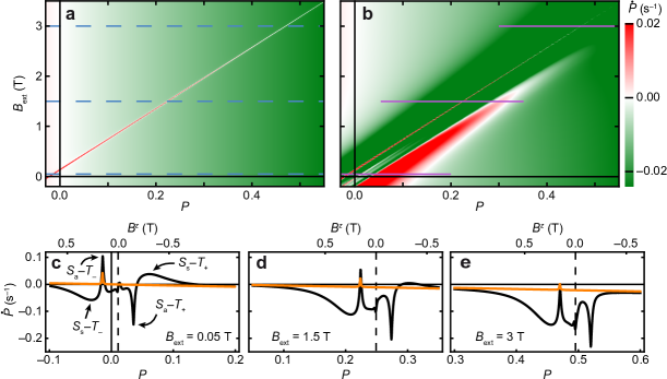
Figure S2: Nuclear polarization rate a) The nuclear polarization rate, $\dot{P}$, calculated analytically using equation (1) of the main article. The dashed horizontal lines correspond to the constant $B_{\text{ext}}$ slices shown in Fig. 3b of the main article. b) $\dot{P}$ calculated numerically using equation (S16) with $\Gamma_{\text{R}}=$4.5\text{\,}\mathrm{GHz}$$ and $N=10^{6}$ nuclei. A random Gaussian distribution was used for $B^{x}_{\text{nuc}}$ and $B^{y}_{\text{nuc}}$ as in reference Jouravlev and Nazarov (2006). The scale bar applies to both a and b. Both calculations were performed using $t_{c}=$12\text{\,}\mathrm{\SIUnitSymbolMicro eV}$$, $\Delta=$8\text{\,}\mathrm{\SIUnitSymbolMicro eV}$$, $\Gamma_{\text{rel}}=$0.04\text{\,}{\mathrm{s}}^{-1}$$, and the magnetic field distribution of the nanomagnet (Fig. 1c, main article). c-d) $\dot{P}$ as a function of $P$ at constant $\mathbf{B}_{\text{ext}}$ (lines in a,b) comparing the rate equation model [orange, equation (1) of the main article] with the perturbation calculation [black, equation (S16)]. The ranges in $P$ of these slices are indicated by the magenta lines in b. The polarization rate extrema associated with the four singlet-triplet resonances are labeled in c. The top axis indicates the $z$-component of the total effective magnetic field, $B^{z}=B_{\text{ext}}+\overline{B}^{z}_{\text{nm}}-PB_{\text{nuc}}^{\text{max}}$. In addition to the extrema associated with the singlet-triplet resonances small polarization features appear near $B^{z}=0$ (dashed vertical lines) where triplets become degenerate.

VI V. Hyperfine- and Non-hyperfine–induced Leakage Current

The leakage current through the DQD shown in Fig. 2b of the main article contains a number of features which can be traced back to the inhomogeneous field produced by the single domain nanomagnet. To illustrate this, in Fig. S3 we show the PSB leakage current through two different DQD devices with identical gate layout. The data in Figs. S3a and S3b show measurements for opposite sweep directions acquired on the sample also presented in the main article but for a larger interdot tunnel coupling $t_{\text{c}}\sim$15\text{\,}\mathrm{\SIUnitSymbolMicro eV}$$. These data are more richly featured compared to those in Fig. S3c in which no nanomagnet was present ($t_{\text{c}}\sim$1\text{\,}\mathrm{\SIUnitSymbolMicro eV}$$).

In Fig. S3c, the measured current is approximately symmetric with respect to the $B_{\text{ext}}=0$ axis, and the main features are increased current along the $\Delta=0$ and $B_{\text{ext}}=0$ axes (for $\Delta\gtrsim 0$, that is, outside of Coulomb blockade) and a global maximum at $\Delta=B_{\text{ext}}\simeq 0$. Similar data have already been published and discussed in detail in reference Koppens et al. (2005). In short, current is created by $t_{\text{c}}$ in combination with the hyperfine interaction, which mixes triplet and singlet states strongly when $\Delta\simeq 0$ or $B_{\text{ext}}\simeq 0$. The width of the current maximum along the $B_{\text{ext}}=0$ axis is determined by the standard deviation of the fluctuating $\mathbf{B}_{\text{nuc}}$Koppens et al. (2005); Jouravlev and Nazarov (2006). The data in Figs. S3a and S3b illustrate that the sizeable $\mathbf{B}_{\text{nm}}$ adds complexity. The following list provides a short explanation for each of the features specific for the sample with nanomagnet:

• The most obvious response to expect when sweeping $B_{\text{ext}}$ is hysteresis of the magnetization of the single domain nanomagnet. Because of its single-domain character, we expect the nanomagnet to switch polarization abruptly when $B_{\text{ext}}$ passes the coercive field. An abrupt switch in magnetic field, in turn, should cause an equally abrupt change in the leakage current signal. Such features are indeed observed in Figs. S3a,b at $B_{\text{ext}}\simeq\mp$52\text{\,}\mathrm{mT}$$, respectively (see white arrows), and are also seen in Fig. 2b of the main article.

• In the presence of $\mathbf{B}_{\text{nm}}$, the eigenenergies of the $T_{\pm}$–like states are never zero. However, the relevant magnetic field, $\left|\mathbf{B}^{\text{L}}+\mathbf{B}^{\text{R}}\right|$ can be minimized by $B_{\text{ext}}$, and at this minimum, the $T_{\pm}$ are most degenerate and a local maximum of the leakage current is expected. For our $\mathbf{B}_{\text{nm}}$ values, $\left|\mathbf{B}^{\text{L}}+\mathbf{B}^{\text{R}}\right|$ is minimized at $B_{\text{ext}}\simeq\pm$12\text{\,}\mathrm{mT}$$, depending on the polarization of the nanomagnet. These fields are indicated in Figs. S3a,b with red arrows and faithfully identify the current maxima.

• The observation of distinct local current maxima at the $S_{\mathrm{a}}$–$T_{\pm}$ resonance (black arrows in Figs. S3a and S3b) and in Fig. 2b of the main article) is unique to samples containing a single domain nanomagnet. The sharpness of these peaks can only be explained by taking into account the hyperfine induced dynamics of the nuclear spins. The actual position of the $S_{\mathrm{a}}$–$T_{\pm}$ resonance is shifted towards larger $\left|B_{\text{ext}}\right|$ compared to its prediction (see Fig. 2b of the main article). In the main article we explain this shift by taking into account the hyperfine induced DNSP.

• $\mathbf{B}_{\text{nm}}$ mixes triplet and singlet states weakening the spin blockade and allowing leakage current to flow. However, $B_{\text{ext}}$ tunes this mixing. In fact, the condition $\Delta\mathbf{B}\parallel\overline{\mathbf{B}}$ defines a local minimum of the singlet mixture with the $T_{\pm}$ states Jouravlev and Nazarov (2006). This can be readily seen from the Hamiltonian in equation (S7) if the quantization axis is chosen parallel to $\overline{\mathbf{B}}$. For our system, this condition is satisfied when $B_{\text{ext}}\simeq\pm$8\text{\,}\mathrm{mT}$$. We actually observe current minima at slightly shifted values (see yellow arrows in Fig. S3a,b) owing to the complex DNSP that occurs while sweeping $B_{\text{ext}}$ (see Fig. S2).

The current at finite $B_{\text{ext}}$ and small $\Delta$ in Figs. S3a and S3b is characterized by strong switching noise and dragging effects which has also been observed in samples without on-chip magnetKoppens et al. (2005); Kobayashi et al. (2011). We forgo a detailed discussion of these effects, which can be explained in terms of the hyperfine dynamics in the presence of more than one stable fixed point at $\Delta\sim 0$Rudner et al. (2011).

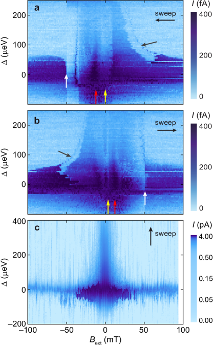
Figure S3: Spin-blockaded leakage current. a) The dc leakage current, $I$, as a function of $B_{\text{ext}}$ (swept from positive to negative) and $\Delta$ (stepped from positive to negative) ($t_{\text{c}}\sim$15\text{\,}\mathrm{\SIUnitSymbolMicro eV}$$. b) Same as in a but for the opposite sweep direction of $\mathbf{B}_{\text{ext}}$ (from negative to positive). Arrows in a and b mark specific features explained in the main text. c) $I$ as a function of $B_{\text{ext}}$ and $\Delta$ measured using a sample with an identical gate layout as the sample used in the main article, but without the on-chip nanomagnet. Overall, maximum $I$ values are one order of magnitude larger than in a and b owing to stronger source/drain coupling with this particular gate tunning, but the region of enhanced $I$ is much smaller. The magnetic field was stepped from right to left and the energy detuning was swept from bottom to top. The perpendicular sweep direction compared to a and b does not affect the main features of this measurement. It does however cause a noisy background which is typical for this sweep direction and is caused by charge noise triggered by sweeping gate voltages.

VII VI. Nuclear Polarization Build-up

Here we present additional data to support our interpretation of the DNSP data. Fig. S4 demonstrates that the polarization dragging in Fig. 4b of the main article is reproducible. All the main features in Fig. S4a are reproducible, especially the position of $B^{\text{max}}_{\text{ext}}$ where polarization is lost. The current measured at the beginning of each field sweep near $B_{\text{ext}}=0$ is the typical leakage current that appears near $B_{\text{ext}}=0$ (see, for example, Fig. S5) and is extended somewhat because of DNSP. We interpret the sharp current maximum (labeled $B_{\text{ext}}^{\text{max}}$) as the point of maximum polarization (see main article). The $\delta I$ in Fig. S4b results from losing the stable polarization condition and related resonant current as the polarization decays and the system drifts away from resonance.

Fig. S5 shows a second technique for demonstrating the polarization created during fixed-point dragging measurements. In Fig. S5a, we show $I$ measured as a function of $B_{\text{ext}}$ and $\Delta$ over a much larger range of $B_{\text{ext}}$ than Fig. 2b of the main article. The current features at low $B_{\text{ext}}$ in S5a differ from those in Fig. 2b of the main article mostly because $\Delta$ was swept rather than $B_{\text{ext}}$.

The current traces in Fig. S5b, measured at $B_{\text{ext}}=$250\text{\,}\mathrm{mT}$$ after the nuclei have been polarized to $P\approx$4\text{\,}\mathrm{\char 37\relax}$$, are very similar to the trace in Fig. S5c, which shows current measured at $B_{\text{ext}}=$17.5\text{\,}\mathrm{mT}$$ and $P=$0\text{\,}\mathrm{\char 37\relax}$$. The quantitative similarity between the $P\approx$4\text{\,}\mathrm{\char 37\relax}$$ current traces in Fig. S5b and the trace in Fig. S5c allows us to conclude that $B^{z}_{\text{nuc}}$ compensates $B_{\text{ext}}$ ($B^{z}_{\text{nuc}}\simeq-B_{\text{ext}}$ for $B_{\text{ext}}\gg\left|\mathbf{B}_{\text{nm}}\right|$) thereby reducing the total effective field. In contrast to the polarized traces in Fig. S5b, which are almost symmetric with respect to $\Delta=0$, the $P=$0\text{\,}\mathrm{\char 37\relax}$$ curve in Fig. S5c is asymmetric and exhibits switching noise for $\Delta>0$. We attribute this behavior to small changes in nuclear spin polarization, while in Fig. S5b, the polarization is stabilized at the adjustable fixed point (A-FP). The current traces in Fig. S5b measured at $P\approx$4\text{\,}\mathrm{\char 37\relax}$$ are repeatable and much larger than the trace measured at $P=$0\text{\,}\mathrm{\char 37\relax}$$. This demonstrates that the polarization is finite and stable.

Current features, such as the local maxima in Fig. 2a of the main article and Fig. S4 at $B_{\text{ext}}>1\,$T, are not seen in Fig. S5a. These features are missing because $\Delta$ is swept, and significant polarizations are not obtained. Taken together with Figs. 2,3 of the main article, Figs. S4 and S5 demonstrate the ability of our system to generate large nuclear spin polarization—and detect it.

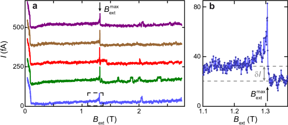
Figure S4: Polarization sweep repeatability a) Five polarization sweeps measured at a rate $\dot{B}_{\text{ext}}=$35\text{\,}\mathrm{mT}\text{/}\mathrm{min}$$ and $\Delta=$150\text{\,}\mathrm{\SIUnitSymbolMicro eV}$$. The traces are offset by $N\times$120\text{\,}\mathrm{fA}$;N=0,1,2,3,4$ for clarity. The current bistabilities observed beyond $B^{\text{max}}_{\text{ext}}$ are consistent with DNSPKoppens et al. (2005); Rudner et al. (2011). b) The details of a current trace near $B^{\text{max}}_{\text{ext}}$ taken from within the boxed region of a demonstrate a sharp resonance and clear change in current, $\delta I\simeq$11\text{\,}\mathrm{fA}$$, before and after sweeping through $B^{\text{max}}_{\text{ext}}$.

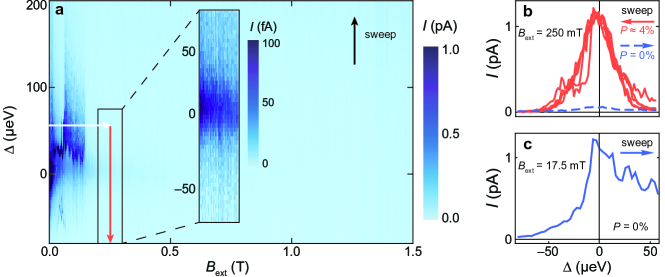
Figure S5: PSB leakage current at large $B_{\text{ext}}$ a) Leakage current, $I$, as a function of $\Delta$ and a large range of $B_{\text{ext}}$. The magnetic field has been stepped and $\Delta$ has been swept from negative to positive to minimize DNSP effects. Inset: Enlarged region centered at $B_{\text{ext}}=$250\text{\,}\mathrm{mT}$$ showing the small ($\sim$100\text{\,}\mathrm{fA}$$) leakage current when $P=$0\text{\,}\mathrm{\char 37\relax}$$. b) The solid orange lines are $I$ measured while sweeping $\Delta$ multiple times through $\Delta=0$ into Coulomb blockade along the orange arrow in a. These data were measured after ramping $B_{\text{ext}}$ from $B_{\text{ext}}\simeq 0$ to $B_{\text{ext}}\simeq$250\text{\,}\mathrm{mT}$$ (along the white arrow in a) creating a polarization of $P\simeq$4\text{\,}\mathrm{\char 37\relax}$$. The dashed blue line is $I$ at $P=$0\text{\,}\mathrm{\char 37\relax}$$ extracted from a at $B_{\text{ext}}=$250\text{\,}\mathrm{mT}$$ and is negligible compared to $I$ with polarization. c) $I$ measured versus $\Delta$ starting with unpolarized nuclei extracted from a at $B_{\text{ext}}=$17.5\text{\,}\mathrm{mT}$$.

VIII VII. Data Fitting

The fitting procedure of the data in article Figs. 2b and 3a involves solving numerically the nonlinear differential equation given by equation (1) of the main article for a given set of parameters. This produces $P(t)$, which is then fed into equation (2) to find $I(t)$. Our goal is not to reproduce the details of the measured $I(t)$ traces, but only the position of its maximum at the $S_{\text{a}}$–$T_{-}$ resonance, that is, the position of the resonant current $I_{\text{max}}$. Therefore, the final step is to calculate the position of $I_{\text{max}}$ using the numerical $I(t)$. This procedure was repeated with different parameter sets until an agreement between theory and data was found.

The numerical fit needs the following parameters: $t_{\text{c}}$, $\gamma$, $\alpha$, $I_{\text{max}}$, and $\Gamma_{\text{rel}}$ (see equations (1–3) of the main article). $I_{\text{max}}$ and the ratio $\alpha/\Gamma_{\text{rel}}=$0.8\text{\,}{\mathrm{pA}}^{-1}$$ (see main article Fig. 4d) were measured, thus reducing the overall number of fit parameters to three.

For the time-dependent data (see main article Figs. 3), $I_{\text{max}}=$100\text{\,}\mathrm{fA}$$ is the measured peak height. $I_{\text{max}}$ values for the $\Delta$-dependent data (see main article Fig. 2b) are unique for each value of $\Delta$ because $I$ is $\Delta$ dependent. Fig. S6 details how $I_{\text{max}}(\Delta)$ is extracted from the $I$ measured as a function of $B_{\text{ext}}$ and $\Delta$. The main result is that $I_{\text{max}}(\Delta)$ is identical to $I(\Delta)$ measured near $B_{\text{ext}}=0$, where spin blockade is lifted.

When $\mathbf{B}_{\text{nm}}$ and $\mathbf{B}_{\text{nuc}}$ are known, the $\Delta$–$B_{\text{ext}}$ position of the $S_{\text{a}}$–$T_{-}$ resonance can be approximated analytically. This approximation is used in equation (4) of the main article and includes only $B^{z}_{\text{nm}}$ providing $E_{\text{z}}^{\pm}\simeq\pm g\mu_{\text{B}}\left(B_{\text{ext}}-B^{\text{max}}_{\text{nuc}}P+\overline{B}^{z}_{\text{nm}}\right)$. In Fig. S7, we compare exact numerical results with the analytical approximations for all four singlet–triplet resonances. The analytical approximation for the $S_{\text{a}}$–$T_{-}$ resonance is in excellent agreement with the numerical calculation for $B_{\text{ext}}\geq 0$.

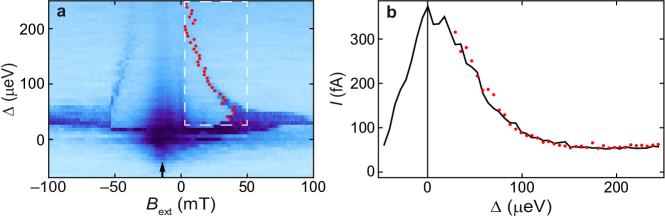
Figure S6: Determination of $I_{\text{max}}$. a) Leakage current, $I$, measured versus $B_{\text{ext}}$ and $\Delta$ repeated from Fig. 2b of the main article. After searching within the boxed region, the $\CIRCLE$ indicate the $B_{\text{ext}}$-$\Delta$ position of $I_{\text{max}}$ along the $S_{\text{a}}$–$T_{-}$ resonance. b) Here $\CIRCLE$ are the $I_{\text{max}}$ values from a plotted as a function of $\Delta$. In comparison, the black line is $I$ measured versus $\Delta$ along the symmetry axis (black arrow in a). As expected, $I_{\text{max}}(\Delta)$ along the $S_{\text{a}}$–$T_{-}$ resonance follows the general $I(\Delta)$ trend. A smoothed version of $I(\Delta)$ is used to create the smooth numerical fit in Fig. 2b of the main article.

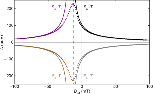
Figure S7: Location of singlet–triplet resonances. The numerically calculated data points indicate the position in the $B_{\text{ext}}$–$\Delta$ plane where singlet and triplet states are resonant. The solid lines are approximated values calculated analytically. Each line is labeled to identify which states are resonant. In particular, the black line is the analytic approximation for the $S_{\text{a}}$–$T_{-}$ resonance and was used to fit the DNSP data (see Fig. 2 of the main article). The exact and approximate values are in excellent agreement for $B_{\text{ext}}\geq 0$, where all DNSP measurements were performed. The upper branch of the numerical calculation is included in Fig. 2b of the main article. The vertical dashed line at $B_{\text{ext}}=$-12\text{\,}\mathrm{mT}$$, which is the minimizing value of $\left|\mathbf{B}^{\text{L}}+\mathbf{B}^{\text{R}}\right|$, defines the symmetry axis where the triplets are most degenerate. Here $t_{\text{c}}=$12\text{\,}\mathrm{\SIUnitSymbolMicro eV}$$.

One set of fit parameters ($t_{\text{c}}=$12\text{\,}\mathrm{\SIUnitSymbolMicro eV}$$, $\Gamma_{\text{rel}}=$0.043\text{\,}{\mathrm{s}}^{-1}$$, $\gamma=$10\pm 1.\text{\,}\mathrm{mT}$$, and $\alpha=$35\text{\,}{\mathrm{nA}}^{-1}\text{\,}{\mathrm{s}}^{-1}$$) reproduces the data of two very different experiments in Figs. 2b,3a of the main text. The data sets were measured using identical gate voltages. For a slightly different system tuning, only two parameters are expected to change, namely $t_{\text{c}}$ and $\alpha$, because they reflect the various hyperfine and non-hyperfine system rates, which are strongly gate dependent. $\gamma$ depends mostly on $\mathbf{B}_{\text{nm}}$, which is constant, while $\Gamma_{\text{rel}}$ should be independent of gate tuning because it is a property of the nuclei. These expectations are supported in Fig. S8 where $I$ versus $B_{\text{ext}}$ and time has been measured after making the voltage of the top center gate more positive (see the gate design in Fig. 1a of the main article). The ability to describe disparate sets of data in different tuning regimes with either no change or only justifiable adjustments to fit parameters demonstrates the validity of our model.

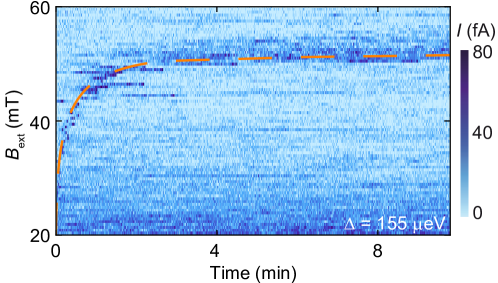
Figure S8: Nuclear Spin Dynamics. Current measured as a function of time demonstrating DNSP at the $S_{\text{a}}$–$T_{-}$ resonance. The dashed orange line is a numerical fit of the data. Here the system is tuned to a larger tunnel coupling compared to the tuning used in Fig. 3 of the main article. As a result, $t_{\text{c}}=$22\text{\,}\mathrm{\SIUnitSymbolMicro eV}$$ is larger, which makes $E_{\text{a}}$ larger, and the current peak is not observed until $B_{\text{ext}}\approx$20\text{\,}\mathrm{mT}$$. Meanwhile, $\alpha=$14\text{\,}{\mathrm{nA}}^{-1}\text{\,}{\mathrm{s}}^{-1}$$ suffers from the increased $t_{\text{c}}$. The other fit parameters are unchanged, that is, $\gamma=$10\text{\,}\mathrm{mT}$$ and $\Gamma_{\text{rel}}=$0.04\text{\,}{\mathrm{s}}^{-1}$$.

References

Kane (1998)B. E. Kane, Nature 393, 133 (1998).
Jelezko and Wrachtrup (2006)F. Jelezko and J. Wrachtrup, Physica Status Solidi A 203, 3207 (2006).
Kou et al. (2010)A. Kou, D. T. McClure,
C. M. Marcus, L. N. Pfeiffer, and K. W. West, Phys. Rev. Lett. 105, 056804 (2010).
Urbaszek et al. (2012)B. Urbaszek, X. Marie,
T. Amand, O. Krebs, P. Voisin, P. Maletinsky, A. Hogele, and A. Imamoglu, ArXiv e-prints arXiv:1202.4637v2 [cond-mat.mes-hall] (2012).
Schliemann et al. (2003)J. Schliemann, A. Khaetskii, and D. Loss, J.
Phys.-Condes. Matter 15, R1809 (2003).
Fischer et al. (2009)J. Fischer, M. Trif,
W. A. Coish, and D. Loss, Solid State Commun 149, 1443 (2009).
Yao et al. (2006)W. Yao, R. B. Liu, and L. J. Sham, Phys. Rev. B 74, 195301 (2006).
Cywinski et al. (2009)L. Cywinski, W. M. Witzel, and S. Das Sarma, Phys. Rev. Lett. 102, 057601 (2009).
Bluhm et al. (2011)H. Bluhm, S. Foletti,
I. Neder, M. Rudner, D. Mahalu, V. Umansky, and A. Yacoby, Nature Phys. 7, 109 (2011).
Laird et al. (2007)E. A. Laird, C. Barthel,
E. I. Rashba, C. M. Marcus, M. P. Hanson, and A. C. Gossard, Phys. Rev. Lett. 99, 246601 (2007).
Petta et al. (2008)J. R. Petta, J. M. Taylor,
A. C. Johnson, A. Yacoby, M. D. Lukin, C. M. Marcus, M. P. Hanson, and A. C. Gossard, Phys. Rev. Lett. 100, 067601 (2008).
Foletti et al. (2009)S. Foletti, H. Bluhm,
D. Mahalu, V. Umansky, and A. Yacoby, Nature Phys. 5, 903 (2009).
Reilly et al. (2010)D. J. Reilly, J. M. Taylor,
J. R. Petta, C. M. Marcus, M. P. Hanson, and A. C. Gossard, Phys. Rev. Lett. 104, 236802 (2010).
Burkard et al. (1999)G. Burkard, D. Loss, and D. P. DiVincenzo, Phys. Rev. B 59, 2070 (1999).
Klauser et al. (2006)D. Klauser, W. A. Coish,
and D. Loss, Phys. Rev. B 73, 205302 (2006).
Rudner and Levitov (2007)M. S. Rudner and L. S. Levitov, Phys.
Rev. Lett. 99, 036602
(2007).
Danon and Nazarov (2008)J. Danon and Y. V. Nazarov, Phys.
Rev. Lett. 100, 056603
(2008).
Latta et al. (2009)C. Latta, A. Högele,
Y. Zhao, A. N. Vamivakas, P. Maletinsky, M. Kroner, J. Dreiser, I. Carusotto, A. Badolato, D. Schuh, W. Wegscheider, M. Atature, and A. Imamoglu, Nature Phys. 5, 758 (2009).
Vink et al. (2009)I. T. Vink, K. C. Nowack,
F. H. L. Koppens,
J. Danon, Y. V. Nazarov, and L. M. K. Vandersypen, Nature Phys. 5, 764 (2009).
Danon et al. (2009)J. Danon, I. T. Vink,
F. H. L. Koppens,
K. C. Nowack, L. M. K. Vandersypen, and Y. V. Nazarov, Phys. Rev. Lett. 103, 046601 (2009).
Bluhm et al. (2010)H. Bluhm, S. Foletti,
D. Mahalu, V. Umansky, and A. Yacoby, Phys. Rev. Lett. 105, 216803 (2010).
Sun et al. (2012)B. Sun, W. Yao, X. D. Xu, A. S. Bracker, D. Gammon, L. J. Sham, and D. Steel, J Opt Soc Am B 29, A119 (2012).
Taylor et al. (2003)J. M. Taylor, A. Imamoglu, and M. D. Lukin, Phys. Rev. Lett. 91, 246802 (2003).
Kurucz et al. (2009)Z. Kurucz, M. W. Sorensen, J. M. Taylor, M. D. Lukin, and M. Fleischhauer, Phys. Rev. Lett. 103, 010502 (2009).
Maurer et al. (2012)P. C. Maurer, G. Kucsko,
C. Latta, L. Jiang, N. Y. Yao, S. D. Bennett, F. Pastawski, D. Hunger, N. Chisholm, M. Markham, D. J. Twitchen, J. I. Cirac, and M. D. Lukin, Science 336, 1283 (2012).
Steger et al. (2012)M. Steger, K. Saeedi,
M. L. W. Thewalt,
J. J. L. Morton, H. Riemann, N. V. Abrosimov, P. Becker, and H. J. Pohl, Science 336, 1280 (2012).
Engel-Herbert and Hesjedal (2005)R. Engel-Herbert and T. Hesjedal, J.
Appl. Phys. 97, 074504
(2005).
Ono et al. (2002)K. Ono, D. G. Austing,
Y. Tokura, and S. Tarucha, Science 297, 1313 (2002).
Pioro-Ladriere et al. (2008)M. Pioro-Ladriere, T. Obata, Y. Tokura,
Y. S. Shin, T. Kubo, K. Yoshida, T. Taniyama, and S. Tarucha, Nature Phys. 4, 776 (2008).
Obata et al. (2010)T. Obata, M. Pioro-Ladriere, Y. Tokura, Y. S. Shin,
T. Kubo, K. Yoshida, T. Taniyama, and S. Tarucha, Phys. Rev. B 81, 085317 (2010).
Brunner et al. (2011)R. Brunner, Y. S. Shin,
T. Obata, M. Pioro-Ladriere, T. Kubo, K. Yoshida, T. Taniyama, Y. Tokura, and S. Tarucha, Phys. Rev. Lett. 107, 146801 (2011).
Heedt et al. (2012)S. Heedt, C. Morgan,
K. Weis, D. E. Bürgler, R. Calarco, H. Hardtdegen, D. Grützmacher, and T. Schäpers, Nano. Lett. 12, 4437 (2012).
(33)See attached Supplementary Material for additional information.
Koppens et al. (2005)F. H. L. Koppens, J. A. Folk, J. M. Elzerman, R. Hanson,
L. H. W. van Beveren,
I. T. Vink, H. P. Tranitz, W. Wegscheider, L. P. Kouwenhoven, and L. M. K. Vandersypen, Science 309, 1346 (2005).
Ono and Tarucha (2004)K. Ono and S. Tarucha, Phys. Rev. Lett. 92, 256803 (2004).
Kobayashi et al. (2011)T. Kobayashi, K. Hitachi,
S. Sasaki, and K. Muraki, Phys. Rev. Lett. 107, 216802 (2011).
Frolov et al. (2012)S. M. Frolov, J. Danon,
S. Nadj-Perge, K. Zuo, J. W. W. van Tilburg, V. S. Pribiag, J. W. G. van den Berg, E. P. A. M. Bakkers, and L. P. Kouwenhoven, Phys. Rev. Lett. 109, 236805 (2012).
Rudner et al. (2011a)M. S. Rudner, F. H. L. Koppens, J. A. Folk,
L. M. K. Vandersypen, and L. S. Levitov, Phys. Rev. B 84, 075339 (2011a).
Baugh et al. (2007)J. Baugh, Y. Kitamura,
K. Ono, and S. Tarucha, Phys. Rev. Lett. 99, 096804 (2007).
Giedke et al. (2006)G. Giedke, J. M. Taylor,
D. D’Alessandro, M. D. Lukin, and A. Imamoglu, Phys Rev A 74, 032316 (2006).
Reilly et al. (2008)D. J. Reilly, J. M. Taylor,
J. R. Petta, C. M. Marcus, M. P. Hanson, and A. C. Gossard, Science 321, 817 (2008).
Issler et al. (2010)M. Issler, E. M. Kessler,
G. Giedke, S. Yelin, I. Cirac, M. D. Lukin, and A. Imamoglu, Phys. Rev. Lett. 105, 267202 (2010).
Rudner et al. (2011b)M. S. Rudner, L. M. K. Vandersypen, V. Vuletic, and L. S. Levitov, Phys.
Rev. Lett. 107, 206806
(2011b).
Gullans et al. (2010)M. Gullans, J. J. Krich,
J. M. Taylor, H. Bluhm, B. I. Halperin, C. M. Marcus, M. Stopa, A. Yacoby, and M. D. Lukin, Phys. Rev. Lett. 104, 226807 (2010).
Rudner and Levitov (2010)M. S. Rudner and L. S. Levitov, Phys.
Rev. B 82, 155418
(2010).
Schuetz et al. (2012)M. J. A. Schuetz, E. M. Kessler, J. I. Cirac, and G. Giedke, Phys. Rev. B 86, 085322 (2012).

References

Johnson et al. (2005)RA. C. Johnson, J. R. Petta,
C. M. Marcus, M. P. Hanson, and A. C. Gossard, RPhys. Rev. B 72, 165308 (2005).
Coish and Baugh (2009)RW. A. Coish and J. Baugh, RPhys Status Solidi
B 246, 2203 (2009).
Overhauser (1953)RA. W. Overhauser, RPhys. Rev. 92, 411
(1953).
Rudner et al. (2011)RM. S. Rudner, F. H. L. Koppens, J. A. Folk,
L. M. K. Vandersypen, and L. S. Levitov, RPhys. Rev. B 84, 075339 (2011).
Jouravlev and Nazarov (2006)RO. N. Jouravlev and Y. V. Nazarov, RPhys.
Rev. Lett. 96, 176804
(2006).
Koppens et al. (2005)RF. H. L. Koppens, J. A. Folk, J. M. Elzerman, R. Hanson,
L. H. W. van Beveren,
I. T. Vink, H. P. Tranitz, W. Wegscheider, L. P. Kouwenhoven, and L. M. K. Vandersypen, RScience 309, 1346 (2005).
Kobayashi et al. (2011)RT. Kobayashi, K. Hitachi,
S. Sasaki, and K. Muraki, RPhys. Rev. Lett. 107, 216802 (2011).
.
The (blue) single-domain Co nanomagnet (200 (width) 50 (height) , visible) generates an inhomogeneous magnetic field, .
(b)
The tunneling sequence . Triplet-singlet transitions require lifting of the PSB.
(c) The relevant layers of the heterostructure, gates, and nanomagnet. The magnetic field lines (blue) are calculated according to ref. 27.
The black arrows indicate the local magnetic fields and . The radius of
.
The (blue) single-domain Co nanomagnet (200 (width) 50 (height) , visible) generates an inhomogeneous magnetic field, .
(b)
The tunneling sequence . Triplet-singlet transitions require lifting of the PSB.
(c) The relevant layers of the heterostructure, gates, and nanomagnet. The magnetic field lines (blue) are calculated according to ref. 27.
The black arrows indicate the local magnetic fields and . The radius of  represents the typical Overhauser field fluctuations.