Optimal design of dilution experiments under volume constraints

Abstract

The paper develops methods to construct a one-stage optimal design of dilution experiments under the total available volume constraint typical for bio-medical applications. We consider various design criteria based on the Fisher information both is Bayesian and non-Bayasian settings and show that the optimal design is typically one-atomic meaning that all the dilutions should be of the same size. The main tool is variational analysis of functions of a measure and the corresponding steepest descent type numerical methods. Our approach is generic in the sense that it allows for inclusion of additional constraints and cost components, like the cost of materials and of the experiment itself.

Keywords: Dilution experiment, optimal design of experiments, Fisher information criteria, gradient methods, design measure, variational analysis on measures, stem cells counting.

AMS 1991 Subject Classification. Primary: 62K05; Secondary: 62F15, 62F30, 65K10, 49K45

1 Introduction

The paper studies a wide class of statistical experiments with the total volume constraint arising, in particular, in stem cells research, a very active area of experimental biology. Stem cells are the cells produced during early stages of embryonic development and they are having capacity to turn into various types of tissue cells. This potentially opens new ways to cure many diseases and explains the huge importance of the stem cells research, see, e. g., Mayhall:2004 and the references therein. We aim to characterise an optimal design of dilution-type experiments under the contraint of the available solution which is typical for experiments involving counting stem cells. Specifically, this study originates in studies of Hematopoietic or blood stem cells (HSCs) which are the stem cells giving rise to all red and white blood cells and platelets. HSCs develop in a mammal’s embryo in early days from cells. There is not much known on the biological mechanism which triggers a cell to develop into an HSC and there is no direct way so far to observe such cells, called pre-HSCs, which soon to become HSCs. Pre-HSCs are mostly produced in aorta-gonad-mesonephros (AGM) region of the embryonic mesoderm and also in the yolk sac, then colonise the liver. A challenging problem is how to detect the pre-HSCs and how many of them are present at a different embryo ages.

In order to estimate the number of pre-HSCs present in a given region, experiments on laboratory mice have been conducted which use the following signature property of stem cells. A mature HSC is capable to cure a mouse which receives a controlled dose of radiation if injected in its blood. A mouse recovers (repopulates), if and only if, it has received at least one HSC in the injected dose. Thus the number of pre-HSCs can be estimated by the so-called limiting dilution method: controlled dozes of a substrate containing samples from the AGM are injected into irradiated mice and then the number of repopulated mice infers on the number of HSCs which developed from the initially present pre-HSCs.

The dilution method has been in the arsenal of biologists for almost a century, at least since McCrady used it for quantitative determination of Bacillus coli in water in 1915, McCrady:1915. Since then many studies used it to estimate the number of objects of interest in a medium without their direct count, Fisher:1922, Cochran:1950, Ridout:1995, to name a few.

So far, several studies have produced estimates for the number of pre-HSCs in AGM by using the dilution method which varies between just a few to, perhaps, as many as 200, see, e. g., Kumaravelu:2002, Gekas:2005, Ottersbach:2005 Bonne:2010 and Medvinsky:2011. Most of the reports tend to focus on the modelling of experimental data and on the estimation methods. However, there has been little discussions on how to design the experiment to capture the most informative sample. Indeed, the experiment would be spoilt, if all the mice repopulate or if all do not. The aim of this paper is to find an optimal design of the dilution experiment to estimate the mean number of pre-HSCs. What distinguishes the experiments we are dealing with in this paper from other dilution experiments extensively covered in statistical literature are the following two features. First, it is the volume contraint imposed by the limited size of available substrate from AGMs. Second, a significant time delay between the dose injection and the result of its action prevents from using multi-stage designs when the further stages of experiments are based on the outcomes of the previous one(s). To address these specific issues, we employ recently developed methods of constrained optimisation of functionals of measures and the corresponding steepest descent type algorithms for computations. It should be stressed that our methodology is generic in the sense that it can be applied to other dilution experiments and not only in the stem cells research. Moreover, additional contraints can be incorporated into the model which would allow, for instance, to take into account the cost of mice or other materials used in the experiment.

This study is organised in the following way. Section 2 introduces the dilution experiment we are dealing with, description of the corresponding statistical model followed by its assumptions, and at the end the optimality criterion functions. Section 3 lays out the theoretical basis for the optimisation methods we are using given that the goal functions are represented as functions of a measure. Consecutive sections provide the optimal design of the dilution experiments under various conditions and various goal functions: in non-Bayesian setting in Section 4.1, then under Uniform and Gamma Bayesian priors in Section 4.2, and finally in Section 4.3 we represent an optimal design that integrates cost to the criterion functions. We conclude by discussion of our findings and their extensions in Section 5.

2 Dilution experiment, statistical model and optimality criteria

Description of experiment

The dilution experiment on estimation of the number of HSCs we address here involved the AGM region of an 11 days old mouse embryo. More exactly, in order to make a study more representable and not depending on features of a particular embryo, an engineered AGM is made from several such embryos. A substrate of volume $V$ is then made from this engineered AGM and the content is thoroughly mixed. Next, $n$ doses containing proportions $x_{1},\dotsc,x_{n}$ of the whole $V$ are extracted from all or part of the substrate and left for a few days so that pre-HSCs in these doses, if any, mature into HSCs. Finally, these $n$ doses are injected into $n$ irradiated mice (the number $n$ of mice was 30 in this experiment) so that each mouse receives its own dose and the mice are put to rest for a few weeks for the doses to take effect. After this, the number of repopulated mice, which are the ones having received a doze with at least one pre-HSC, is counted and the inference is drawn on the total number of pre-HSCs initially present in the AGM. The main question to address when designing such an experiment is doses of which volumes should be used for available number of mice in order to get best possible quality of the statistical estimator? Different criteria could be considered to quantify the quality of the estimator. We will consider below most common ones based on the Fisher information.

Statistical model

Given the description of the experiment above, the following assumptions can be made.

• Spatial homogeneity: pre-HSCs were distributed uniformly throughout the substrate when the doses were taken. Thus there is no tendency for pairs or groups of pre-HSCs either to cluster or to reject one another. This is implied by the fact that the substrate was thoroughly mixed just before the doses are taken.

• Orderliness: the probability that there are more than one pre-HSCs in a small volume $dv$ of substrate has order $o(dv)$. This is a natural assumption given that an 11 days old AGM contains about 300 thousand cells and only no more than 200 of these are pre-HSCs.

• Independence: each cell in substrate has the same (small) probability to turn into a pre-HSC independently of the other cells.

• Only a pre-HSC can develop into a mature HSC. So that a dose contains at least one HSC at the time of injection to a mouse if and only if there was a pre-HSC present in the dose at the time of its extraction from the whole substrate.

• Finally, each dose when injected into an irradiated mouse is certain to exhibit a positive result (repopulated mouse), whenever the dose contains at least one HSC.

The first three assumptions above suggest that the locations of pre-HSCs in the substrate $V$ are given by a homogeneous Poisson point process. This follows from the Poisson limit theorem for thinned point processes, see, e. g.,  [Sec. 11.3]DalVJon:08. Indeed, in every subset of the substrate of a positive volume $x$, the number of cells turned into pre-HSCs is well approximated by the Poisson distribution with the parameter proportional to the mean number of pre-HSCs in the substrate which is $\lambda x$ for some parameter $\lambda>0$. Because of the independence assumption, these numbers are independent for disjoint subsets. Changing the units if necessary, we assume from now on that the volume of the whole substrate is 1. The parameter $\lambda$ is then the unknown density of the Poisson point process which is also the mean number of pre-HSCs in the substrate. Thus we operate with a measurable space carrying point configurations inside a set $V\subset\mathbb{R}^{3}$ of volume 1 (the space of finite counting measures $\omega$ on $V$ with the minimal $\sigma$-algebra making the mappings $\omega\mapsto\omega(B)$ measurable for all Borel $B\subseteq V$) supplied with probability distribution $\mathbf{P}_{\lambda}$ so that $\omega$ under $\mathbf{P}_{\lambda}$ is a homogeneous Poisson point process with density $\lambda$.

The doses taken can now be associated with disjoint subsets $V_{1},\dotsc,V_{n}$ of $V$ with volumes $x_{i}>0$, $i=1,\dotsc,n$. The corresponding numbers of pre-HSCs $\omega(V_{i}),\ i=1,\dotsc,n$ in the doses are then independent Poisson distributed random variables with parameters $\lambda x_{i}$ while the total number of pre-HSCs $\omega(V)$ is Poisson distributed with parameter $\lambda$.

In the simplest case all the doses have the same volume $0<x\leq 1/n$. The probability that a doze is sterile, i.e. it does not contain a pre-HSC, is then

$$p=\mathbf{P}\{\omega(V_{i})=0\}=e^{-\lambda x}.$$ (1)

Thus the total number of non-repopulated mice follows Binomial distribution with parameters $n,p$ and the maximum likelihood estimate for the average number of HSC $\lambda$ is given by

$$\hat{\lambda}=-\frac{\log\hat{p}}{x},$$ (2)

where $\hat{p}$ is the proportion of non-repopulated mice provided it is not 0. However, the doses need not be necessarily all equal for an optimal design.

Let $\chi_{i}$ ($i=1,...,n$) be an indicator that a mouse, which received the $i$th dose of volume $x_{i}$, has not repopulated. Thus, $\chi_{i}$ is a Bernoulli random variable

$${\chi_{i}}|{\lambda}\sim\operatorname{Bern}({e^{-\lambda x_{i}}})$$ (3)

with the parameter equal to the probability of the $i$th dose to be sterile.

Hence, the log-likelihood function for the sequence $\bm{\chi}=(\chi_{1},...,\chi_{n})$ of non-repopulated and repopulated mice is given by

$$\ell(\bm{\chi}\mid\lambda,\mathbf{x})=-\sum_{i=1}^{n}\chi_{i}\lambda x_{i}+\sum_{i=1}^{n}(1-\chi_{i})\log(1-e^{-\lambda x_{i}}),$$ (4)

where $\mathbf{x}=(x_{1},...,x_{n})$. Maximisation of this expression over $\lambda$ for an observed sample $\bm{\chi}$ provides a maximum likelihood estimator (MLE) of $\lambda$ for a given design $\mathbf{x}$. Our goal here is to determine the optimal design in terms of the doses $\{x_{i}\}$, according to a suitably chosen optimality criterion, which we describe next.

Optimality criterion functions

Recall that for a statistical model which depends on a one-dimensional parameter $\lambda$, the Fisher information is defined as

$$I(\mathbf{x};\lambda)=-\operatorname{{\bf E}}_{\lambda}\biggl{[}\frac{\partial^{2}\ell(\bm{\chi}|\lambda,\mathbf{x})}{\partial\lambda^{2}}\biggr{]}.$$ (5)

The expectation $\operatorname{{\bf E}}_{\lambda}$ is taken here w.r.t the random vector $\bm{\chi}$.

Derived from (4), we have in our case

$$I(\mathbf{x};\lambda)=\sum_{i=1}^{n}\frac{e^{-\lambda x_{i}}}{1-e^{-\lambda x_{i}}}x_{i}^{2}.$$ (6)

The Fisher information measures the amount of information that an observable sample carries about the unknown parameter, which the likelihood function depends upon. On the other hand, it is the inverse of MLE’s variance, see, e. g.,  Everitt:2010. Thus, maximising the information corresponds to minimising the variance of the MLE. Therefore, maximising the Fisher information (6) over $\mathbf{x}$ under constraint $\sum_{i=1}^{n}x_{i}\leq 1$ is a useful design criterion.

It is typical in statistical experiment planning to describe design in term of a probabilistic design measure. Typically, the design measure is atomic, so it has a form $\sum_{j}q_{j}\delta_{x_{j}}$, where $\delta_{x}$ is the unit mass measure concentrated on a point $\{x\}$. The design measure reflects the (asymptotic when $n\to\infty$) frequency $q_{j}$ of occurrence of the value $x_{j}$ in the design, see, e. g.,  atk:don92. By this reason, we will also describe the doses by a measure $\mu(dx)$ living on $(0,1]$, albeit not renormalised to have mass 1. Namely, $\mu=\sum_{j}m_{j}\delta_{x_{j}}$ means the design when a dose of volume $x_{j}$ is repeated $m_{j}$ times. Since it is senseless for an experiment involving estimation of $\lambda$ to give a mouse zero-doze of the substrate, we exclude the point 0 from the design space. Obviously, we have that the total mass constraint $\sum_{j=1}^{k}m_{j}=\int\mu(dx)=n$ and that we cannot extract more doses than the total volume of the substrate: $\sum_{j=1}^{k}m_{j}x_{j}=\int x\mu(dx)\leq 1$. All integrals here and below are taken over $(0,1]$, unless specified differently.

Now the basic optimisation problem for the design of our experiment is

$$G_{1}(\mu;\lambda) =I(\mu;\lambda)=\int\frac{e^{-\lambda x}}{1-e^{-\lambda x}}x^{2}\,\mu(dx)\to\sup$$ (7)

over measures $$\mu \operatorname{supp}\mu\subseteq[0,1]$$ with support satisfying

$$\mu(\{0\})=0;$$

$$\mu((0,1])=n;$$ (8)

$$\int x\,\mu(dx)\leq 1.$$ (9)

A design measure describes asymptotic frequencies, so $q_{j}n=m_{j}$ for a given finite $n$ may not be all integers. In this case it is reasonable to consider the nearest measure with all $m_{j}\in\mathbb{Z}_{+}$ as an approximation to the optimal solution. Or, if necessary, a choice of the optimal measure among such measures can be done by evaluation of the goal function at just a few closest approximations of this kind to the optimal design measure.

Bayesian setting

Sometimes, there is an additional information available on the plausible values of the parameter $\lambda$ which is given in a form of a prior distribution $Q(d\lambda)$, see, e. g.,  [Sec. 2.2.2]Mar:Rob07. In this case the optimality criterion involves taking the expectation of the goal functions w.r.t the distribution $Q$.

For a single parameter, the following criterion functions are typically used to find an optimal design, see, e.g., atk:don92 or Ridout:1995:

$$G_{2}(\mu)=\operatorname{{\bf E}}_{Q}I(\mu;\lambda)$$ (10)

$$G_{3}(\mu)=\operatorname{{\bf E}}_{Q}\log I(\mu;\lambda)$$ (11)

$$G_{4}(\mu)=-\operatorname{{\bf E}}_{Q}\bigl{(}I(\mu;\lambda)\bigr{)}^{-1}$$ (12)

Criterion function $G_{2}$ and $G_{3}$ maximize, under the same constraints (8) and (9), the expectation of the Fisher information and of its logarithm, respectively, as used in e.g., in za:77 and ch:la89. The criterion function $G_{4}$ minimises the expected asymptotic variance of the maximum likelihood estimator.

Next section will describe a general framework of optimisation of functionals of measures and the recently developed techniques for solving such optimisation problems. Apart from optimal design of statistical experiments Pukelsheim:83, atk:don92, these are frequent in different subjects, like spline approximation of curves and geometrical bodies where the measure describes the positions of spline points Schneider:88, maximisation the area covered by random geometric objects with the distribution determined by a measure Hall:88, stochastic search, where a measure determines the search strategy WZ:94, Z:91.

3 Optimisation of functionals of measures

In this section we summarise necessary information about measures and variational analysis on them. Further details on measure theory can be found, e. g. in dun:sch09 or HP:57.

Let $X$ be a locally compact separable topological space with the Borel $\sigma$-algebra $\mathcal{B}$ of its subsets. Let $\mathbb{M}$ ($\mathbb{M}_{+}$) denote the set of signed (respectively, non-negative) finite measures on $\mathcal{B}$, i. e.  countably additive functions from $\mathcal{B}$ to $\mathbb{R}$ ($\mathbb{R}_{+}$, respectively). $\mathbb{M}$ becomes a linear space if the sum of measures and multiplication by a number is defined by $(\eta+\nu)(B)=\eta(B)+\nu(B)$ and $(t\eta)(B)=t\eta(B)$ for any $t\in\mathbb{R}$ and $\eta,\nu\in\mathbb{M}$. $\mathbb{M}_{+}$ is a cone in $\mathbb{M}$ since $\mu+\nu\in\mathbb{M}_{+}$ and $t\mu\in\mathbb{M}_{+}$ whenever $\mu,\nu\in\mathbb{M}_{+}$ and $t\geq 0$. The support $\operatorname{supp}\mu$ of a positive measure $\mu$, is defined as the complement to the union of all open sets of zero $\mu$-measure. Measures are orthogonal if their supports are disjoint. Any signed measure $\eta$ can be represented as the difference $\eta^{+}-\eta^{-}$ of two orthogonal non-negative measures $\eta^{+},\eta^{-}\in\mathbb{M}_{+}$ (the Jordan decomposition). The set $\mathbb{M}$ becomes a Banach space if supplied with the total variation norm $\|\eta\|=\eta^{+}(X)+\eta^{-}(X)$.

Optimisation of functions defined on a Banach space, which are commonly called functionals, relies on the notions of differentiability. In our case a functional $f:\ \mathbb{M}\mapsto\mathbb{R}$ is called strongly or Fréchet differentiable at $\nu\in\mathbb{M}$ if

$$f(\nu+\eta)-f(\nu)=Df(\nu)[\eta]+o(\|\eta\|)\ \text{as}\ \|\eta\|\downarrow 0,$$ (13)

where $Df(\nu)$ is a bounded linear continuous functional on $\mathbb{M}$ called the differential.

When a function is strongly differentiable at $\nu$ then there also exists a weak (or directional or Gateaux) derivative, i. e.

$$\lim_{t\downarrow 0}t^{-1}[f(\nu+t\eta)-f(\nu)]=Df(\nu)[\eta]$$ (14)

for any ‘direction’ $\eta\in\mathbb{M}$.

The differential $Df(\nu)$ often has an integral form:

$$Df(\nu)[\eta]=\int g(x;\nu)\,\eta(dx)$$

for some function $g(\,{\raisebox{1.29167pt}{$\scriptscriptstyle{\,\bullet\,}$}}\,;\nu):\ X\mapsto\mathbb{R}$ which is then called the gradient function to $f$ at $\nu$. Not all linear functionals are integrals, unless the space $X$ is a finite set in which case $\mathbb{M}$ can just be identified with an Euclidean space. In most applications, however, including the experimental design, differentiable functionals do possess a gradient function, so this assumption is not too restrictive in practice.

In this study we are interested in optimisation of functionals of positive measures. A general constrained optimisation problem can be written as follows:

$$f(\mu)\longrightarrow\inf,\quad\mu\in\mathbb{A},$$ (15)

where $\mathbb{A}\subseteq\mathbb{M}_{+}$ is a set of measures describing the constraints. If $f$ is strongly differentiable then the first order necessary optimality condition states that if $\mu^{*}$ provides a local minimum in the problem (15) then

$$Df(\mu^{*})[\eta]\geq 0\quad\text{for all}\ \eta\in T_{\mathbb{A}}(\mu^{*}),$$ (16)

where

$$T_{\mathbb{A}}(\mu)=\liminf_{t\downarrow 0}\frac{\mathbb{A}-\mu}{t}$$ (17)

is the tangent cone to $\mathbb{A}$ at $\mu$. Here the ‘$+$’ (respectively ‘$-$’) operation on sets indicates all pairwise sums of (respectively difference between) the points from the corresponding sets. The tangent cone is the closure of all admissible directions $\eta\in\mathbb{M}$ at $\mu$ meaning that $\mu+t\eta\in\mathbb{A}$ for all sufficiently small $t>0$, see, e. g.,  C:90. In other words, derivative in all admissible directions should be non-negative at a point of local minimum. For any $\mathbb{A}$ of interest, one needs to characterise the tangent cone $T_{\mathbb{A}}(\mu)$.

General optimisation theory for functionals of measures has been developed in a series of papers MZ:2000_2, MZ:2000_1 and mz:04. For us here an optimisation with finite number of equality and inequality constraints is relevant.

Consider the following optimisation problem:

$$f(\mu)\rightarrow\inf,\ \mu\in\mathbb{M}_{+}\ \text{subject to}$$ (18)

$$\begin{cases}H_{i}(m)=0\quad i=1,...,k,\ k\leq d\\ H_{j}(m)\leq 0\quad j=k+1,...,d.\end{cases}$$ (19)

where $f:\ \mathbb{M}_{+}\mapsto\mathbb{R}$ and $H=(H_{1},\dotsc,H_{d}):\ \mathbb{M}_{+}\mapsto\mathbb{R}^{d}$ are strongly differentiable functions. Alternatively, the constraints (19) can be written in the form $H(\mu)\in C$, where $C\subset\mathbb{R}^{d}$ is the cone $\{\mathbf{y}\in\mathbb{R}^{d}:y_{1}=\dots=y_{k}=0,\ y_{k+1}\leq 0,\dotsc,y_{d}\leq 0\}$.

Definition 1 (Ro:76).

A measure $\mu$ is called regular for optimisation problem (18) if the origin $0$ of $\mathbb{R}^{d}$ belongs to the interior of the set

$$H(\mu)-C+DH(\mu)[\mathbb{M}_{+}-\mu]\subseteq\mathbb{R}^{d}.$$ (20)

Robinson’s regularity condition which as shown in ZK:79, guarantees the existence and boundedness of the Kuhn–Tucker vector appearing in the next theorem. See also MZ:79 for the discussion of different forms of regularity condition.

The following theorem gives the first-order necessary conditions for a minimum in the problem (18).

Theorem 1.

[Th. 4.1]MZ:2000_2. Let $\mu^{*}$ be a regular local minimum of $f$ over $\mathbb{M}_{+}$, subject to (19). Assume that $f$ and $H$ are Fréchet differentiable at $\mu^{*}$, and there exist the corresponding gradient functions $g(x,\mu^{*})$ and $h_{i}(x,\mu^{*}),i=1,...,d$. Then there exists Kuhn–Tucker vector $(u_{1},\dotsc,u_{d})\in\mathbb{R}^{d}$ such that $u_{j}\leq 0$ (resp. $u_{j}=0$) for those $j\in\{k+1,...,d\}$ satisfying $H_{j}(\mu^{*})=0$ (resp. $H_{j}(\mu^{*})<0$), such that

$$g(x,\mu^{*})\begin{cases}=\sum_{i=1}^{d}u_{i}h_{i}(x,\mu^{*})&\quad\text{for $\mu^{*}$-almost all}\ x,\\ \geq\sum_{i=1}^{d}u_{i}h_{i}(x,\mu^{*})&\quad\text{for all}\ x\in X.\end{cases}$$ (21)

One can show that in the case of finitely many constraints (19) satisfying (21), the regularity condition (20) becomes the so-called Mangasarian–Fromowitz constraints qualification (see [p. 274]C:90), that is the linear independence of the gradient functions $h_{1}({\raisebox{1.29167pt}{$\scriptscriptstyle{\,\bullet\,}$}},\mu^{*}),\dotsc,h_{k}({\raisebox{1.29167pt}{$\scriptscriptstyle{\,\bullet\,}$}},\mu^{*})$ and the existence of a measure $\eta\in\mathbb{M}$ such that

$$\int h_{i}(x,\mu^{*})\,\eta(dx)=0 \quad\text{for all}\ i=1,...,k;$$ (22)

$$\int h_{j}(x,\mu^{*})\,\eta(dx)<0 \quad\text{for all}\ j\in\{k+1,...,d\}$$

$$\quad\text{verifying $H_{j}(\mu^{*})=0$}.$$ (23)

Without the inequality constraints, condition (23), trivially holds for $\eta$ being the zero measure.

The design problems we consider naturally fall in the above described general framework of optimisation of functionals defined on finite measures. Theorem 1 provides the necessary conditions for optimality of a design. Moreover, it allows one to easily incorporate into the model other constraints on the optimal design measure, if needed. Constraints (8) and (9) correspond to linear functionals $H_{1}(\mu)=\int\mu(dx)-n$ and $H_{2}(\mu)=\int x\,\mu(dx)-1$ with the corresponding gradient functions $h_{1}(x;\mu)\equiv 1$ and $h_{2}(x;\mu)=x$. These constraints are regular for any $\mu$ since (22) and (23) are satisfied, for instance, for a measure $\eta=\delta_{0}-\delta_{1}$. We therefore have the following important corollary of Theorem 1 which we use in the next section. Note that we mostly maximise the goal function so that the inequalities in (21) change to opposite.

Theorem 2.

Let $\mu^{*}$ be a local maximum of a strongly differentiable function $f:\ \mathbb{M}_{+}\mapsto\mathbb{R}$ possessing a gradient function $g(x;\mu^{*})$, subject to contraints (8) and (9). Then, there exist constants $u_{1}$ and $u_{2}$, where $u_{2}\geq 0$ if $\int x\mu^{*}(dx)=1$ and $u_{2}=0$ if $\int x\mu^{*}(dx)<1$, such that

$$g(x,\mu^{*})\begin{cases}&=u_{1}+u_{2}x\quad\mu^{*}\text{-almost everywhere},\\ &\leq u_{1}+u_{2}x\quad\text{for all}\ x\in X.\end{cases}$$ (24)

4 Construction of optimal design

In this section we apply the necessary condition for extremum of a functional of measures to find optimal designs for a range of goal functions and most common prior distributions in the Bayesian settings. First we assume that the parameter $\lambda$, the mean number of HSCs in the substrate, is known from previous experiments, and obtain the optimal design, in terms of maximisation of the Fisher information, for each $\lambda$.

4.1 Optimal design for a fixed average number of HSCs

Here we are dealing with optimisation problem (7) under constraints (8) and (9). The goal function is a linear function of $\mu$, so that its differential is the function itself with the gradient function

$$g_{1}(x;\lambda)=\frac{e^{-\lambda x}}{1-e^{-\lambda x}}x^{2},$$ (25)

independent of $\mu$. Note that $g_{1}(x;\lambda)=\lambda^{-2}r(\lambda x)$, where

$$r(y)=\frac{e^{-y}}{1-e^{-y}}y^{2}.$$ (26)

The graph of $r$ is shown on Figure 1. It attains its unique maximum at point $y_{max}\approx 1.59362$ and it is strictly concave on $[0,y_{max}]$.

(a)  (b)  (c)  (d) 

Figure 1: Plot (a): function $r$, the maximum is attained at the point $y_{max}\approx 1.59362$. (b): the optimal dose volume for $n=30$ mice as a function of $\lambda$: $1/30$ for $\lambda\leq 47.8$ and $1.59362/\lambda$ otherwise. The line $u_{1}+u_{2}x$ and the gradient function $g_{1}(x;\lambda)$ satisfying conditions (24) for $\lambda=20$ (Plot (c), the tangent line at point 1/30) and for $\lambda=100$ (Plot (d), the tangent line at the point of maximum $y_{max}/\lambda<1/30$).

The gradient function $g_{1}$ is just the function $r$ scaled along both axes, and it attains its maximum at the point $y_{max}/\lambda$. It follows from Theorem 2, that if $\mu^{*}$ is a measure at which $G_{1}$ attains its maximum, then $g_{1}(x;\lambda)\leq u_{1}+u_{2}x$ for all $x\in[0,1]$ with $u_{2}\geq 0$. Moreover, $g_{1}(x;\lambda)=u_{1}+u_{2}x$ for $x\in\operatorname{supp}\mu^{*}$. But this is only possible if $u_{1}+u_{2}x$ is a tangent line to $g_{1}$ at some $x^{*}\in[0,y_{max}/\lambda]$ and hence the support of optimal $\mu^{*}$ consists of only this point $x^{*}$. Using (8) and substituting $\mu=n\delta_{x}$ into (7) and (9), we come to the optimisation problem of one variable:

$$r(\lambda x)\rightarrow\sup\quad\text{over $x\in[0,1/n]$},$$

so that $x^{*}=1/n$ for $\lambda\leq y_{max}n$ and $x^{*}=y_{max}/\lambda$, otherwise. Thus we have proved the following theorem.

Theorem 3.

The optimal design for the problem (7) under constraints (8) and (9) consists in $n$ equal doses of volume $1/n$ for $\lambda\leq y_{max}n$ and of volume $y_{max}/\lambda$ for $\lambda>y_{max}n$, where $y_{max}\approx 1.59362$ is the maximum point of the function $r$ (26).

This indicates that for those $\lambda>1.59362n$ we need to sample a proportion of the substrate $1.59362n/\lambda$, and for those $\lambda\leq 1.59362n$ we have to take all the substrate. Therefore, if a good prior point estimate of $\lambda$ is available, a near optimal doses of volume $x^{*}$ can be selected, see Figure 1.

4.2 Optimal design with prior distribution on $\lambda$

Typically researchers already have an idea on what are the most likely values of $\lambda$. This can be suggested by previous experiments or by analogy with other similar cases and it is given in the form of a prior distribution $Q(d\lambda)$. The optimal experimental design now becomes dependent not only on the choice of a criterion, but also on the parameters of $Q$. Formally, the locations of pre-HSCs in the substrate now conform to a Cox (or mixed Poisson) point processes with parameter measure $Q$.

In this section we carry out optimisation of the three goal functions introduced above in (10)–(12) for the most common prior distributions: Uniform and Gamma.

Uniform prior distribution.

The Uniform prior distribution is appropriate when there is no knowledge on the mean number $\lambda$ of pre-HSCs in substrate apart from its range. Certainly, $\lambda$ should be greater than 1 since $pre-HSCs$ do develop in the AGM. So, it is reasonable to assume that $\lambda\sim\mathsf{Unif}(1,u)$, where $u>1$ is a known upper bound. It was already mentioned that the number of pre-HSCs hardly exceeds 200, so one can set $u=200$, or, keeping in mind the variance of the Poisson distribution, $u=170$, for instance.

The goal function (10) now becomes

$$G_{2}(\mu;u)=\frac{1}{u-1}\int_{1}^{u}\int_{(0,1]}\frac{e^{-\lambda x}}{1-e^{-\lambda x}}x^{2}\mu(dx)\,d\lambda.$$

By Fubini’s theorem we can change the order of integrals above to arrive at

$$G_{2}(\mu;u)=\frac{1}{u-1}\int_{(0,1]}x\log\frac{1-e^{-ux}}{1-e^{-x}}\,\mu(dx).$$ (27)

Thus $G_{2}(\mu;u)$ is a linear functional of $\mu$ with the gradient function

$$g_{2}(x;u)=\frac{x}{u-1}\log\frac{1-e^{-ux}}{1-e^{-x}}.$$ (28)

This function varies very little for all practically interesting values of $u\geq 5$ with the maximum value attained around 0.69—0.7, see Figure 2. Reasoning the same way as we did in Section 4.1, we can conclude that for any $u\geq 2$ the optimal design is attained on one atom design measure concentrated on the point $1/n$ (cf. Plot (c) in Figure 1). So the whole volume of the substrate should be divided into $n$ equal doses for this goal function.

Figure 2: Function $(u-1)g_{2}(x;u)$ for the values $u=10,20,200,1000$ (in the order of increase). The last two curves are almost indistinguishable.

Consider now optimisation criterion (11) which now takes the form

$$G_{3}(\mu;u)=\frac{1}{u-1}\int_{1}^{u}\log\biggl{(}\int_{(0,1]}\frac{e^{-\lambda x}}{1-e^{-\lambda x}}x^{2}\mu(dx)\biggr{)}d\lambda.$$ (29)

This goal function is not linear, but still Fréchet differentiable with the gradient function given by

$$g_{3}(x,\mu;u)=\frac{1}{u-1}\int_{1}^{u}I^{-1}(\mu;\lambda)\frac{e^{-\lambda x}}{1-e^{-\lambda x}}x^{2}\,d\lambda,$$ (30)

where

$$I(\mu;\lambda)=\int\frac{e^{-\lambda x}}{1-e^{-\lambda x}}x^{2}\,\mu(dx)$$ (31)

is the Fisher information written in terms of a design measure. Since the gradient now depends on $\mu$, numeric methods have to be employed to find the optimal design for a given value of the upper bound $u$ and the number of mice $n$. This was done by means of R-library medea which finds an optimal solution to a measure optimisation problem under linear constrains of equality type, see MZ:2002. Since medea does not yet allow for inequality constraints, to deal with (9), the procedure looks for an optimum measure for a given value $b$ of the integral $\int x\mu(dx)$ and then optimises over $b\leq 1$. The R-code is freely available from one of the authors’ web-page.

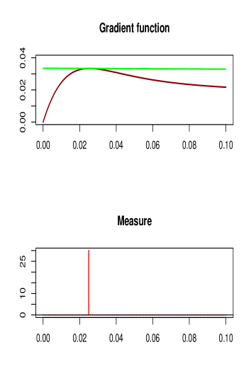
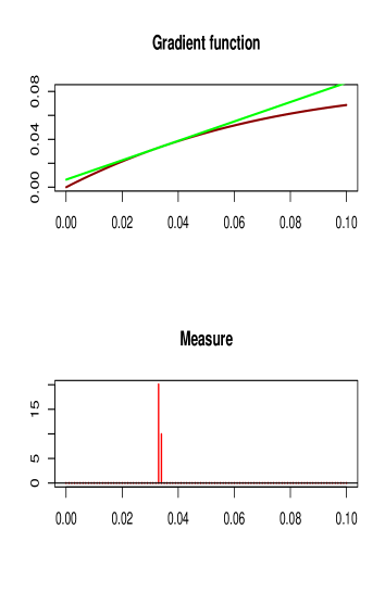
Numeric experiments conducted for various values of $u$ show that the obtained optimal solution is always one-atom as in the previous cases. Typically, the numeric solution gives two atoms at the neighbouring points of the discretised space $[0,1]$ for $x$ which indicates a single atom is situated in between these grid points, see Figure 3. Although we cannot formally prove that the optimum design is one-atom, such designs (i. e. equal doses) are certainly of an interest.

Figure 3: Numeric solution obtained by medea for $u=120$ (left pair of plots) and for $u=20$ (right pair) for $n=30$ mice. For $u=120$, the one-atom optimal measure is $30\,\delta_{x^{*}}$, where $x^{*}=0.02522$. The numeric solution is two-atomic: $29.97\,\delta_{0.025}+0.03\,\delta_{0.026}$. So, the total mass of $30$ was distributed between the grid points surrounding the true atom position. Similarly, for $u=20$ the one-atom optimal measure is $30\,\delta_{x^{*}}$ with $x^{*}=1/30$. The numeric solution is a two-atom measure $20.07\,\delta_{0.033}+9.93\,\delta_{0.034}$.

One-atom measures under constraint (8) have a form $\mu=n\delta_{x}$ for some $x\in(0,1/n]$. Making use of (26), we come to a one variable optimisation problem: maximise

$$G_{3}(n\delta_{x})=\log n-2\operatorname{{\bf E}}_{Q}\log\lambda+\operatorname{{\bf E}}_{Q}\log r(\lambda x)$$ (32)

subject to $x^{*}\leq 1/n$ and $Q$ is $\mathsf{Unif}[1,u]$. Only the last term depends on $x$, so the equivalent problem is to maximise

$$\tilde{G}_{3}(x;u)=\operatorname{{\bf E}}_{Q}\log r(\lambda x)=\frac{1}{u-1}\int_{1}^{u}\log r(\lambda x)\,d\lambda.$$

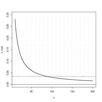
As $u$ grows, the maximum $x_{max}$ of this function, which can easily be computed numerically, approaches 0, see the right plot on Figure 4. So when $x_{max}\geq 1/n$, the constrained maximum is attained at the point $1/n$. Otherwise, for large $u$, $x_{max}<1/n$ and the solution is to take $n$ doses of volume $x_{max}$. This is exemplified at Figure 4 for $n=30$: the optimal dose is given by

$$x^{*}=\begin{cases}\frac{1}{n}&\quad u\leq u^{*};\\ x_{max}&\quad u>u^{*}.\end{cases}$$ (33)

where $u^{*}\approx 90.66$. This indicates that for those $u\leq u^{*}$ one needs to take all the substrate to make $n$ equal doses, and the volume $nx_{max}$ otherwise.

Figure 4: Left plot: function $\tilde{G}_{3}$ for $u=50,100$ and 200. As $u$ grows, the point of maximum $x_{max}$ approaches 0. The vertical dashed line is through the point $1/n$ with $n=30$. Right plot: $x_{max}$ as a function of $u$ (horizontal dashed line is through $1/n$ for $n=30$).

Finally, consider objective function $G_{4}$ given by (12) which corresponds to the expected asymptotic variance of the maximum likelihood estimator. In the case of a Uniform prior $\lambda\sim\mathsf{Unif}(1,u)$,

$$G_{4}(\mu;u)=-\frac{1}{u-1}\int_{1}^{u}I^{-1}(\mu;\lambda)\,d\lambda,$$ (34)

where $I(\mu;\lambda)$ is given by (31). Again, $G_{4}$ is Fréchet differentiable with the gradient function

$$g_{4}(x,\mu;u)=\frac{1}{u-1}\int_{1}^{u}I^{-2}(\mu;\lambda)\frac{e^{-\lambda x}}{1-e^{-\lambda x}}x^{2}\,d\lambda$$ (35)

and a numeric procedure should be used to find the optimal measure for any given values of $u$ and $n$. Similarly to the case of objective function $G_{3}$ above, numeric experiments show that the optimal measure is one atomic, although we cannot show this rigorously. In the class of one-atomic measures $\mu=n\delta_{x}$ the goal function simplifies to

$$G_{4}(n\delta_{x};u)=-\frac{e^{ux}-e^{x}-x(u-1)}{nx^{3}(u-1)}$$ (36)

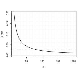
Similarly to $G_{3}$ above, the point of maximum $x_{max}$ of this function approaches 0 when $u$ grows, see the right plot on Figure 5. So that when $u$ is such that $x_{max}>1/n$ the optimal dose is $1/n$ (the whole substrate is used), otherwise the optimal dose is $x_{max}$. For example, for $n=30$ mice, the optimal dose is also given by (33) but with $u^{*}\approx 64.47$ this time.

Figure 5: Left plot: function $-\log(|nG_{4}(n\delta_{x};u)|)$ for $u=20,50$ and 100 (from upper to lower curve). As $u$ grows, the point of maximum $x_{max}$ approaches 0. The vertical dashed line is through the point $1/n$ with $n=30$. Right plot: $x_{max}$ as a function of $u$ (horizontal dashed line is through $1/n$ for $n=30$).

Gamma prior distribution.

Gamma prior distribution arises naturally as a posterior distribution for the Poisson parameter $\lambda$ which has a Uniform prior distribution. Since the probability of having $k$ pre-HSCs in the substrate is

$$\mathbf{P}\{\omega(V)=k\}=\operatorname{{\bf E}}_{Q}\mathbf{P}\{\omega(V)=k\mid\lambda\}=\frac{1}{u-1}\int_{1}^{u}\frac{\lambda^{k}e^{-\lambda}}{k!}\,d\lambda,$$ (37)

The posterior p.d.f. for $\lambda$ is then

$$f_{\lambda}(x\mid\omega(V)=k)=\frac{x^{k}e^{-x}}{\int_{1}^{u}\lambda^{k}e^{-\lambda}d\lambda}\propto x^{k}e^{-x},$$ (38)

which is close to $\Gamma(k+1,1)$ distribution for large $u$. So once an estimate for the total number of pre-HSCs k is available, the Gamma prior would be a reasonable for $\lambda$ in the subsequent experiment. Moreover, posterior distribution for a Gamma prior $\Gamma(\alpha,1)$ given $k$ pre-HSCs will be $\Gamma(\alpha+k,2)$ and so on. So generally, $\lambda\sim\Gamma(\alpha,\beta)$ with rate parameter $\beta\in\mathbb{N}$ could be a reasonable assumption.

Under this assumption, Criterion (10) becomes

$$G_{2}(\mu;\alpha,\beta)=\int_{0}^{\infty}\int_{(0,1]}f_{\alpha,\beta}(\lambda)\frac{e^{-\lambda x}}{1-e^{-\lambda x}}x^{2}\,\mu(dx)d\lambda\ ,$$ (39)

where

$$f_{\alpha,\beta}(\lambda)=\frac{\beta^{\alpha}}{\Gamma(\alpha)}\lambda^{\alpha-1}e^{-\beta\lambda}.$$ (40)

So $G_{2}$ is a linear functional with the gradient function

$$g_{2}(x,\mu;\alpha,\beta)=\int_{0}^{\infty}\frac{e^{-\lambda x}}{1-e^{-\lambda x}}x^{2}f_{\alpha,\beta}(\lambda)d\lambda=\int_{0}^{\infty}r(\lambda x)\lambda^{-2}f_{\alpha,\beta}(\lambda)d\lambda\\ =\frac{\beta^{2}}{(\alpha-1)(\alpha-2)}\int_{0}^{\infty}r(\lambda x)f_{\alpha-2,\beta}(\lambda)d\lambda\\ =\frac{\beta^{2}}{(\alpha-1)(\alpha-2)}\int_{0}^{\infty}r(\lambda)f_{\alpha-2,\beta/x}(\lambda)d\lambda.$$ (41)

Thus the situation here is similar to the case of the Uniform distribution: depending on whether the maximum of this function is below or above $1/n$ one needs to take equal doses of volumes $x_{max}$ the point where $g_{2}$ attains its maximum or $1/n$, respectively.

Consider as an example the first-iteration case when $\beta=1$. The gradient function and the point of maximum are shown in Figure 6. The optimal design is given by

$$x^{*}=\begin{cases}\frac{1}{n}&\quad\alpha\leq\alpha^{*};\\ x_{max}&\quad\alpha>\alpha^{*}.\end{cases}$$ (42)

where $\alpha^{*}\approx 49.68$.

Figure 6: Left plot: function $g_{2}(x)$ for $\beta=1$ and $\alpha=30,50,75,100$ (from top to bottom). The vertical dashed line is through the point $1/n$ with $n=30$. Right plot: $x_{max}$ as a function of $\alpha$ (horizontal dashed line is through $1/n$ for $n=30$ intersection the curve at point $u^{*}\approx 49.68$).

Under Gamma prior (40), criterion function (11) takes the following form:

$$G_{3}(\mu;\alpha,\beta)=\int_{0}^{\infty}f_{\alpha,\beta}(\lambda)\log I(\mu;\lambda)d\lambda,$$ (43)

where $I(\mu;\lambda)$ is given by (31). Note that $G_{3}$ is not a linear functional of a measure, however it is Fréchet differentiable with the gradient function

$$g_{3}(x,\mu;\alpha,\beta)=\int_{0}^{\infty}I^{-1}(\mu;\lambda)\frac{e^{-\lambda x}}{1-e^{-\lambda x}}x^{2}f_{\alpha,\beta}(\lambda)d\lambda.$$ (44)

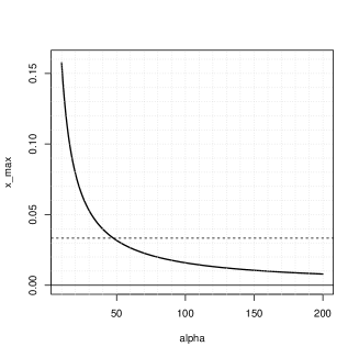
Thus, as before numeric methods for $\beta=1$ and a given values of $\alpha$ and $n$ should be employed. Our experiments show that the optimum measure given by the steepest descent algorithm still contains only one atom. So, optimising (43) for one atomic measures $n\delta_{x}$ over $x\in(0,1/n]$ leads to the design given by (42), with $\alpha^{*}\approx 47.70$. Figure 7 shows $G_{3}(n\delta_{x};\alpha)$ and the optimal equal doses for different values of $\alpha$.

Figure 7: Left plot: function ${G}_{3}(n\delta_{x};\alpha)$ for $\beta=1$ and $\alpha=50,100$ and 200. Similarly to the Uniform prior case as $\alpha$ grows, the point of maximum $x_{max}$ approaches 0. The vertical dashed line is through the point $1/n$ with $n=30$. Right plot: $x_{max}$ as a function of $\alpha$ (horizontal dashed line is through $1/n$ for $n=30$).

Finally, consider $G4$ in (12) with Gamma prior distribution on $\lambda$:

$$G_{4}(\mu;\alpha,\beta)=-\int_{0}^{\infty}I^{-1}(\mu;\lambda)f_{\alpha,\beta}(\lambda)d\lambda,$$ (45)

which is Fréchet differentiable with the gradient function

$$g_{4}(x,\mu;\alpha,\beta)=\int_{0}^{\infty}I^{-2}(\mu;\lambda)\frac{e^{-\lambda x}}{1-e^{-\lambda x}}x^{2}f_{\alpha,\beta}(\lambda)d\lambda.$$ (46)

Here also, our numeric experiments for $\beta=1$ and any given values of $\alpha$ and $n$, show that the optimal measure contains a single atom. Thus, in the class of one atomic measures, (45) simplifies to

$$G_{4}(n\delta_{x};\alpha)=-\dfrac{1}{nx^{2}}\int_{0}^{\infty}\frac{1-e^{-\lambda x}}{e^{-\lambda x}}f_{\alpha}(\lambda)d\lambda.$$ (47)

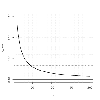
which leads to the one-atom optimal design (42) with $\alpha^{*}\approx 45.74$, see Figure 8.

Figure 8: Left plot: function $-\log(|nG_{4}(n\delta_{x};\alpha)|)$ for $\beta=1$ and $\alpha=20,50$ and 100. Similar to the Uniform case for $G_{4}$, as $\alpha$ grows, the point of maximum $x_{max}$ approaches 0. The vertical dashed line is through the point $1/n$ with $n=30$. Right plot: $x_{max}$ as a function of $\alpha$ (horizontal dashed line is through $1/n$ for $n=30$).

4.3 Optimal design with additional costs

The measure optimisation formalism we used above allows for seamless inclusion of different costs associated with the experiment either as additional terms in the goal function or as additional contraints. This can be done in both non-Bayesian and Bayesian settings. Typical loss incured in the above described experiment are the non-repopulated laboratory mice which are quite expensive. Added to this, the cost of all the experiment when all mice die or all mice survive so if it does not yield meaningful results. In this section we demonstrate how these costs affect the optimal experimental design.

Non-Bayesian setting.

To take into account the cost of non-repopulated mice, note that for a fixed $\lambda$, the indicator $\chi_{i}$ that the mouse which received the $i$th dose of volume $x_{i}$ has not repopulated is a Bernoulli random variable with a parameter $e^{-\lambda x_{i}}$, see (3). Thus, the mean number of non-repopulated mice $\operatorname{{\bf E}}\sum_{i=1}^{n}\chi_{i}$ is

$$T_{1}(\mathbf{x};\lambda)=\sum_{i=1}^{n}e^{-\lambda x_{i}},$$ (48)

which can be represented as a functional of the design measure $\mu$ as follows:

$$T_{1}(\mu;\lambda)=\int e^{-\lambda x}\mu(dx).$$ (49)

Recall that as in the previous sections, all the integrals are taken over the range $(0,1]$. To include the cost associated with a spoilt experiment, compute the probability that all the mice do not repopulate which can be written as follows:

$$T_{21}(\mathbf{x};\lambda)=\prod_{i}^{n}\mathbf{P}\{\chi_{i}=1\}$$

$$=\prod_{i=1}^{n}e^{-\lambda x_{i}}=e^{-\lambda\sum_{i=1}^{n}x_{i}}.$$ (50)

Consequently, the probability that all the mice repopulate is

$$T_{20}(\mathbf{x};\lambda)=\prod_{i=1}^{n}\mathbf{P}\{\chi_{i}=0\}=\prod_{i=1}^{n}(1-e^{-\lambda x_{i}})=e^{\sum_{i=1}^{n}\log(1-e^{-\lambda x_{i}})}.$$ (51)

In terms of the design measure, (4.3) and (51) are the following functionals:

$$T_{21}(\mu;\lambda) =e^{-\lambda\int x\mu(dx)}$$ (52)

$$T_{20}(\mu;\lambda) =e^{\int\log(1-e^{-\lambda x})\mu(dx)}.$$ (53)

This gives rise to the expression for the probability of a spoilt experiment due to either all the mice repopulating or all the mice non-repopulating:

$$T_{2}(\mu;\lambda)=T_{21}(\mu;\lambda)+T_{20}(\mu;\lambda).$$ (54)

We note that $T_{1}$ and $T_{2}$ are Fréchet differentiable with the gradient functions

$$t_{1}(x;\lambda)=e^{-\lambda x}$$ (55)

and

$$t_{2}(x,\mu;\lambda)=-\lambda x\,T_{21}(\mu;\lambda)+\log(1-e^{-\lambda x})\,T_{20}(\mu;\lambda).$$ (56)

Now consider maximisation of a new goal function

$$\tilde{G_{1}}(\mu;\lambda)=G_{1}(\mu;\lambda)-c_{1}T_{1}(\mu;\lambda)-c_{2}T_{2}(\mu;\lambda),$$ (57)

where $G_{1}$ is given by (7), under constraints (8) and (9). The positive constants $c_{1},c_{2}$ should be set by the experimentator to reflect the cost of mice and of a spoilt experiment which should be offset against the usefulness of the results reflected in the original goal function $G_{1}$ involving the Fisher information.

The function $\tilde{G_{1}}$ is strongly diferentiable with the gradient function given by

$$\tilde{g_{1}}(x,\mu;\lambda)=g_{1}(x;\lambda)-c_{1}t_{1}(x;\lambda)-c_{2}t_{2}(x,\mu;\lambda),$$ (58)

where $g_{1}$ as in (25).

Figure 9 shows the optimal dose as a function of $\lambda$, for $n=30$, $c_{1}=10^{-4}$ and $c_{2}=1$. Compared to the optimal design for $G_{1}$ shown on Figure 1 one has to dilute more and also to start dilution earlier at $\lambda=41.8$ compared to 47.8 for $G_{1}$ which reflects the caution not to allow all the mice to survive as this would mean a spoilt experiment.

Figure 9: The optimal doses for different values of $\lambda$ for the goal function $\tilde{G_{1}}$ when $n=30$, $c_{1}=10^{-4}$ and $c_{2}=1$ (dashed) and for $G_{1}$ (solid line) as on Plot (c) in Figure 1.

Bayesian setting.

Under $\Gamma(\alpha,1)$ prior distribution for $\lambda$, the average number of non-repopulated mice becomes

$$\operatorname{{\bf E}}_{Q}T_{1}(\mu;\lambda)=\int\frac{1}{(1+x)^{\alpha}}\mu(dx),$$ (59)

with the gradient function

$$\operatorname{{\bf E}}_{Q}t_{1}(x;\lambda)=\frac{1}{(1+x)^{\alpha}}.$$ (60)

The probability of a spoilt experiment is

$$\operatorname{{\bf E}}_{Q}T_{2}(\mu;\lambda) =\operatorname{{\bf E}}_{Q}T_{21}(\mu;\lambda)+\operatorname{{\bf E}}_{Q}T_{20}(\mu;\lambda)$$ (61)

$$=\dfrac{1}{(1+H(\mu))^{\alpha}}+\operatorname{{\bf E}}_{Q}T_{20}(\mu;\lambda),$$ (62)

with the corresponding gradient function

$$\operatorname{{\bf E}}_{Q}t_{2}(x,\mu;\lambda)=-\dfrac{\alpha x}{(1+H(\mu))^{\alpha+1}}+\operatorname{{\bf E}}_{Q}\log(1-e^{-\lambda x})T_{20}(\mu;\lambda),$$ (63)

where $H(\mu)=\int x\mu(dx)$.

Take $G_{4}$ as in (45) with $\beta=1$ and consider a new goal function

$$\tilde{G_{4}}(\mu;\alpha)=G_{4}(\mu;\alpha)-c_{1}\operatorname{{\bf E}}_{Q}T_{1}(\mu;\lambda)-c_{2}\,\operatorname{{\bf E}}_{Q}T_{2}(\mu;\lambda).$$ (64)

It is Fréchet differentiable and possesses a gradient function

$$\tilde{g_{4}}(x,\mu;\alpha)=g_{4}(\mu,x;\alpha)-c_{1}\operatorname{{\bf E}}_{Q}t_{1}(x;\lambda)-c_{2}\operatorname{{\bf E}}_{Q}t_{2}(x,\mu;\lambda).$$ (65)

We are aiming to maximise $\tilde{G_{4}}$ under the same constraints (8) and (9).

Again, numeric solutions are still one-atomic for different tried values of the parameters $\alpha,c_{1}$ and $c_{2}$ we tried. Figure 10 shows a typical picture for $-\log|\tilde{G_{4}}(n\delta_{x};\alpha)|$ for the class of one-atomic design measures and the optimal doses for three different values of $\alpha$.

Figure 10: Function $-\log|\tilde{G_{4}}(n\delta_{x};\alpha)|$ for the costs $c_{1}=0.005$, $c_{2}=5$ and values $\alpha=30,50,100$ (in the order of a decrease). The vertical dashed line is through the point $1/n$ with $n=30$. The extremal points are $x_{max}=0.043,0.028$ and $0.015$ leading to optimal designs $1/30,0.028$ and $0.015$, respectively.

Mixture prior distribution

Finally, consider the setting typical for testing two alternative hypotheses about possible values of the mean number of pre-HSCs. Suppose that $\lambda$ can take two different values, our prior belief is that it is rather $\lambda_{1}$ than $\lambda_{2}$ with probability $0<p<1$. This gives rise to optimisation of the following goal function

$$G_{1M}(\mu;p,\lambda_{1},\lambda_{2})=p\ G_{1}(\mu;\lambda_{1})+(1-p)\ G_{1}(\mu;\lambda_{2}).$$ (66)

under constraints (8) and (9).

The gradient function for (66) is

$$g_{1M}(x;p,\lambda_{1},\lambda_{2})=p\ g_{1}(x;\lambda_{1})+(1-p)\ g_{1}(x;\lambda_{2}).$$ (67)

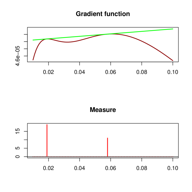
and numerical optimisation can be employed to find the optimal design for any particular values of $\lambda_{1},\lambda_{2}$ and $p$. For example of $\lambda_{1}=25,\lambda_{2}=150$ and $p=0.05$, Figure 11 shows a numerically obtained optimal measure which is two-atomic: 19 mice should receive equal doses of $0.019$ and the rest 11 of them should receive the same doses of $0.058$.

Figure 11: Solution obtained by medea for $p=0.05$, $\lambda_{1}=25$, and $\lambda_{2}=150$ shows that the numeric solution is a two atomic measure $18.98\ \delta_{0.019}+11.02\ \delta_{0.058}$ and all the substrate should be used.

5 Discussion

We have considered dilution experiments with volume constraints typical in biological and medical research. An important particularity of the experiments we consider here is that the time delay necessary for pre-HSCs to develop and then for the injected doses to take effect in mice prevents from planing multiple stage experiments: the estimation should necessarily be done from the first and only stage. As we have seen, in all the considered cases of the goal functions, the optimal design is attained on a one-point measure, meaning that all the doses should have equal volume. This parallels the well known result about the D-optimal design measure for a linear regression model: The Kiefer-Wolfowitz theorem assures that such measure is atomic with the number of atoms to be at most the number of contraints plus one, see, e. g., Kiefer:1960. In our case we have one volume constraint (in addition to the measure to have a fixed total mass) so the number of atoms is at most two. Indeed, the gradient functions we observed are convex on the interval from 0 to the point of maximum, so the only possibility to satisfy the necessary optimality condition given in Theorem 2, is for the optimal measure to have only one atom. However, the example of a mixture prior distribution considered in the last section shows that two-atom designs are indeed possible.

In practical terms, if the number of pre-HSC expected to be not very large (a few dozens or less), the whole substrate should be used to derive the doses, otherwise only part of it. We have characterised above what is ‘not very large’ and how much the doses should be diluted. We have fixed some of the parameters here (the number of mice $n=30$, $\beta=1$), driven by practical applications to stem cell research. For other applications and other values of these parameters one make use the computer codes the authors make freely available for download.

Advantage of measure optimisation approach is that additional requirements can be easily incorporated into the goal function or added as further constraints, e. g. limited cost associated with non-repopulated mice and/or the cost of the whole experiment if all mice are repopulated or all are not repopulated.

References

- [\citeauthoryearAtkinson and DonevAtkinson and Donev1992] Atkinson, A. C. and A. N. Donev (1992). Optimum Experimental Designs. Oxford: Clarendon Press.
- [\citeauthoryearBonnefoix and CallananBonnefoix and Callanan2010] Bonnefoix, T. and M. Callanan (2010). Accurate hematopoietic stem cell frequency estimates by fitting multicell poisson models substituing to the single-hit poisson model in limiting dilution transplantation assays. Blood 116(14), 2472–2475.
- [\citeauthoryearChaloner and LarntzChaloner and Larntz1989] Chaloner, K. and K. Larntz (1989). Optimal bayesian design applied to logistic regression experiments. J. Statis. Planng Inf. 21, 191–208.
- [\citeauthoryearCochranCochran1950] Cochran, W. G. (1950). Estimation of bacterial densities by means of the ”Most Probable Number”. Biometrics 6, 105–116.
- [\citeauthoryearCominettiCominetti1990] Cominetti, R. (1990). Metric regularity, tangent sets, and second-order optimality conditions. Appl. Math. Optim. 21, 265–287.
- [\citeauthoryearDaley and Vere-JonesDaley and Vere-Jones2008] Daley, D. J. and D. Vere-Jones (2008). An Introduction to the Theory of Point Processes. Volume II: General Theory and Structure (2nd ed.). New York: Springer.
- [\citeauthoryearDunford and SchwartzDunford and Schwartz2009] Dunford, N. and J. T. Schwartz (2009). Linear Operators: Part 1, General Theory. New Jersey: John Wiley & Sons.
- [\citeauthoryearEveritt and SkrondalEveritt and Skrondal2010] Everitt, B. S. and A. Skrondal (2010). The Cambridge dictionary of statistics, 4th edition. New York: Cambridge university press.
- [\citeauthoryearFisherFisher1922] Fisher, R. A. (1922). On the mathemtical foundation of theoretical statistics. Philosophical Transactions of the Royal Society of London. Series A, Containing Papers of a Mathematical or Physical Character. 222, 309––368.
- [\citeauthoryearGekas, Dieterlen-Lievre, Orkin, and MikkolaGekas et al.2005] Gekas, C., F. Dieterlen-Lievre, S. H. Orkin, and H. K. A. Mikkola (2005). The placenta is a niche for hematopoietic stem cells. Developmental 8, 365–375.
- [\citeauthoryearHallHall1988] Hall, P. (1988). Introduction to the theory of Coverage Processes. New York: Wiley.
- [\citeauthoryearHille and PhilipHille and Philip1957] Hille, E. and R. S. Philip (1957). Functional Analysis and Semigroups. New York: American Mathematical Society.
- [\citeauthoryearKiefer and WolfowitzKiefer and Wolfowitz1960] Kiefer, J. and J. Wolfowitz (1960). The equivalence of two extremum problems. Canadian Journal of Mathematics. 12, 363–366.
- [\citeauthoryearKumaravelu, Hook, Morrison, Ure, Zhao, Zuyev, Ansell, and MedvinskyKumaravelu et al.2002] Kumaravelu, R., L. Hook, A. M. Morrison, J. Ure, S. Zhao, S. Zuyev, J. Ansell, and A. Medvinsky (2002). Quantitative developmental anatomy of definitive haematopoietic stem cells/long-term repopulating units (hsc/rus): role of the aorta-gonad-mesonephros (agm) region and the yolk sac in colonisation of the mouse embryonic liver. Developmental 129, 4891–4899.
- [\citeauthoryearMarin and RobertMarin and Robert2007] Marin, J. and C. P. Robert (2007). Bayesian Core: A Practical Approach to Computational Bayesian Statistics. New York: Springer.
- [\citeauthoryearMaurer and ZoweMaurer and Zowe1979] Maurer, H. and J. Zowe (1979). First and second order necessary and sufficient optimality conditions for infinite-dimensional programming problems. Math. Programming 16, 98–110.
- [\citeauthoryearMayhall, Paffett-Lugassy, and ZonMayhall et al.2004] Mayhall, E. A., N. Paffett-Lugassy, and L. I. Zon (2004). The clinical potential of stem cells. Current Opinion in Cell Biology. 16(6), 713––720.
- [\citeauthoryearMcCradyMcCrady1915] McCrady, M. H. (1915). The numerical interpretation of fermentation-tube results. The Journal of Infectious Diseases 17(1), 183–212.
- [\citeauthoryearMedvinsky, Rybtsov, and TaoudiMedvinsky et al.2011] Medvinsky, A., S. Rybtsov, and S. Taoudi (2011). Embryonic origin of the adult hematopoietic system: advances and questions. Development. 138, 1017–1031.
- [\citeauthoryearMolchanov and ZuyevMolchanov and Zuyev2000a] Molchanov, I. and S. Zuyev (2000a). Tangent sets in the space of measures: with applications to variational calculus. J. Math. Anal. Appl. 249, 539–552.
- [\citeauthoryearMolchanov and ZuyevMolchanov and Zuyev2000b] Molchanov, I. and S. Zuyev (2000b). Variational analysis of functionals of a poisson process. Math. Oper. Res. 25, 485–508.
- [\citeauthoryearMolchanov and ZuyevMolchanov and Zuyev2002] Molchanov, I. and S. Zuyev (2002). Steepest decent algorithm in a space of measures. Statistics and Computing 12(2), 115–123.
- [\citeauthoryearMolchanov and ZuyevMolchanov and Zuyev2004] Molchanov, I. and S. Zuyev (2004). Optimization in space of measures and optimal design. ESAIM 8, 12–24.
- [\citeauthoryearOttersbach and DzierzakOttersbach and Dzierzak2005] Ottersbach, K. and E. Dzierzak (2005). The murine placenta contains hematopoietic stem cells within the vascular labyrinth region. Dev. Cell. 8, 377–387.
- [\citeauthoryearPukelsheimPukelsheim1983] Pukelsheim, F. (1983). Optimal Design of Experiments. New York: Wiley.
- [\citeauthoryearRidoutRidout1995] Ridout, M. S. (1995). Three-stage design for seed testing experiments. Appl. Statist. 44, 153–162.
- [\citeauthoryearRobinsonRobinson1976] Robinson, S. M. (1976). First order conditions for general nonlinear optimization. SIAM J. Appl. Math. 30, 597–607.
- [\citeauthoryearSchneiderSchneider1988] Schneider, R. (1988). Random approximations of convex sets. J. Microscopy 151, 211–227.
- [\citeauthoryearWynn and ZhigljavskyWynn and Zhigljavsky1994] Wynn, H. P. and A. A. Zhigljavsky (1994). The theory of search from a statistical viewpoint. Test 3, 1–45.
- [\citeauthoryearZacksZacks1977] Zacks, S. (1977). Problems and approaches in design of experiments for estimation and testing in non-linear models. In Multivariate Analysis 4, 209–223.
- [\citeauthoryearZhigljavskyZhigljavsky1991] Zhigljavsky, A. A. (1991). Theory of Global Random Search. Dordrecht: Kluwer Academic.
- [\citeauthoryearZowe and KurcyuszZowe and Kurcyusz1979] Zowe, J. and S. Kurcyusz (1979). Regularity and stability for the mathematical programming problem in banach spaces. Appl. Math. Optim. 5, 49–62.