Consequence of total lepton number violation in strongly magnetized iron white dwarfs

Abstract

The influence of a neutrinoless electron to positron conversion on a cooling of strongly magnetized iron white dwarfs is studied. It is shown that they can be good candidates for soft gamma-ray repeaters and anomalous X-ray pulsars.

I Introduction

The white dwarfs (WDs) are quite numerous in the Milky Way YT and the astrophysics of these compact objects is nowadays a well developed domain KC ; BH ; ACIG . Since the interior of the WDs is considered to be fully degenerate, studying their properties provides a fundamental test of the concept of stellar degeneracy. The important observables, which could test models of structure and evolution of WDs, are the luminosity and the effective (surface) temperature.

Steady progress in understanding of the WDs cooling processes and precise measurements of their luminosity curve and of their effective temperature open a door to their possible use as a laboratory for analyzing some problems of elementary particles physics. Thus, Isern et al. IEA1 ; IEA2 suggested studying possible existence of axions on a basis of the WDs luminosity function. Following this idea, we analyze the influence of the lepton number violation on the luminosity and the effective temperature of strongly magnetized iron WDs (SMIWDs). As it is well known, the existence of the Majorana type neutrino would imply the lepton number violating process of electron capture by a nucleus X($A,Z$)

$$\mathrm{e}^{-}+\mathrm{X}(A,Z)\rightarrow\mathrm{X}(A,Z-2)+\mathrm{e}^{+}\ .$$ (1)

This reaction is an analogue of the neutrinoless double beta-decay, intensively studied these days VES . Very recent experimental results on this process, obtained with the ⁷⁶Ge detectors, can be found in Refs. GD ; MAJ . An estimate MAJ shows that to attain for the neutrino masses sensitivities in the region of 15 - 50 meV, tonne-scale detectors are needed. At present the detectors GD ; MAJ comprise tens of kilograms of ⁷⁶Ge. Since 1 kg of ⁷⁶Ge includes 8.31 $\times$ 10²⁴ atoms, a tonne device would contain $\sim$ 10²⁸ of ⁷⁶Ge atoms. On the other hand, the matter density of the SMIWDs is at the level of 10³³/cm³ and more, which is by several orders of magnitude larger. This fact makes the study of reaction (1) in stellar medium attractive.

For the weak reaction (1) with the rate proportional to the square of a small neutrino mass to be detectable, it has to take place in a bulk of the stellar body with a well understood background. It is allowed energetically when the Fermi energy $E_{\,\mathrm{F}}$ of the electron gas is larger than the threshold energy $\Delta^{\beta\beta}_{Z}$ given by the mass difference between the final and the initial nuclei plus the electron mass. However, as it can be seen from Table 1, in the WDs consisting of the even-even nuclei the threshold energy of the inverse beta decay $\Delta^{\beta}_{Z}$ is smaller than $\Delta^{\beta\beta}_{Z}$ + $m_{\mathrm{e}}c^{2}$ ($m_{\mathrm{e}}$ is the electron mass and $c$ is the light velocity). Since usually $\Delta^{\beta}_{Z-1}\,<\,\Delta^{\beta}_{Z}$, two successive decays EES ; ST ; RRRX ; BK1 ; BS

$$(A,Z)\,\rightarrow\,(A,Z-1)\,\rightarrow\,(A,Z-2)\,$$ (2)

proceed, unless all $(A,Z)$ nuclei transform to $(A,Z-2)$ nuclei, and the reaction (1) cannot occur. The point is that in the WDs, the electron Fermi energy $E_{\,\mathrm{F}}$ cannot overcome the energy at which the inverse beta decay proceeds. For the case of the ${}^{56}_{26}$Fe nuclei, this situation is discussed in detail in Ch. 3 of Ref. ST . Instead of compression increasing $E_{\,\mathrm{F}}$ and, therefore, the pressure, the electrons are captured by the iron nuclei which are transformed in the two-step process (2) into the chrome ones. So the onset of the inverse beta decay at the density $\rho_{B}$=(1.14 - 1.18) $\times$ 10⁹ g/cm³ terminates the iron WD ST ; RRRX . As can be seen from the Table III of Ref. RRRX , this density is also critical one for the onset of the instability due to the general relativity and the subsequent collapse of the ${}^{56}_{24}$Cr WD happens. So, the only chance to have the reaction (1) in the bulk of compact objects are the SMWDs, where it can hold $E_{\,\mathrm{F}}$ $>$ $\Delta^{\beta\beta}_{Z}$ + $m_{\mathrm{e}}c^{2}$ due to the presence of the strong magnetic field.

Besides our choice for X($A,Z$) = ${}^{56}_{26}$Fe(0,0⁺) and for X($A,Z-2$) = ${}^{56}_{24}$Cr(0,0⁺) in the process (1), other pairs of the even-even nuclei in the ground state (0,0⁺) can be taken. They are given in Table 1, together with the value of the threshold energies $\Delta^{\beta\beta}_{Z}$ and $\Delta^{\beta}_{Z}$. Since the energy $E_{e}$ of electrons that can participate in the reaction (1) should satisfy inequality

$$m_{\mathrm{e}}c^{2}+\Delta^{\beta\beta}_{Z}<E_{\mathrm{e}}<E_{\,\mathrm{F}}\,,$$ (3)

it follows from Table 1 that there are more active electrons for the nuclei with smaller values of $\Delta^{\beta\beta}_{Z}$. On the other hand, the inverse beta decay process cannot occur in the nucleus ${}^{12}_{\,\,\,6}$C in reality. This follows from comparing the critical densities for the onset of the inverse beta decay $\rho^{\beta,\mathrm{relFMT}}_{\mathrm{crit}}$ and for the gravitational instability $\rho^{\mathrm{FMTrel}}_{\mathrm{crit}}$ , as given in Table II and Table III RRRX , respectively,

$$\rho^{\beta,\mathrm{relFMT}}_{\mathrm{crit}}=3.97\,\times\,10^{10}\,\mathrm{g/cm^{3}}\,,\,\,\,\rho^{\mathrm{FMTrel}}_{\mathrm{crit}}=2.12\,\times\,10^{10}\,\mathrm{g/cm^{3}}\,.$$ (4)

It also follows from the inequality (3) and from Table 1 that the reaction (1) would be strongly suppressed in the ${}^{16}_{\,\,\,8}$O SMWDs in comparison with the case of SMWDs composed of heavier nuclei.

Let us also note that our choice of the SMIWDs was influenced by the existence of extensive calculations of the properties of the iron WDs for the matter densities small enough to avoid the inverse beta decay PAB and also for the case when the inverse beta decay takes place BK1 ; BS ; BK2 . This will allow us to make a qualitative comparison of our results with these already existing ones.

The non-magnetized iron-core WDs were first studied in Ref. SHV . A comprehensive study of the properties of iron-core WDs with emphasis placed on their evolution was performed in Ref. PAB . In particular, the crystallization, electrostatic corrections to the equation of state, conductive opacity and neutrino emission were taken into account. The work PAB was inspired by new observational data provided by the satellite Hypparcos, from which the existence of three iron-core WDs (GD 140, EG 50 and Procyon B) was suggested PROV1 ; HLSJLP . For Procyon B, being situated close to Procyon A, one of the brightest stars in the sky, it was difficult to obtain good data and later on, it was put ’outside the iron box’ and classified as a rare DQZ WD PROV2 . For EG 50 and GD 140 the results were robust enough for Provencal et al. to conclude that the only way how to explain the observations was to assume an iron, or an iron-rich, core composition of these two WDs. Only then it was possible to fit the observed radii, masses, and surface gravities consistently. This opened the problem of understanding formation of these WDs, because such a core composition is at variance with current theories.

Later on, Fontaine et al. FBB reconsidered the problem with the EG 50 core composition by improving the accuracy of the effective temperature $T_{\mathrm{eff}}$ and surface gravity $g$ of the EG 50 deduced from optical spectroscopy. Since these values turned out to be entirely consistent with those used in Ref. PROV1 , they concluded that the problem with the iron-core of EG 50 does not lie in inaccuracy of spectroscopic data. Subsequent calculations FBB of the distance with various core compositions and its comparison with the observed distances $d=15.41\begin{array}[]{c}+0.84\\ -0.71\end{array}$ pc, provided by Hypparcos PROV1 , and $d=15.08\begin{array}[]{c}{+0.50}\\ {-0.40}\end{array}$ pc from the Yale Parallax Program, show (see Fig. 2 FBB ) that cores made of C, O, Ne, Mg, Si, S and Ca are excluded and only models with heavier element cores Ar, Ti, Cr, Fe provide acceptable solutions. Then Fontaine et al. conclude that the case of EG 50 shows that the WD formation process is not fully understood.

It can be concluded from the discussed material that the main source of uncertainty of the core composition of EG 50 is in the parallax. It is expected that the uncertainty will diminish essentially with the new precise data from GAIA MABEAL .

It also follows that our choice of the SMIWDs is well founded, because calculations comparable with Refs.  PAB ; BK1 ; BS ; BK2 for other possible elements do not exist.

Nowadays, two possible physical processes able to account for the formation of iron core WDs are available ICL ; OSJ . In Ref. OSJ , namely the case of the WD EG 50 is considered and a simple model for the explanation of its Fe-rich composition is proposed. If a low-mass X-ray binary, consisting of a neutron star and a WD, is sufficiently tight, under certain assumptions, ejecta from the exploding neutron star trigger nuclear burning in the WD, possibly leading to the WD with Fe-rich composition with the mass $0.43M_{\odot}<M_{\mathrm{WD}}<0.72M_{\odot}$, reminiscent of EG 50.

Rather exotic solution of the above discussed problem has been proposed in Ref. MEAL , considering possibility that such more compact WDs as ED 50 or GD 140 are (characterized by falling away from the expected C/O relationship in the M-R diagram), could have in the core a portion of strange matter gained after accreting a strange-matter nugget. Such nuggets could exist (see Ref. MEAL and the references therein) either as a relic of the early universe or as an ejected fragment from the merger/coalescence of strange-matter neutron stars. However, as is well known ST ; PPNS , the strange matter could be present only in the inner core of rather massive NSs with the mass $M\gtrsim$ 1.4 - 1.5 $M_{\odot}$, where the matter density $\rho\,\gtrsim 2\,\rho_{0}$. So it is not clear how could be the strange matter maintained in the core of WDs that have the central density smaller by several orders in the magnitude.

Let us also present the study CRIG in which a common proper motion pair formed by a WD0433+270 and a main-sequence star BD+26730 is studied with aim to investigate whether this system belongs to the Hyades cluster. In the affirmative case, the calculations of cooling sequence for different core compositions based on the results of PAB show that the WD member of the pair could have an iron core. The kinematic and chemical composition considerations provided enough material for Catalan et al. to make believe that the pair was a former member of the Hyades cluster and consequently, it has an evolutionary link to it. However, the evidence is not yet fully conclusive.

Table 1: The pairs of the even-even nuclei with which the reaction (1) can proceed, for which $\Delta^{\beta\beta}_{Z}$ are the threshold energies, calculated using the atomic mass evaluation AWT ; $\Delta^{\beta}_{Z}$ are the threshold energies of the inverse beta decay. Their values were taken from Refs. BK1 ; BS . In the 5th, 8th and 9th rows, they contain also the excitation energies of the 1⁺ level of the related $(A,Z-1)$ nuclei, because the transitions to the ground level are strongly suppressed.

X($A,Z$)	X($A,Z-2$)	$\Delta^{\beta\beta}_{Z}$ [MeV]	$\Delta^{\beta}_{Z}$ [MeV]
${}^{12}_{\,\,\,6}$C	${}^{12}_{\,\,\,4}$Be	27.0	13.370
${}^{16}_{\,\,\,8}$O	${}^{16}_{\,\,\,6}$C	19.45	10.419
${}^{32}_{16}$S	${}^{32}_{14}$Si	2.96	1.708
${}^{56}_{26}$Fe	${}^{56}_{24}$Cr	6.33	3.794
${}^{42}_{20}$Ca	${}^{42}_{18}$Ar	5.15	3.524
${}^{60}_{28}$Ni	${}^{60}_{26}$Fe	4.08	2.890
${}^{66}_{30}$Zn	${}^{66}_{28}$Ni	3.92	2.630
${}^{72}_{32}$Ge	${}^{72}_{30}$Zn	5.48	4.260

While considering the process (1) in SMIWDs is theoretically tempting, it should be pointed out that their astrophysical studies have only started to develop. In particular, microscopic models of their development, of their internal structure or of their cooling process have not yet been developed to a point of general acceptance and to convincing tests by astrophysical data, though the very recent publications BEBH ; DM6 have made a basic breakthrough in the understanding the structure of the SMWDs. In several next paragraphs, we give a brief survey of recent developments.

Detailed study of a strongly magnetized cold electron gas and its application to the SMWDs has recently been done in Refs. KM ; DM ; DM1 ; DM2 . This theory stems from the Landau quantization of the motion of electrons in a magnetic field LL ; SDM and of its modification to the case of a very strong magnetic field LS with a strength ${\cal B}\geq{\cal B}_{c}$. It turns out that in systems with small number of Landau levels, which is restricted by a suitable choice of the strength of the magnetic field and of the maximum of the Fermi energy $E_{\,\mathrm{F}}$ of the electron gas, the mass of the SMWD can be in the range (2.3 - 2.6) $M_{\odot}$. It means that the strong magnetic field can enhance the energy of the electron gas to such a level that its pressure will force the gravity to allow the SMWD to have a mass larger than the Chandrasekhar-Landau (CL) limit of 1.44 $M_{\odot}$ C ; L .

The existence of the WDs with the mass exceeding the CL limit has recently been deduced from the study of the observed light curves for highly luminous type Ia supernovae. For instance, it was found in the case of the SN 2009dc KEAL that such a model WD – a progenitor of the supernova – can be formed, if a mass accretion is combined with a rapid rotation. The comparison of calculations and the observations yielded an estimate of the WD mass within the limit of (2.2 - 2.8) $M_{\odot}$. The problem is that although the rotating WD is supposed to resist the gravitational collapse up to the mass $\approx$ 2.7 $M_{\odot}$ HEAL , no convincing calculations of such a WD mass limit exist so far in this model. The maximum stable mass of general relativistic uniformly rotating WDs, computed in Ref. BRR within the Chandrasekhar approximation for the equation of state, is $M_{\,\mathrm{max}}$ = 1.51595 $M_{\odot}$ for the average nuclear composition $\mu$ = 2. Later calculations BRRS , with the WD matter described by the relativistic Feynman-Metropolis-Teller equation of state, provided $M_{\,\mathrm{max}}$ = 1.500, 1.474, 1.467, 1.202 $M_{\odot}$ for ⁴He, ¹²C, ¹⁶O, and ⁵⁶Fe, respectively.

On the other hand, according to Refs. DM3 ; DMR , a new mass limit $\approx$ 2.6 $M_{\odot}$ can be derived KM ; DM ; DM1 in a model describing the SMWDs as a system of the relativistic degenerate electron gas in the strong magnetic field, in which the SMWD with the mass $\approx$ 2.6 $M_{\odot}$ lies at the end of a mass-radius curve for the one Landau level system, corresponding to the central magnetic field 8.8 $\times$ 10¹⁷ G, when the Fermi energy $\epsilon_{\,\mathrm{F}}$ in units of the electron mass is $\epsilon_{\,\mathrm{F}}$=$E_{\,\mathrm{F}}/m_{\mathrm{e}}\,c^{2}$= 200. To achieve such a mass, it was supposed that the continuously accreting WD is being compressed by the gravity, which steadily increases the strength of the magnetic field, because the total magnetic flux is conserved. At the end, the magnetic field in the core can exceed the critical value ${\cal B}_{c}$, the WD becomes the SMWD, and the pressure of the relativistic degenerate electron gas is able to balance the gravity up to the point, when the accreting mass raises the SMWD mass up to $\approx$ 2.6 $M_{\odot}$, after which the SMWD collapses and the supernova of the type Ia explodes .

Let us note that the concept of the SMWDs developed in Refs. KM ; DM ; DM1 ; DM3 ; DMR has been recently criticized by several authors NK ; CFD ; CMFP ; CEAL . The response to this criticism can be found in Refs. DM2 ; DM5 .

It should be pointed out that neither side of this dispute can support its point of view by consistent detailed calculations, which should take into account violation of spherical symmetry and effects of general relativity: rather the arguments are based on estimates within simplified physical pictures. Any detailed analysis of the criticism being out of the scope of this work, we would like to support the authors and defendants of the model KM ; DM ; DM1 ; DM3 ; DMR by stressing some of the points which are, in our opinion, not sufficiently developed in Ref. DM2 .

The arguments presented below, together with those of the article DM2 , justify our choice of the simple model KM ; DM ; DM1 ; DM3 ; DMR for our first estimate of the role of the reaction (1).

• One of the arguments presented in Refs. NK ; CFD ; CEAL is based on the statement that the SMWDs with the considered ultra-high magnetic field should be substantially deformed, while the model assumes the spherical symmetry. Thus, the numerical values of the ratio $\epsilon/R$ (surface deformation/radius), presented in Table I of Ref. CEAL , are calculated from the equation

  $$\frac{\epsilon}{R}\,=\,-\frac{15}{8}\,\frac{B^{2}R^{4}}{GM^{2}}\,,$$ (5)

  where $B$ is the poloidal uniform magnetic flux density in the z-direction, $R(M)$ is the radius (mass) of the star and $G$ is the Newton gravitational constant. This equation was derived in Ref. CF for the case of $|\epsilon/R|\,\ll\,1$. Since the calculated values $|\epsilon/R|\,\gg\,1$, they are questionable and it is premature to draw from them conclusions about the shape of the SMWDs. Another equation, similar to Eq (5), was derived by Ferraro VF for the eccentricity $e_{c}$ and used by Bocquet et al. BOC in the form

  $$e_{c}\,=\,\frac{15}{4}\frac{B_{pole}}{\sqrt{\pi G\mu_{0}}\,\rho R}\,$$ (6)

  to check the code. Here, $e_{c}$ is the eccentricity, computed at the first order around the spherical symmetry. To ensure that Ferraro’s approximation is valid, Bocquet et al. considered weak enough magnetic field $B_{pole}=6.6\times 10^{5}$ T and also a small star mass $M=2.67\times 10^{-2}\,M_{\odot}$ of the constant density $\rho=1.66\times 10^{9}$ kg/m³, in order to have also a weak enough gravitational field. Then it follows from Eq. (6) that $e_{c}=0.04670$, quite close to the eccentricity resulting from the code BOC : $e_{c}=0.04683$. In other words, Eq. (6) as well as Eq. (5) can be used solely for the case of weak gravitational and magnetic fields which cause a small deviation from the spherical symmetry.

  Moreover, as explained in detail in Ref. DM5 in connection with the magnetostatic equilibrium equation (3), for the chosen field configuration the gradient of the pressure of the magnetic field cancels with the Lorentz force and one is left simply with the equation for the hydrostatic equilibrium between the pressure of the electron degenerate matter and of the gravity.

  Let us also note that the model calculations of the neutron stars (NSs) BOC ; PIL do not confirm that the deformation of stars due to even extreme magnetic fields ($B\,\sim\,10^{17}-10^{18}$ G) is catastrophically large. The study BOC shows (see Fig. 3 and Fig. 4) that $(R_{e}-R_{p})/R_{p}\,=\,0.18$. In this case, $M=1.81\,M_{\odot}$, $B_{p}\,=\,9.1\times 10^{16}$ G, $B_{c}\,=\,3.57\times 10^{17}$ G and $R_{e}\,\approx\,18$ km. However, in the case of the twisted-torus configuration with the poloidal field two times weaker than the toroidal one, the spherical symmetry is fully restored PIL . Besides, the models of NSs focused on the purely poloidal and purely toroidal magnetic fields turned out to suffer from Tayler’s instability TI . As mentioned in CR , the twisted-torus geometries were studied both in the Newtonian approach and also in the approach of the general relativity with the common result of the poloidal field dominated geometries, which turned out to be unstable as well. However, the very recent results show CR ; RC that one can obtain the twisted-torus configurations where the toroidal to total magnetic field energy ratio can be up to 90 % and that these toroidal field dominated configurations are good candidates for stability.

  Let us next mention the earlier important study of the magnetized WDs within the Newtonian model with the rotation included OH . It was shown by Ostriker and Hartwick that a stable WD can be constructed with the super-critical magnetic field 9.22 $\times$ 10¹³ G in the center of the star and with the super-CL mass $M$ = 1.81 $M_{\odot}$ (see Model 6 in Table 1). In agreement with the results PIL ; RC ; CR , the toroidal field dominates and the ratio of the energy of the toroidal field to the energy of the poloidal field is 9.82. Besides, comparison of the Model 4 (without the magnetic field) and Model 6 shows that the central matter density is by about 2 orders larger in the super-CL Model 6, which was overlooked by Coelho et al. CEAL . But in the case of the non-super-CL Model 5, the situation is reversed. It is interesting to note that the profile of the chosen magnetic field leaves the surface nearly spherical.

• It is also claimed in Refs. CFD ; CMFP ; CEAL that the heavy SMWD are unstable in respect to an inverse beta-decay, which in particular puts an upper limit on the magnetic field in the core.

  The inverse beta-decay is usually ignored in the WDs modeling when the electrons can be considered as non-relativistic PAB . It takes place in the central region of the WDs with the masses close to the CL limit, where the Fermi energy $E_{\,\mathrm{F}}$ of the electron gas is large enough to trigger the reaction (2). For the nucleus ${}^{56}_{26}$Fe, the following two-step reaction takes place (see Ref. BK1 , Ch. 5)

  $${}^{56}_{26}\mathrm{Fe}(0^{+})\,\rightarrow\,^{56}_{25}\mathrm{Mn}^{*}(1^{+})\,\rightarrow\,^{56}_{25}\mathrm{Mn}(3^{+})\,\rightarrow\,^{56}_{24}\mathrm{Cr}(0^{+})\,,$$ (7)

  with $\Delta^{\beta}_{26}$=3809 keV (additional 109 keV are needed to excite ${}^{56}_{25}$Mn${}^{*}(1^{+})$) and $\Delta^{\beta}_{25}$=1610 keV. The electron capture by the nucleus ${}^{56}_{25}$Mn$(3^{+})$ proceeds in non-equilibrium and is accompanied by the heating BK1 ; BS , with an energy of 476 keV released per electron capture. This heating essentially affects the cooling of the iron WDs (see BK2 , Ch. 12) for the temperatures $T\leq$ 5.5$\times$ 10⁶ K. Without it the full cooling of the WD from the temperature $T$ = 5.5$\times$ 10⁶ K requires 4$\times$ 10⁸ yr, but due to the non-equilibrium heating the WD cools to $\approx$ 10⁶ K over a cosmological time of 20 Gyr.

  The inverse beta decay instability has recently been taken into account in the calculations within the general relativity framework in Refs. RRRX and MAT . The critical density $\rho^{rel}_{crit}$ for the onset of the gravitational collapse, also obtained in these calculations, differs for the iron WDs by a factor $\approx$ 22, which illustrates the size of model dependence in the astrophysical calculations. Besides, the calculations of $\rho^{rel}_{crit}$ RRRX ; MAT do not take into account the strong magnetic fields. Therefore, the comparison of the derived $\rho^{rel}_{crit}$ RRRX with the densities of the SMWDs made in the last but one paragraph at p. 5 of Ref. CEAL is not proper.

  Chamel et al. CFD ; CMFP considered the inverse beta-decay in the magnetized WDs under assumption that the gravitational collapse of the star proceeds in equilibrium with the weak force at the pace allowed by the rate of the reaction. In this description the electron capture indeed seems to limit the magnetic field and matter densities to values smaller than considered in Refs. KM ; DM ; DM1 ; DM3 ; DMR . However, as noted in DM2 , even these lower values of the magnetic field are large enough to allow for the mass-radius relation approaching the super CL-limit of the SMWDs with the mass $\geq$ 2.44 $M_{\odot}$.

  Besides, Chamel et al. calculated the capture rates for the oxygen-carbon configuration of the SMWD with the mass $M\approx$ 2.6 $M_{\odot}$ and with $\gamma={\cal B}/{\cal B}_{c}$ = 2$\times$ 10⁴, which corresponds to the central value of the magnetic field ${\cal B}$ = 8.8$\times$ 10¹⁷ G. These calculations showed that such an SMWD would be highly unstable against the inverse beta-decay. However, the heating from the both reactions of the chain (7) was not taken into account in Refs. CFD ; CMFP , which will certainly affect the cooling of the star BK1 ; BS . In this case, even the first reaction of the chain (2) proceeds in non-equilibrium and a part of the energy of the captured electron from the range $\Delta^{\beta}_{Z}<E_{\,\mathrm{e}}<E_{\,\mathrm{F}}$ dissipates in the SMWD as the heat energy, which can keep the SMWD in a meta-stable state. This process would be similar to the non-equilibrium matter heating during the collapse with $E_{\,\mathrm{F}}\gg\Delta^{\beta}_{Z}$ (see BK1 , Ch. 5).

• The importance of the effects of the general relativity for a star can be estimated by a compactness parameter $x_{g}$ PPNS

  $${x}_{g}={r}_{g}/{R},\quad\quad{r}_{g}=2{GM}/{c}^{2}\approx 2.95{M}/{M}_{\odot}\,\,{\rm km}\,,$$ (8)

  where $r_{g}$ is the Schwarzschild radius. Using the radii from our Table 3 and the mass $M=2M_{\odot}$ we obtain for the compactness parameter $x_{g}$ the values $x_{g}<$ 0.03. For the carbon SMWDs of Refs. KM ; DM ; DM1 ; DM3 ; DMR is $x_{g}<$ 0.11. On the other hand, for the standard NS with $M$=1.4 $M_{\odot}$ and $R$=10 km the value of $x_{g}$ = 0.413. Evidently, the effects of the general relativity should be in the SMWDs much smaller than in the NSs, though not completely negligible, as discussed in Refs. DM6 ; DM4 .

We hope that we have shown clearly that even after many years of efforts the mentioned problems are still far from being thoroughly understood and that the criticism of the approach to the SMWDs KM ; DM ; DM1 ; DM3 ; DMR could be considered rather as a step in continuing debate than its fundamental refusal.

Recent study aiming to shed more light on the problem of the SMWDs has been presented in Ref. DM4 , where the issue of their stability was addressed in a general relativistic framework by adopting the magnetized Tolman-Oppenheimer-Volkoff equation given in Ref. HB for anisotropic matter described by polytropic equations of state. In Ref. DM4 , this formalism was applied for the equation of state of the form $P=K\rho^{1+1/n}$, where $n$ is the polytropic index and $K$ is the constant and for the spherical SMWDs with the isotropic magnetic field in a hope that the anisotropy due to the strong magnetic field would not change the main conclusions. The mean isotropic magnetic pressure was taken as $P_{B}={\cal B}^{2}/(24\pi)$. The solutions, presented for the Fermi energy $\epsilon_{\,\mathrm{F}}$ = 20 in Table 1, were obtained for profiles of varying magnetic fields restricted by two specific constraints of the parallel pressure. The calculations show that the maximum stable mass of the SMWDs could be more than 3 solar masses. The authors stress that the key point of the calculations lies in taking into account consistently the magnetic field pressure, which leads to higher number of Landau levels and, consequently, to lower values of the central magnetic field. In order to avoid the problem with the neutronization, the considered Fermi energies $\epsilon_{\,\mathrm{F}}$ were restricted to the value $\epsilon_{\,\mathrm{F}}$ $\leq$ 50. The calculation using a very slowly varying magnetic field provided the result close to the one obtained earlier KM ; DM ; DM1 , performed under assumptions of the spherical symmetry and of the constant magnetic field in a large central region and of a small number of Landau levels.

Let us note that the authors DM4 also have shown that the criticism of the work DM3 by Dong et al. DEAL is erroneous, because they did not include the magnetic density into the hydrostatic equilibrium equation (for details see Eq. (1.1) DM4 ). Without it, they obtained mass $M$=24 $M_{\odot}$ instead of $M$=2.58 $M_{\odot}$ with the magnetic density included.

Here, a remark is in order:
The concept of the anisotropic matter pressure due to the magnetic field from which stems Ref. HB , was criticized in Ref. PYAM . Dexheimer et al. DPM made an attempt to refute this criticism for the case of the ionized Fermi gas subject to an external magnetic field. However, as it is clear from the last paragraph at p. 039801-1 PYAM , the anisotropy of the matter pressure does not take place either in this case. This fact has been re-discussed at length in very recent Ref. NOV , stressing that the magnetic field does not induce any anisotropy to the matter pressure defined thermodynamically as a derivative of the partition function: it transforms as a scalar and it is the Lorentz force that deforms the magnetized stars.

As we have already mentioned above, the appearance of the works BEBH ; DM6 changed the understanding of the structure of the SMWDs essentially.

In Ref. BEBH , Bera and Bhattacharya used the axisymmetric Newtonian formalism developed earlier for studying the structure of the rotating magnetized stars TOER ; LAJO . For the poloidal magnetic field in the interior of the SMWD of the intensity of the order of 10¹⁴ G and including the effect of the Landau quantization, Bera and Bhattacharya obtained the maximal mass of the star of the order of 1.9 M_⊙, thus reproducing the result gained earlier by Ostriker and Hartwick OH without the Landau quantization, but with the mix of the poloidal and toroidal magnetic fields, with the prevailing toroidal component. In contrast to the large deformation of the order of 30 % obtained in Ref. BEBH for the poloidal magnetic field, the type of the magnetic field considered in OH leaves the star nearly spherical. As noted explicitly in BEBH , the ability of an SMWD to possess more mass than is allowed by the CL limit, can be explained by use of the Lorentz force in the basic hydrostatic equilibrium equation. It should be also noted that, as already discussed above, the models of stars that focused on the purely poloidal and purely toroidal magnetic fields turned out to suffer from Tayler s instability TI .

In the very recent work DM6 , Das and Mukhopadhyay performed the calculations of the properties of the SMWDs within the framework of the general relativistic magnetohydrodynamic approach that was earlier developed and applied to the study of strongly magnetized neutron stars BUDZ ; PIEAL . The calculations DM6 show that the nature of deformation induced in SMWDs, due to purely poloidal, purely toroidal, and mixed magnetic field configurations are similar to those obtained in strongly magnetized neutron stars PIEAL . In all models considered in DM6 , the SMWDs possessing the super-CL mass were observed for the maximum magnetic field strength inside the SMWDs in the range 10${}^{13}\leq{\cal B}_{max}\leq 10^{15}$ G, with the central density chosen as 10${}^{10}\leq\rho_{c}\leq 10^{11}$ g/cm³.

Let us finally briefly mention how the SMWDs could be formed and if there is any observational hint of their existence. It has been recently supposed in DM3 ; DMR that the SMWDs could appear as the result of accretion. Nowadays the process of accretion is intensively studied. So the formation of NSs via the accretion-induced collapse of a massive WD in a close binary has been studied recently in Ref. TSYL . Detailed study of a detached binary, SDSS J0303308.35+005444.1, containing a magnetic WD accreting material from a main-sequence companion star via Roche-lobe overflow has been published in Ref. PEAL .

Another way of formation of the SMWDs could be binary WD mergers, studied in another context in Refs.  DRBP ; KIM ; IS ; REAL . It was found that rather highly magnetized WDs can arise in such mergers. It has recently been shown MAC ; MRR ; CM ; BIRR that such magnetized WDs with rather large mass $M\,\geq\,1.2\,M_{\odot}$, with the magnetic field in the range $B\,\simeq\,10^{7}\,-\,10^{10}$ G and with the rotating period of the order of a few seconds can explain some properties of sources of the soft $\gamma$-ray (SGRs) and X-ray radiation (AXPs), widely accepted as magnetars DT ; TAD . Let us here also mention a notice on formation of pulsar-like WDs IKB and very recent reviews on the topics in Refs. PRL ; POY .

Let us also note recent Ref. FTMSP , where formation of the super-Chandrasekhar WD was supposed to proceed from the two main sequence stars of non-equal mass via Roche-lobe mass transfer towards the lower mass star with the subsequent conformation of a common envelope. Subsequent envelope ejection leads to formation of an ONeMg WD from the naked core of the heavier star, which in its turn accrues via Roche-lobe overflow the matter from the secondary star. As a result of accretion the WD becomes a rapidly spinning super-Chandrasekhar WD. However, as we have already mentioned above, there is no convincing calculation of such kind of WDs. On the other hand, such an accretion process could cause creation of the SMWD DM3 ; DMR .

In any case, it should be perceivable that such compact objects as SMWDs with strong magnetic field, with mass larger than the CL limit and with small radius, are difficult to be formed. In any case, they were not observed among the 592 magnetized WDs known at present KKJE ; KPJ . More light on the problem can be shed soon by GAIA, a new satellite mission of ESA MABEAL , aiming at absolute astrometric measurements of about one billion of stars with unprecedent accuracy.

Having in mind the results of Ref. DM4 , here we estimate the rate of the double charge exchange reaction (1), using the above discussed simple model of the SMWDs KM ; DM ; DM1 ; DM3 ; DMR . The threshold for this reaction with the initial nucleus ${}^{56}_{26}$Fe and the final one ${}^{56}_{24}$Cr is $\Delta^{\beta\beta}_{26}$=6.33 MeV. Then for the SMIWDs with $E_{\,\mathrm{F}}\,\geq\,\Delta^{\beta\beta}_{26}$, this reaction can take place. We shall consider $\epsilon_{\,\mathrm{F}}$=20, 46 and choose the strength of the magnetic field so that the value of the related parameter $\gamma={\cal B}/{\cal B}_{c}$ will allow us to restrict ourselves to the ground Landau level.

Having calculated the rate of the reaction (1) and the corresponding energy production rate in the interior of the SMWDs, we are trying to estimate, whether its influence on the effective temperature and/or cooling of the SMIWDs could be detectable. Since we have no data on the effective temperature or the luminosity of the SMIWDs, in the first step our guess was that the luminosity of the SMIWD would be in the range ($L=10^{-5}\,L_{\odot}$ - $L=10^{-8}\,L_{\odot}$), where $L_{\odot}$ is the luminosity of the Sun. In this case, we obtained that the effect of the reaction (1) on the surface temperature could be up to 10 %.

To see how under the conditions described above, the energy produced by the reaction (1) could influence directly the cooling of the SMIWDs, one should include this process into appropriate detailed microscopic model. Unfortunately, such detailed models of cooling, including all relevant modifications of the energy transport, in particular that of the opacity of the intra-stellar medium have not been yet elaborated for the SMIWDs. Possible way how to do it could be looked for in a recent review AYPA on the current status of the theory of surface layers of NSs possessing strong magnetic fields and of radiative processes that occur in these layers.

In this situation, we employed the detailed results for the luminosity of the iron-core WDs, obtained in Ref. PAB and presented at Fig. 17. We extrapolated the corresponding data to a region where the luminosity is comparable to its change due to the process (1). In this way, we qualitatively estimated that the double charge exchange reaction (1) could effectively retard cooling of the SMIWDs at low luminosity regime only, which is out of reach of the present observational possibilities.

In analogy with Refs. MAC ; MRR ; CM ; BIRR , we have next considered the SMIWDs as fast rotating stars, which could be the sources of the soft $\gamma$-ray (SGR) and anomalous X-ray radiation (AXP). For this study, we have chosen two SGRs/AXPs, namely SGR 0418+579 and Swift J1822.6-1606, for which are the rotational period $P$, the spin-down rate $\stackrel{{\scriptstyle.}}{{P}}$ and the total luminosity $L_{X}$ well known MCG ; RSGR ; RPC ; RSWIFT . Our calculations have shown that the loss of the rotational energy of the fast rotating SWIMDs well describe the observed total luminosity of these compact objects, like the fast rotating WDs considered in MAC ; MRR ; CM ; BIRR . However, the contribution to the luminosity from the reaction (1) turned out to be negligibly small in comparison with the loss of the rotational energy for this range of the radiation.

In Section II, we present methods and necessary input, needed for the calculations of the energy production due to the reaction (1), including the double charge exchange width per one elementary reaction for chosen values of $\epsilon_{\,\mathrm{F}}$ and $\gamma$. In Section III, we give our estimate of the energy production and its contribution to the luminosity. Further, in Section IV, we compare our results with the luminosity of the iron-core WDs, studied by Panei et al. PAB . Then in Section V, considering the SMIWDs as fast rotating stars, we calculate the total luminosity as the loss of the rotational energy. For this model, we take the input data as observed for the magnetars SGR 0418+579 and Swift J1822.6-1606.

In Section VI, we discuss our results and present our conclusions. Finally, invariant functions, entering the positron-electron annihilation probability, are defined in Appendix A .

Our main conclusion is that the energy, released in reaction (1), (i) could influence under certain assumption the effective temperature up to 10 %, but the SWIMDs would be too dim to be observed at present; (ii) could influence cooling of the SMIWDs at sufficiently low luminosity, which seem to be, however, at an unobservable level at present as well; (iii) cannot influence sizeably the luminosity of these compact objects considered as the sources of SGR/AXP radiation. It means that the study of the double charge exchange reaction (1) in the SMIWDs using simple model KM ; DM ; DM1 ; DM3 ; DMR with the ground Landau level and at the present level of accuracy of measurement of the luminosity and energy of the cosmic gamma-rays could not provide conclusive information on the Majorana nature of the neutrino, if its effective mass would be $|\langle m_{\nu}\rangle|$ $\leq$ 0.8 $eV$.

From now on, we use the natural system of units with $\hbar=c=1$.

II Methods and inputs

In this section, we first discuss the necessary ingredients of the theory of the SMWDs and then we present the formalism for the calculations of the capture rate for the double charge exchange reaction (1).

II.1 Theory of strongly magnetized white dwarfs

Theory of SMWDs is based on the Landau quantization of the motion of free electrons in a homogenous magnetic field ${\cal B}$, usually taken to point along the z-axis LL ; SDM . It is discussed in detail in Refs. LS ; KM ; DM ; DM1 ; DM2 . In the relativistic case, one solves the Dirac equation, obtaining for the electron energy

$$E_{\nu}=m_{\mathrm{e}}\,\left[1+\left(\frac{p_{z}}{m_{\mathrm{e}}}\right)^{2}+2\nu\,\frac{e\,{\cal B}}{m^{2}_{\mathrm{e}}}\,\right]^{1/2}\ .$$ (9)

Here, $e$ is the electron charge, $p_{z}$ is the electron momentum along the z-axis and $\nu=l+1/2+\sigma$ labels the Landau levels with the principal number $l$, $\sigma=\pm 1/2$. The ground level ($\nu$=0) is obtained for $l$=0 and $\sigma$=-1/2, and it has the degeneracy 1. Other Landau levels possess the degeneracy 2.

The last term at the r.h.s. of Eq. (9) can be written as

$$2\nu\,\frac{e\,{\cal B}}{m^{2}_{\mathrm{e}}}=2\nu\,\frac{\omega_{\mathrm{H}}}{m_{\mathrm{e}}}=2\nu\,\frac{\cal B}{{\cal B}_{c}}=2\nu\,\gamma.$$ (10)

Here, the cyclotron frequency $\omega_{\mathrm{H}}=e\,{\cal B}/m_{\mathrm{e}}$ and a critical magnetic field strength

$${\cal B}_{c}=\frac{m^{2}_{\mathrm{e}}}{e}=4.414\times 10^{13}\ {\rm G}\ .$$

One can see from Eqs. (9) and (10) that the electron becomes relativistic if $\omega_{\mathrm{H}}\geq m_{\mathrm{e}}$, or if ${\cal B}\geq{\cal B}_{c}$.

In contrast to the density of electron states in the absence of the strong magnetic field, given as $2\,d^{3}p/(2\pi)^{3}$, the presence of such magnetic field modifies the number of electron states for a given level $\nu$ to $2g_{\nu}\,e\,{\cal B}\,dp_{z}/(2\pi)^{2}$. Then the sum over the electron states in the presence of the strong magnetic field is given by

$$\sum_{E}\ \rightarrow\ \sum_{\nu}\frac{2e{\cal B}}{(2\pi)^{2}}\,g_{\nu}\,\int\,dp_{z}=\frac{2\gamma}{(2\pi)^{2}\lambda^{3}_{\mathrm{e}}}\,\sum_{\nu}g_{\nu}\,\int d\left(\frac{p_{z}}{m_{\mathrm{e}}}\right)\ .$$ (11)

Here, $\lambda_{\mathrm{e}}=1/m_{\mathrm{e}}$ is the electron Compton wavelength and $g_{\nu}=(2-\delta_{0,\nu})$ reflects the degeneracy of the Landau levels.

The relation between the Fermi energy $\epsilon_{\,\mathrm{F}}$ and the Fermi momentum $x_{\,\mathrm{F}}(\nu)=p_{\,\mathrm{F}}(\nu)/m_{\mathrm{e}}$ for the Landau level, specified by $\nu$, is obtained directly from Eq. (9):

$$\epsilon^{2}_{\,\mathrm{F}}=x^{2}_{\,\mathrm{F}}(\nu)+(1+2\nu\gamma)\ .$$ (12)

Then the following equation for the electron number density follows from Eq. (11)

$$n_{\mathrm{e}^{-}}=\frac{2\gamma}{(2\pi)^{2}\lambda^{3}_{\mathrm{e}}}\,\sum^{\nu_{max}}_{0}\,g_{\nu}\,x_{\,\mathrm{F}}(\nu)\ .$$ (13)

The values of $\nu$ in the sum are restricted by the condition $x_{\,\mathrm{F}}(\nu)\geq 0$, implying $\epsilon^{2}_{\,\mathrm{F}}-(1+2\nu\gamma)\geq 0$, from which the inequality follows

$$\nu_{max}\leq integer\left(\frac{\epsilon^{2}_{{\,\mathrm{F}}max}-1}{2\gamma}\right)\,.$$ (14)

Assuming that the WDs are electrically neutral, one deduces the matter density for the system of the electron gas and one sort of nuclei

$$\rho_{\mathrm{m}}=\mu_{\mathrm{e}^{-}}m_{\mathrm{U}}n_{\mathrm{e}^{-}}=\frac{n_{\mathrm{e}^{-}}}{Z}m_{A}\,,$$ (15)

where $\mu_{\mathrm{e}^{-}}=A/Z$ is the molecular weight per electron [$A(Z)$ is the mass (atomic) number of the nucleus], $m_{\mathrm{U}}$ is the atomic mass unit and $m_{A}$ is the mass of the nucleus with the mass number $A$. For the lightest nuclei, $\mu_{\mathrm{e}^{-}}=2$, but for ${}^{56}_{26}$ Fe, e.g., one obtains $\mu_{\mathrm{e}^{-}}=2.15$.

The electron energy density at zero temperature reads

$$\varepsilon_{\mathrm{e}^{-}} = \frac{2\gamma}{(2\pi)^{2}\lambda^{3}_{\mathrm{e}}}\,\sum\limits_{0}^{\nu_{max}}\,g_{\nu}\,\int\limits_{0}^{x_{\,\mathrm{F}}}\,E_{\nu}dx(\nu)$$ (16)

$$= \frac{2\gamma m_{\mathrm{e}}}{(2\pi)^{2}\lambda^{3}_{\mathrm{e}}}\,\sum_{0}^{\nu_{max}}\,g_{\nu}\,\int\limits_{0}^{x_{\,\mathrm{F}}}\,\left[1+x^{2}(\nu)+2\nu\gamma\right]^{1/2}\,dx(\nu)$$

$$= \frac{\gamma m_{\mathrm{e}}}{(2\pi)^{2}\lambda^{3}_{\mathrm{e}}}\,\sum_{0}^{\nu_{max}}\,g_{\nu}\,\left[x_{F}(\nu)\,\epsilon_{\,\mathrm{F}}+(1+2\nu\gamma)\,\ln\frac{x_{\,\mathrm{F}}(\nu)+\epsilon_{F}}{\left(1+2\nu\gamma\right)^{1/2}}\right]\ ,$$

the energy per electron is then

$$\bar{\varepsilon}_{\mathrm{e}^{-}}=\varepsilon_{\mathrm{e}^{-}}/n_{\mathrm{e}^{-}}\,.$$ (17)

One can see from Eqs. (13), (16) and (17) that for the ground Landau level $\bar{\varepsilon}_{\mathrm{e}^{-}}=E_{\,\mathrm{F}}/2$.

The pressure of the degenerate electron gas, related to the energy density (16) is

$$P_{\mathrm{e}^{-}} = \frac{2\gamma}{(2\pi)^{2}\lambda^{3}_{\mathrm{e}}}\,\sum_{0}^{\nu_{max}}\,g_{\nu}\,\int\limits_{0}^{x_{\,\mathrm{F}}}\,\frac{x^{2}(\nu)}{\left[1+x^{2}(\nu)+2\nu\gamma\right]^{1/2}}\,dx(\nu)$$ (18)

$$= \frac{\gamma m_{\mathrm{e}}}{(2\pi)^{2}\lambda^{3}_{\mathrm{e}}}\sum_{0}^{\nu_{max}}\,g_{\nu}\,\left[x_{F}(\nu)\,\epsilon_{\,\mathrm{F}}-(1+2\nu\gamma)\,\ln\frac{x_{\,\mathrm{F}}(\nu)+\epsilon_{F}}{\left(1+2\nu\gamma\right)^{1/2}}\right]\,.$$

Here, we restrict ourselves to the SMIWDs with the electrons, occupying the ground Landau level ($\nu_{max}=0$) and consider $\epsilon_{\,\mathrm{F}}$= 20 and 46. We choose the parameter $\gamma$ to be $\gamma$=$\epsilon^{2}_{\,\mathrm{F}}/2$, which is the minimal value of $\gamma$ satisfying Eq. (14). In Table 2, we present quantities needed for the calculations.

For the ground Landau level, the electron pressure can be written in the polytropic form

$$P_{\mathrm{e}^{-}}\,=\,K\,\rho_{\mathrm{m}}^{\Gamma}\,,$$ (19)

where

$$K\,=\,\frac{\pi^{2}}{m_{\mathrm{e}}^{2}\,m^{2}_{\mathrm{U}}}\,\frac{1}{\gamma\mu^{2}_{\mathrm{e}}}\,=\,\frac{1.686\times 10^{11}}{\gamma\mu^{2}_{\mathrm{e}}}\quad\mathrm{cgs}.\ ,$$ (20)

and

$$\Gamma\,=\,1+\frac{1}{n}\,=\,2\ ,$$ (21)

from which one obtains the value of the polytropic index $n=1$.

Table 2: The values of the Fermi energy $\epsilon_{\,\mathrm{F}}$=$E_{\,\mathrm{F}}/m_{\mathrm{e}}$, used in the present study. Further, $n_{\mathrm{e}^{-}}$ is the electron number density, $\rho_{\mathrm{e}^{-}}$ is the corresponding electron density, $\rho_{\mathrm{m}}$ is the matter density, calculated according to Eq. (15) for the nuclei ${}^{56}_{26}$ Fe, and the values of $\gamma$ are the smallest values, satisfying Eq. (14).

$\epsilon_{\,\mathrm{F}}$	$n_{\mathrm{e}^{-}}$/1033 [1/cm3]	$\rho_{\mathrm{e}^{-}}$/106 [g/cm${}^{3}]$	$\rho_{\mathrm{m}}$/1010 [g/cm${}^{3}]$	2$\gamma$
20	3.52	3.20	1.26	400
46	42.8	13.4	15.2	2116

II.2 Reaction rate

The process of $(\mathrm{e}^{-},\mathrm{e}^{+})$ conversion (1) is very similar to the neutrinoless double beta decay ($0\nu\beta\beta$-decay)

$$\mathrm{X}(A,Z)\rightarrow\mathrm{X}(A,Z+2)+\mathrm{e}^{-}+\mathrm{e}^{-}\,.$$ (22)

Both processes violate total lepton number by two units and therefore take place if and only if neutrinos are Majorana particles with the non-zero mass. Moreover, as we will show below, the $(\mathrm{e}^{-},\mathrm{e}^{+})$ conversion rate is, like the $0\nu\beta\beta$-decay rate, proportional to the squared absolute value of the effective mass of Majorana neutrinos $|\langle m_{\nu}\rangle|^{2}$. This quantity is defined as

$$\langle m_{\nu}\rangle=\sum_{i=1}^{3}U^{2}_{ei}\,m_{i}\,.$$ (23)

Here, $U$ is the $3\times 3$ Pontecorvo-Maki-Nakagawa-Sakata unitary mixing matrix and $m_{i}$ ($i=1,2,3$) is the mass of the i-th light neutrino. Let us note that $\langle m_{\nu}\rangle$ depends on neutrino oscillation parameters $\theta_{12}$, $\theta_{13}$, $\Delta m^{2}_{\mbox{\tiny{SUN}}}$, $\Delta m^{2}_{\mbox{\tiny{ATM}}}$, the lightest neutrino mass and the type of the neutrino mass spectrum (normal or inverted).

From the most precise experiments on the search for the $0\nu\beta\beta$-decay bau99 ; te130 ; kamlandzen the following stringent bounds were inferred VES :

$$|\langle m_{\nu}\rangle| < (0.20-0.32)~{}\mathrm{eV}~{}~{}(^{76}\mathrm{Ge}),$$ (24)

$$< (0.33-0.46)~{}\mathrm{eV}~{}~{}(^{130}\mathrm{Te}),$$

$$< (0.17-0.30)~{}\mathrm{eV}~{}~{}(^{136}\mathrm{Xe})\ ,$$

by use of nuclear matrix elements (NME) of Ref. src09 . However, there exists a claim of the observation of the $0\nu\beta\beta$-decay of ${}^{76}\rm{Ge}$, made by some participants of the Heidelberg-Moscow collaboration evidence2 . Their estimated value of the effective Majorana mass (assuming a specific value for the NME) is $|\langle m_{\nu}\rangle|\simeq 0.4$ eV. In future experiments, CUORE (${{}^{130}\rm{Te}}$), EXO, KamLAND-Zen (${{}^{136}\rm{Xe}}$), MAJORANA/GERDA (${{}^{76}\rm{Ge}}$), SuperNEMO (${{}^{82}\rm{Se}}$), SNO+ (${{}^{150}\rm{Nd}}$), and others AEE08 , a sensitivity

$$|\langle m_{\nu}\rangle|\simeq\mathrm{a~{}few}~{}10^{-2}~{}\mathrm{eV}$$ (25)

is planned, which is the region of the inverted hierarchy of neutrino masses. In the case of the normal mass hierarchy, $|\langle m_{\nu}\rangle|$ is too small to be probed in the $0\nu\beta\beta$-decay experiments of the next generation.

For the sake of simplicity, the $(\mathrm{e}^{-},\mathrm{e}^{+})$ conversion on nuclei is considered only for the ground state to ground state transition, which is assumed to give the dominant contribution. The spin and parity of initial (${{}^{56}\rm{Fe}}$) and final (${{}^{56}\rm{Cr}}$) nuclei in the ground state are equal, namely $0^{+}$. The incoming electron and outgoing positron are considered to be presumably in the $s_{1/2}$ wave-states doi

$$\psi^{(s_{1/2})}_{\rm{e}^{-}}(P_{\rm{e}^{-}}) \approx \sqrt{F_{0}(Z,E_{\rm{e}^{-}})}~{}u(P_{\rm{e}^{-}}),$$ (26)

$$\psi^{(s_{1/2})}_{\rm{e}^{+}}(P_{\rm{e}^{+}}) \approx \sqrt{F_{0}(Z-2,E_{\rm{e}^{+}})}~{}u(P_{\rm{e}^{+}}).$$ (27)

The Coulomb interaction of electron and positron with the nucleus is taken into account by the relativistic Fermi functions $F(Z,E_{\rm{e}^{-}})$ and $F(Z-2,E_{\rm{e}^{+}})$ doi , respectively. We use the non-relativistic normalization of spinors: $u^{\dagger}(P)u(P)=1$ and $v^{\dagger}(P)v(P)=1$. The 4-momenta of electron and positron are $P_{\rm{e}^{-}}\equiv(E_{\rm{e}^{-}},{\mathbf{p}}_{\rm{e}^{-}})$ and $P_{\rm{e}^{+}}\equiv(E_{\rm{e}^{+}},{\mathbf{p}}_{\rm{e}^{+}})$, respectively. The above approximation is expected to work reasonably well for the energy of incoming electron below 50 MeV.

The leading order $(\rm{e}^{-},\rm{e}^{+})$ conversion matrix element reads

$$\langle f|S^{(2)}|i\rangle=2\pi\delta(E_{\rm{e}^{+}}-E_{\rm{e}^{-}}+E_{f}-E_{i})\langle f|T^{(2)}|i\rangle\,,$$ (28)

with

$$\langle f|T^{(2)}|i\rangle = \mathrm{i}~{}\langle m_{\nu}\rangle^{*}~{}\frac{1}{4\pi}G^{2}_{\beta}\sqrt{F_{0}(Z,E_{\rm{e}^{-}})}\sqrt{F_{0}(Z-2,E_{\rm{e}^{+}})}~{}\overline{v}(P_{\rm{e}^{+}})(1+\gamma_{5})u(P_{\rm{e}^{-}})\times$$ (29)

$$\frac{g^{2}_{\mathrm{A}}}{R}{M}^{(\rm{e}\beta^{+})}.$$

Here, $G_{\beta}=G_{\,\mathrm{F}}\cos\theta_{c}$ and $E_{i}$ ($E_{f}$) is the energy of the initial (final) nuclear ground state. Later on, we neglect the kinetic energy of the final nucleus. The conventional normalization factor of the NME ${M}^{(\rm{e}\beta^{+})}$, presented in Eqs. (31) and (32), involves the nuclear radius $R=1.2~{}A^{1/3}~{}{\mathrm{fm}}$. For the weak axial coupling constant $g_{\mathrm{A}}$, we adopt the value $g_{\mathrm{A}}=1.269$.

The NME in Eq. (29) is a sum of the Fermi $M^{(\rm{e}\beta{+})}_{\,\mathrm{F}}$ and the Gamow-Teller $M^{(\rm{e}\beta^{+})}_{\mathrm{GT}}$ contributions:

$${M}^{(\rm{e}\beta^{+})}=-\frac{M^{(\rm{e}\beta^{+})}_{\,\mathrm{F}}}{g_{\mathrm{A}}^{2}}+M^{(e\beta^{+})}_{\mathrm{GT}}\,.$$ (30)

They take the following form

$$M^{(\rm{e}\beta^{+})}_{\,\mathrm{F}} = \frac{4\pi R}{(2\pi)^{3}}\int\frac{d\bm{q}}{2q}f^{2}_{\mathrm{V}}({q}^{2})\times$$ (31)

$$~{}\sum_{n}\left(\frac{\langle 0^{+}_{f}|\sum_{l}\tau^{+}_{l}\mathrm{e}^{-\mathrm{i}\bm{q}\cdot\bm{r}_{l}}|n\rangle\langle n|\sum_{m}\tau^{+}_{m}\mathrm{e}^{\mathrm{i}\bm{q}\cdot\bm{r}_{m}}|0^{+}_{i}\rangle}{q-E_{\rm{e}^{-}}+E_{n}-E_{i}+\mathrm{i}\varepsilon_{n}}\right.$$

$$~{}~{}~{}~{}+\left.\frac{\langle 0^{+}_{f}|\sum_{m}\tau^{+}_{m}\mathrm{e}^{\mathrm{i}\bm{q}\cdot\bm{r}_{m}}|n\rangle\langle n|\sum_{l}\tau^{+}_{l}\mathrm{e}^{-\mathrm{i}\bm{q}\cdot\bm{r}_{l}}|0^{+}_{i}\rangle}{q+E_{\rm{e}^{+}}+E_{n}-E_{i}+\mathrm{i}\varepsilon_{n}}\right),$$

$$M^{(\rm{e}\beta^{+})}_{\mathrm{GT}} = \frac{4\pi R}{(2\pi)^{3}}\int\frac{d\bm{q}}{2q}f^{2}_{\mathrm{A}}({q}^{2})\times$$ (32)

$$~{}\sum_{n}\left(\frac{\langle 0^{+}_{f}|\sum_{l}\tau^{+}_{l}\bm{\sigma}_{l}\mathrm{e}^{-\mathrm{i}\bm{q}\cdot\bm{r}_{l}}|n\rangle\cdot\langle n|\sum_{m}\tau^{+}_{m}\bm{\sigma}_{m}\mathrm{e}^{\mathrm{i}\bm{q}\cdot\bm{r}_{m}}|0^{+}_{i}\rangle}{q-E_{\rm{e}^{-}}+E_{n}-E_{i}+\mathrm{i}\varepsilon_{n}}\right.$$

$$~{}~{}+\left.\frac{\langle 0^{+}_{f}|\sum_{m}\tau^{+}_{m}\bm{\sigma}_{m}\mathrm{e}^{\mathrm{i}\bm{q}\cdot\bm{r}_{m}}|n\rangle\cdot\langle n|\sum_{l}\tau^{+}_{l}\bm{\sigma}_{l}\mathrm{e}^{-\mathrm{i}\bm{q}\cdot\bm{r}_{l}}|0^{+}_{i}\rangle}{q+E_{\rm{e}^{+}}+E_{n}-E_{i}+\mathrm{i}\varepsilon_{n}}\right).$$

We use the conventional dipole parametrization for the nucleon form factors, normalized to unity

$$f_{\mathrm{V}}({q}^{\;2})=\left(1+\frac{{q}^{\;2}}{M_{\mathrm{V}}^{2}}\right)^{-2},~{}~{}~{}~{}~{}~{}f_{\mathrm{A}}({q}^{\;2})=\left(1+\frac{{q}^{\;2}}{M_{\mathrm{A}}^{2}}\right)^{-2},$$ (33)

with $M_{\mathrm{V}}=0.71~{}\mathrm{GeV}$ and $M_{\mathrm{A}}=1.091~{}\mathrm{GeV}$. In the denominators of Eqs. (31) and (32), $E_{n}$ and $\varepsilon_{n}$ are the energy and width of the n-th intermediate nuclear state, respectively.

For the considered $(\mathrm{e}^{-},\mathrm{e}^{+})$ conversion on ${{}^{56}\mathrm{Fe}}$, the typical momentum of intermediate neutrinos is about 200 MeV (as in the case of the $0\nu\beta\beta$-decay anatomy ), i.e. significantly larger than typical excitation energies of the intermediate nuclear states. Thus, in Eqs. (31) and (32), we complete the sum over the virtual intermediate nuclear states by closure, replacing $E_{n}-E_{i}$ and $\varepsilon_{n}$ with some average values $\langle E_{n}-E_{i}\rangle$ and $\varepsilon$, respectively

$$\sum_{n}\frac{|n\rangle\langle n|}{q-E_{\rm{e}^{-}}+E_{n}-E_{i}+\mathrm{i}\varepsilon_{n}} \approx \frac{1}{q-E_{\rm{e}^{-}}+\langle E_{n}-E_{i}\rangle+\mathrm{i}\varepsilon},$$

$$\sum_{n}\frac{|n\rangle\langle n|}{q+E_{\rm{e}^{+}}+E_{n}-E_{i}+\mathrm{i}\varepsilon_{n}} \approx \frac{1}{q+E_{\rm{e}^{+}}+\langle E_{n}-E_{i}\rangle+\mathrm{i}\varepsilon}.$$ (34)

As a result, the nuclear matrix element ${M}_{\nu}^{(\mathrm{e}^{-}\mathrm{e}^{+})}$, decomposed into the contributions coming from direct and cross Feynman diagrams, takes the form

$${M}^{(\rm{e}\beta^{+})}=M_{\mathrm{dir.}}^{(\rm{e}\beta^{+})}+M_{\mathrm{cro.}}^{(\rm{e}\beta^{+})},$$ (35)

with

$$M_{\mathrm{dir.}}^{(\rm{e}\beta^{+})} = \langle 0^{+}_{i}|\sum_{lm}\tau^{+}_{l}\tau^{+}_{m}\,\frac{R}{\pi}\,\int\limits_{0}^{\infty}\frac{\mathrm{j}_{0}(qr_{lm})f^{2}(q^{2})\,qdq}{q-E_{\rm{e}^{-}}+\langle E_{n}-E_{i}\rangle+\mathrm{i}\varepsilon}\left(\bm{\sigma_{l}}\cdot\bm{\sigma_{m}}-\frac{1}{g^{2}_{\mathrm{A}}}\right)|0^{+}_{f}\rangle\ ,$$ (36)

$$M_{\mathrm{cro.}}^{(\rm{e}\beta^{+})} = \langle 0^{+}_{i}|\sum_{lm}\tau^{+}_{l}\tau^{+}_{m}\,\frac{R}{\pi}\,\int\limits_{0}^{\infty}\frac{\mathrm{j}_{0}(qr_{lm})f^{2}(q^{2})\,qdq}{q+E_{\rm{e}^{+}}+\langle E_{n}-E_{i}\rangle+\mathrm{i}\varepsilon}\left(\bm{\sigma_{l}}\cdot\bm{\sigma_{m}}-\frac{1}{g^{2}_{\mathrm{A}}}\right)|0^{+}_{f}\rangle\ .$$ (37)

It is important to note that the value of $E_{r}\equiv-E_{\mathrm{e}^{-}}+<E_{n}-E_{i}>$ is negative for considered values of $E_{\mathrm{e}^{-}}$ and the studied nuclear system $A$ = 56. Therefore, the contribution of direct Feynman diagram with the light intermediate neutrino has the pole at $q=-E_{r}-i\varepsilon$, as it follows from Eq. (36). Therefore, there is a non-zero imaginary part of the $(e{-},e^{+})$ conversion amplitude, which has to be properly included.

The following comment is in order. In Eq. (30) for the nuclear matrix elements $M^{(e\beta^{+})}$, we neglect the contributions of the higher order terms of the nucleon current (weak-magnetism, induced pseudoscalar coupling). As suggested by the analogy with $0\nu\beta\beta$-decay, these terms should be less important for the light neutrino exchange mechanism.

Now we are ready to write down the expression for g.s. $\rightarrow$  g.s. (e^-,e⁺) conversion rate. The differential capture rate can be written as

$$d\Gamma^{(e\beta^{+})}=\sum|<f|T^{(2)}|i>|^{2}\,~{}2\pi\delta(E_{e^{-}}+E_{i}-E_{f}-E_{e^{+}})\,~{}\frac{d{\mathbf{p}}_{e^{+}}~{}V}{(2\pi)^{3}}\ ,$$ (38)

where $V$ is a volume of the phase space. Calculating the modulus of the squared T-matrix element, averaging it over the spin projections of the initial particles and summing over the spin projections of the final particles, we get

$$\Gamma^{(e\beta^{+})}=|\langle m_{\nu}\rangle|^{2}\frac{1}{V}\frac{1}{16\pi^{3}}{\left(\frac{G_{\beta}}{~{}\sqrt{2}}\right)}^{{4}}F_{0}(Z,E_{e^{-}})F_{0}(Z-2,E_{e^{+}})\,\frac{g^{4}_{A}}{R^{2}}\left|{M}^{(e\beta^{+})}\right|^{2}\,p_{e^{+}}~{}E_{e^{+}}\ .$$ (39)

Here,, $E_{e^{+}}=E_{e^{-}}-\Delta^{\beta\beta}_{56}$.

The result obtained above is for a single electron in the volume $V$. Assuming the density of the electrons $n_{e^{-}}$ (we replace $1/V$ with $n_{e^{-}}$), the reaction rate per nucleus is

$$\Gamma^{(e\beta^{+})} = m_{\mathrm{e}}~{}\frac{|\langle m_{\nu}\rangle|^{2}}{m^{2}_{\mathrm{e}}}~{}\frac{1}{16\pi^{3}}{\left(\frac{G_{\beta}m^{2}_{\mathrm{e}}}{~{}\sqrt{2}}\right)}^{{4}}~{}F_{0}(Z,E_{e^{-}})~{}F_{0}(Z-2,E_{e^{+}})$$ (40)

$$~{}\times~{}\frac{g^{4}_{A}}{(R^{2}m_{\mathrm{e}}^{2})}~{}\left|{M}^{(e\beta^{+})}\right|^{2}~{}\frac{p_{e^{+}}~{}E_{e^{+}}}{m^{2}_{\mathrm{e}}}~{}\frac{n_{e^{-}}}{m^{3}_{\mathrm{e}}}\ .$$

For the reaction (1), occurring in the SMWDs, one should sum up the rate (40) over the electron energies according to Eq. (11). This summation implies a replacement:

$$F_{0}(Z,E_{e^{-}})~{}F_{0}(Z-2,E_{e^{+}})~{}\frac{p_{e^{+}}~{}E_{e^{+}}}{m^{2}_{\mathrm{e}}}~{}\frac{n_{e^{-}}}{m^{3}_{\mathrm{e}}}\ \rightarrow\ \phi(\epsilon_{\,\mathrm{F}},\gamma)\ ,$$ (41)

where the function $\phi(\epsilon_{\,\mathrm{F}},\gamma)$ is defined as

$$\phi(\epsilon_{\,\mathrm{F}},\gamma) = \frac{2\gamma}{(2\pi)^{2}\lambda^{3}_{e}m^{3}_{\mathrm{e}}}\,\int\limits_{Q+1}^{\epsilon_{\,\mathrm{F}}}\,\left[\frac{(\epsilon_{e^{-}}-Q)^{2}-1}{\epsilon_{e^{-}}-1}\right]^{1/2}\,(\epsilon_{e^{-}}-Q)\,\epsilon_{e^{-}}$$ (42)

$$\qquad\qquad\qquad\times F_{0}(Z,\epsilon_{e^{-}})~{}F_{0}(Z-2,\epsilon_{e^{+}})\,d\epsilon_{e^{-}}\ .$$

Here, $\epsilon_{e^{\pm}}=E_{e^{\pm}}/m_{\mathrm{e}}c^{2}$ and Q=$\Delta^{\beta\beta}_{56}/m_{\mathrm{e}}c^{2}$. The calculated values of $\phi$ for chosen $\epsilon_{\,\mathrm{F}}$ and $\gamma$ are

$$\phi(20,200) = 1.80\,\times\,10^{3}\,,$$

$$\phi(46,1058) = 7.94\,\times\,10^{5}\,.$$ (43)

Using this notation, the reaction rate in the SMIWDs reads:

$$\Gamma^{(\mathrm{e}\beta^{+})} = m_{\mathrm{e}}~{}\frac{|\langle m_{\nu}\rangle|^{2}}{m^{2}_{\mathrm{e}}}~{}\frac{1}{16\pi^{3}}{\left(\frac{G_{\beta}\,m^{2}_{\mathrm{e}}}{~{}\sqrt{2}}\right)}^{{4}}{\left(\frac{g^{2}_{\mathrm{A}}}{R\,m_{\mathrm{e}}}\right)}^{2}~{}\left|{M}^{(\mathrm{e}\beta^{+})}\right|^{2}\phi(\epsilon_{\,\mathrm{F}},\gamma)\,.$$ (44)

II.3 Nuclear matrix element

To calculate nuclear matrix element for the transition $(\mathrm{e}^{-},\,\mathrm{e}^{+})$ on ⁵⁶Fe, we use the Quasiparticle Random Phase Approximation (QRPA) anatomy ; src09 . For the $A$=56 system, the single-particle model space consisted of $0-4\hbar\omega$ oscillator shells, both for the protons and the neutrons. The single particle energies are obtained by using a Coulomb–corrected Woods–Saxon potential. We derive the two-body $G$-matrix elements from the Charge Dependent Bonn one-boson exchange potential CDB within the Brueckner theory. The pairing interactions are adjusted to fit the empirical pairing gaps.

The particle-particle and particle-hole channels of the $G$-matrix interaction of the nuclear Hamiltonian are renormalized by introducing the parameters $g_{\mathrm{pp}}$ and $g_{\mathrm{ph}}$, respectively. The calculations are carried out for $g_{\mathrm{ph}}=1.0$. The particle-particle strength parameter $g_{\mathrm{pp}}$ of the QRPA is fixed by the assumption that the matrix element $M^{\nu\overline{\nu}}_{\mathrm{GT}}$ of the lepton number conserving process of electron to positron conversion on nuclei with emission of neutrino and antineutrino

$$\mathrm{e}^{-}+{\mathrm{X}}(A,Z)\rightarrow{\mathrm{X}}(A,Z-2)+\mathrm{e}^{+}+\nu_{\mathrm{e}}+{\overline{\nu}_{\mathrm{e}}}\$$ (45)

is within the range $(0,\,0.30)~{}$MeV^-1. Recall that a comparable quantity $M^{2\nu}_{\mathrm{GT}}$, associated with the two-neutrino double beta decay of ⁴⁸Se, ⁷⁶Ge, ⁸²Se, ^128,130Te and ¹³⁶Xe, does not exceed the above range by assuming the weak-axial coupling constant $g_{\mathrm{A}}$ to be unquenched ($g_{\mathrm{A}}=1.269$) or quenched ($g_{\mathrm{A}}=1.0$).

As we already commented above, the matrix element $M_{\mathrm{dir.}}^{(\mathrm{e}\beta^{+})}$ (see Eq.(36)) of the direct contribution contains an imaginary part from the pole of the integrand at $q=-E_{r}-i\varepsilon$. The averaged energy of the intermediate nuclear states $\langle E_{n}-E_{i}\rangle$ is assumed to be 5 MeV. Taking into account that the widths of low-lying nuclear states are negligible in comparison to their energies, one can separate the imaginary and the real parts of this matrix element using the well-known formula

$$\frac{1}{\alpha+i\varepsilon}={\cal P}\frac{1}{\alpha}-i\pi\delta(\alpha)\ ,$$ (46)

valid in the limit $\varepsilon\rightarrow 0$.

In Fig. 1, the absolute value of the nuclear matrix element ${M}^{(\mathrm{e}\beta^{+})}$ for ⁵⁶Fe is plotted as function of energy of incoming electron $E_{\mathrm{e}^{-}}$. The width of a band of obtained values is due to the uncertainty, associated with fixing the particle-particle parameter $g_{\mathrm{pp}}$. We found that the contribution from the imaginary part of ${M}^{(\mathrm{e}\beta^{+})}$ is small, but it increases with $E_{\mathrm{e}^{-}}$, as does the whole modulus of the $(\mathrm{e}^{-},\mathrm{e}^{+})$ nuclear matrix element. For the quantitative analysis of the $(\mathrm{e}^{-},\mathrm{e}^{+})$ capture rate, we will consider $E_{\mathrm{e}^{-}}$ from the range (6.33,  50) MeV

$$|{M}^{(\rm{e}\beta^{+})}|\approx 3\,.$$ (47)

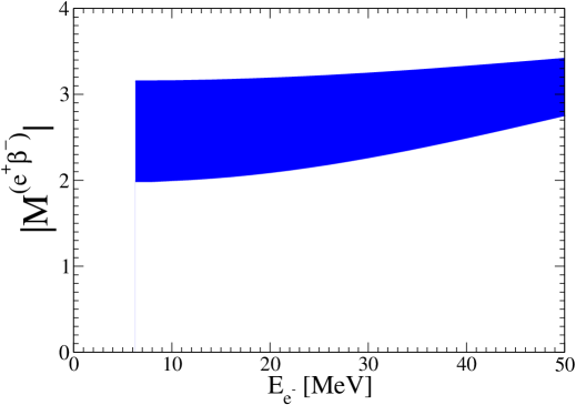
FIG. 1: (Color online) The absolute value of nuclear matrix element ${M}^{(\mathrm{e}\beta^{+})}$ for ⁵⁶Fe as function of energy of incoming electron $E_{\mathrm{e}^{-}}$. The allowed region of calculated nuclear matrix element is determined by fixing the particle–particle parameter to $M^{\nu\overline{\nu}}_{\mathrm{GT}}$ from the range (0, 0.30) MeV^-1.

III Energy production of the reaction $\rm{e}^{-}$ $\rightarrow$ $\rm{e}^{+}$ in the strongly magnetized iron white dwarfs

To estimate the energy production $\bar{\varepsilon}_{r}$ per one event of the reaction (1), we calculated the two-photon positron-electron annihilation probability per volume within the quantum electrodynamics framework W ; BD and integrated it over the energies of electrons $\epsilon_{f}=E_{f}/m_{e}$ interacting with the positron in the final state of the reaction (1) according to the prescription (11). As a result, we obtained

$$\bar{\Gamma_{i}}\,=\,\frac{2\gamma}{(2\pi)^{2}\lambda^{3}_{\mathrm{e}}}\,\int\limits_{1}^{\epsilon_{\,\mathrm{F}}}\,\frac{\epsilon_{f}}{(\epsilon^{2}_{f}-1)^{1/2}}\,\Gamma_{i}\,d\epsilon_{f}\,,\quad i=0,1\ .$$ (48)

Our notations used in this section follow closely those of Chapter 8 in Ref. W . Further,

$$\Gamma_{i}=\frac{(2\pi)^{4}}{8}\,\sum_{\epsilon,\epsilon^{\prime},\,\sigma,\sigma^{\prime}}\,\int\,|M|^{2}\,\delta^{(4)}(p_{f}+p_{\mathrm{e}^{+}}-k-k^{\prime})f_{i}(k^{0}+k^{\prime 0})\,d\bm{k}\,d\bm{k}^{\prime}\,,$$ (49)

$f_{0}(k^{0}+k^{\prime 0})=1$, $f_{1}(k^{0}+k^{\prime 0})=k^{0}+k^{\prime 0}$, the sum is performed over two photon linear polarizations $\epsilon$, $\epsilon^{\prime}$ and the average is done over the electron (positron) spin z-component $\sigma$ ($\sigma^{\prime}$), the final photons have the 4-momenta $k^{\mu}$ and $k^{\prime\mu}$ ($k^{0}=|\bm{k}|=\omega$, $k^{\prime 0}=|\bm{k}^{\prime}|=\omega^{\prime}$), the positron (electron) 4-momentum is $p^{\mu}_{\rm{e}^{+}}$ ($p^{\mu}_{f}$), also $E_{\rm{e}^{+}}=p^{0}_{\rm{e}^{+}}$ and $E_{f}=p^{0}_{f}$. In its turn, the amplitude $M$ is

$$M\, = \,-\frac{e^{2}}{4(2\pi)^{3}\,\sqrt{(}\omega\,\omega^{\prime})}\,{\bar{v}}(\bm{p}_{\rm{e}^{+}},\sigma^{\prime})\left\{\not{\epsilon}^{\prime}[-i(\not{p}_{f}-\not{k})+m_{\mathrm{e}}]\not{\epsilon}\,/(p_{f}\cdot k)\right.$$ (50)

$$\qquad\qquad\qquad\qquad\left.+\not{\epsilon}[-i(\not p_{f}-\not{k}^{\prime})+m_{\mathrm{e}}]\not{\epsilon}^{\prime}\,/(p_{f}\cdot k^{\prime})\right\}u(\bm{p}_{f},\sigma)\,.$$

The calculation of the $|M|^{2}$ reduces to evaluation of traces and yields

$$\Gamma_{i}\, = \,\frac{\alpha^{2}\pi}{2m^{2}_{\mathrm{e}}\epsilon_{\mathrm{e}^{+}}}\,\int\limits_{-1}^{+1}\,dx\,\frac{\bar{\omega}}{\epsilon_{f}+\epsilon_{\mathrm{e}^{+}}+(|\bar{\bm{p}}_{\mathrm{e}^{+}}|-|\bar{\bm{p}}_{f}|)x}\,\left\{\,A_{0}+A_{1}/(\bar{p}_{f}\cdot\bar{k})^{2}\right.$$ (51)

$$\qquad\qquad\qquad\left.\,+A_{2}/(({\bar{p}}_{f}\cdot{\bar{k}})({\bar{p}}_{f}\cdot{\bar{k}^{\prime}}))+A_{3}/({\bar{p}}_{f}\cdot{\bar{k}^{\prime}})^{2}\,\right\}\,m^{i}_{\mathrm{e}}f_{i}(\bar{\omega}+\bar{\omega}^{\prime})\ .$$

Here, the bared quantities are expressed in units of the electron mass and

$$\omega\,=\,\frac{m^{2}_{\mathrm{e}}+E_{\mathrm{e}^{+}}E_{f}-|\bm{p}_{\mathrm{e}^{+}}||\bm{p}_{f}|}{E_{\mathrm{e}^{+}}+E_{f}+(|\bm{p}_{\mathrm{e}^{+}}|-|\bm{p}_{f}|)x}\,,\quad\omega^{\prime}\,=\,E_{\mathrm{e}^{+}}+E_{f}-\omega\ .$$ (52)

The scalar function $A_{0}$ comes from those parts of the traces that do not contain the factors ($\epsilon\cdot p_{f}$) and ($\epsilon^{\prime}\cdot p_{f}$). The functions $A_{i}$, $i=0,1,2,3$, are presented in Appendix A.

In the next step, we include $\bar{\Gamma}_{i}$ into the function $\phi(\epsilon_{\,\mathrm{F}},\gamma)$ , obtaining thus $\phi_{0}(\epsilon_{\,\mathrm{F}},\gamma)$ and $\phi_{1}(\epsilon_{\,\mathrm{F}},\gamma)$ . The energy produced in one event per one second is then calculated as

$$\bar{\varepsilon}_{r}\,=\,\phi_{1}(\epsilon_{\,\mathrm{F}},\gamma)/\phi_{0}(\epsilon_{\,\mathrm{F}},\gamma)\ .$$ (53)

Since the Fermi energy $E_{\,\mathrm{F}}$ of the electron gas is larger than the threshold energy given by the mass difference between the final and the initial nuclei $\Delta^{\beta\beta}_{56}$ plus the positron mass, in average a heat energy in one electron capture event

$$\Delta h=(E_{\,\mathrm{F}}-\Delta^{\beta\beta}_{56}-m_{\mathrm{e}})/2$$ (54)

is released, which should be added to $\bar{\varepsilon}_{r}$.

In the interval of 1 year, the number of reactions in 1 cm³ is $n_{r}=n_{\mathrm{m}}\,\Gamma$, where $n_{\mathrm{m}}$ is the number density of matter. Then the released energy in 1 cm³ per 1 year is

$$E=n_{\mathrm{m}}\,\Gamma\,\bar{\varepsilon}_{r}\ [\mathrm{J}\,\mathrm{cm}^{-3}\,\mathrm{y}^{-1}]\ .$$ (55)

Let us consider the SMIWD with the mass $M_{\mbox{\tiny{SMWD}}}$=2 $M_{\odot}$ $\approx$ 4 $\times\,$10³³ g. Its volume is $V_{\mbox{\tiny{SMWD}}}$=$M_{\mbox{\tiny{SMWD}}}$/$\rho_{\mathrm{m}}$, from which one obtains the radius $R_{\mbox{\tiny{SMWD}}}$. In the full volume, the released energy per 1 year is $EV$ [J y^-1], from which one obtains directly the change in the luminosity (released energy per 1 second) $\Delta L\,=\,EV/3.154\,\times 10^{7}$ W. The influence on the surface temperature of the white dwarf can be calculated from the equation

$$\Delta T\,=\,\left(\frac{\Delta L}{s\,4\pi R_{\mbox{\tiny{SMWD}}}^{2}}\right)^{1/4}\,.$$ (56)

Here, $s=5.67\,\times\,10^{-8}$ W m^-2 K^-4.

The calculated change in the luminosity and in the surface temperature of the SMIWDs is presented in Table 3, obtained by using the necessary input from Table 2, $|\langle m_{\nu}\rangle|$=0.4 eV and Eqs. (43), (44), (47). Besides, $R=1.2A^{1/3}\,\approx\,$ 4.59 fm.

Table 3: The values of the Fermi energy $\epsilon_{\,\mathrm{F}}=E_{\,\mathrm{F}}/m_{\mathrm{e}}$ used in the present study. Further, $R_{\mbox{\tiny{WD}}}$ is the radius of the SMIWD, $\Delta\,L$ is the calculated change in the luminosity, $\Delta\,T$ is the related change in the surface temperature, and the released energy in single reaction, $\bar{\varepsilon}_{r}$ is defined in Eq. (53); the surface temperature of the SMIWD $T_{eff}$ is obtained from Eq. (56), by taking the luminosity $L=10^{-8}\,L_{\odot}$.

$\epsilon_{\,\mathrm{F}}$	$R_{\mbox{\tiny{SMWD}}}$/104 [m]	$\Delta\,L$ [W]	$\Delta\,T$ [K]	$T_{eff}$ [K]	$\bar{\varepsilon}_{r}$ [MeV]
20	42.3	5.9 x 1011	46	2340	15.6
46	18.6	7.4 x 1014	420	3550	44.7

Since neither the luminosity, nor the surface temperature of the SMIWDs are known so far, we estimated possible effect of the reaction (1), given by $\Delta\,T$ in Table 3, on the surface temperature $T_{eff}$, by taking in Eq. (56) the luminosity $L=10^{-8}\,L_{\odot}$, where the solar luminosity $L_{\odot}$= 3.828 $\times$ 10²⁶ W PDG . These estimates indicate that the change in the temperature can be as large as 10 % of $T_{eff}$. However, as is seen from the values of $T_{eff}$, such objects are too dim to be observed.

In Table 4, we present the ratio of the calculated change in the luminosity $\Delta\,L$ of the SMIWDs to the solar luminosity $L_{\odot}$, employing again the necessary input from Table 2, $|\langle m_{\nu}\rangle|$=0.4 eV and 0.8 eV, and $R=1.2A^{1/3}\,\approx\,$ 4.59 fm.

Table 4: The values of the Fermi energy $\epsilon_{\,\mathrm{F}}$=$E_{\,\mathrm{F}}/m_{\mathrm{e}}$ used in the present study. Further, $(\Delta L/L_{\odot})_{0.4}$ and $(\Delta L/L_{\odot})_{0.8}$ are the ratios of the change in the luminosity of the SMIWD due to the reaction (1) to the luminosity of the Sun, calculated for $|\langle m_{\nu}\rangle|$=0.4 eV and 0.8 eV, respectively.

$\epsilon_{\,\mathrm{F}}$	$\left[Log(\Delta L/L_{\odot})\right]_{0.4}$	$\left[Log(\Delta L/L_{\odot})\right]_{0.8}$
20	-14.8	-14.2
46	-11.7	-11.1

In the next section, we discuss the cooling of white dwarfs and compare our results with the existing cooling models.

IV Cooling of white dwarfs

The basic model of cooling of the WDs was formulated by Mestel ST ; LM . In this model, the thin surface layer is considered as non-degenerate, whereas the interior of the WDs is taken as fully degenerate. The accumulated heat energy of the core is transported to the surface by diffusion of photons and electrons.

Concerning the cooling of the SMWDs, to our knowledge, no specific calculations were performed till now. Various processes occurring in the plasma under the influence of a strong magnetic field were studied already 40 years ago in Refs. CCh ; FC ; CC ; CCC ; CLR and recently reviewed in Ref. AYPA .

In order to estimate qualitatively possible effect of the reaction (1) on the cooling of the SMIWDs, we suggested that the correctly calculated cooling process would be similar as for the iron-core WDs. Extrapolating the data, presented in Fig. 17 PAB for the curve corresponding to $M/M_{\odot}$=0.6 to smaller values of the luminosity, we got that $Log(L/L_{\odot})\,\approx\,$-5.0 (-7.54) is achieved after the cooling time $\tau\,\approx\,$3.48 (3.90) Gyr . It is clear from Table 4 that the effect of the double charge exchange reaction (1) could influence the luminosity only in the asymptotic region. Since the inverse beta-decay should be taken into account in the study of the SMIWDs as well, it follows from Refs. BK1 ; BS ; BK2 that the effect of the reaction (1) on the asymptotic will be combined with the non-equilibrium heat from the second part of the reaction (7).

V SMIWDs as SGRs/AXPs

During the last decade the observational astrophysics made substantial progress in the study of the SGR- and AXP sources of the radiation MCG . These compact objects are standardly identified with magnetars, that are a class of the NSs powered by strong magnetic fields up to 10¹⁵ G. In the last years, SGRs/AXPs with lower magnetic fields of the order $\sim$ 10¹²-10¹³ G and with the rotation period P $\sim$ 10 s have been observed. It was shown in Refs. MRR ; CM ; BIRR that these fast rotating magnetized NSs can be alternatively described as massive fast rotating magnetized WDs. Here we show that similar description is possible within the concept of the fast rotating SMIWDs. Below we follow closely the notations of Section 2 CM .

The magnetic moment of the rotating star can be expressed in terms of the observables such as the rotational period $P$ and the spin-down rate $\stackrel{{\scriptstyle.}}{{P}}$ as

$$m=\left(\frac{3c^{3}I}{8\pi^{2}}\,P{\stackrel{{\scriptstyle.}}{{P}}}\right)^{1/2}\,,$$ (57)

where $I$ is the momentum of inertia. Besides, the surface magnetic field at the equator is

$$B_{e}=\frac{m}{R^{3}}\,,$$ (58)

where $R$ is the radius of the star at the equator.

In this pulsar model, the X-ray luminosity is supposed to come fully from the loss of the rotational energy

$$\stackrel{{\scriptstyle.}}{{E}}_{rot}=-4\pi^{2}I\frac{\stackrel{{\scriptstyle.}}{{P}}}{P^{3}}\,,$$ (59)

and the characteristic age of the pulsar is

$$\tau=\frac{P}{2\stackrel{{\scriptstyle.}}{{P}}}\,.$$ (60)

In the case of the magnetar model DT ; TAD , the choice for the mass of the NS is $M=1.4M_{\odot}$ and $R$ = 10 km, whereas in the WD model MRR ; CM ; BIRR , $M=1.4M_{\odot}$ and $R$ = 3000 km.

In the approach of the SMIWDs we take $M=2M_{\odot}$ and the radii from our Table 3. Next we analyze the data for the magnetars SGR 0418+579 and Swift J1822.6-1606.

a) SGR 0418+5729

$$P(s) = 9.0784\,\,^{a})\,,\quad\stackrel{{\scriptstyle.}}{{P}}(s\,s^{-1})=4\times 10^{-15}\,\,{}^{a})\,,\quad d=2\,{\rm kpc}\,^{a})\,\,,$$

$$\Delta L_{X} = 7.5\times 10^{-15}\,{\rm erg\,s}^{-1}{\rm cm}^{-2}\,{}^{b})\,\,.$$ (61)

^a)  Ref. RSGR  , ^b)  Ref. RPC

From $\Delta L_{X}$ and the distance $d$ of Eq. (61) one obtains for the total luminosity and the age

$$L_{X}=3.6\times 10^{30}{\rm ergs}^{-1}\,,\quad\tau=36\,{\rm Myr}\,.$$ (62)

Using Eqs. (57)-(60) and the data (61) one arrives at the results

$$m_{\tiny{NS}}=6.4\times 10^{30}\,{\rm emu}\,,\quad B_{\tiny{NS}}=6.4\times 10^{12}\,{\rm G}\,,\quad|\stackrel{{\scriptstyle.}}{{E}}_{\tiny{rot}}^{\tiny{NS}}|=7.5\times 10^{28}{\rm erg\,s}^{-1}\,,$$ (63)

$$m_{\tiny{WD}}=1.9\times 10^{33}\,{\rm emu}\,,\quad B_{\tiny{WD}}=7.1\times 10^{7}\,{\rm G}\,,\quad|\stackrel{{\scriptstyle.}}{{E}}_{\tiny{rot}}^{\tiny{WD}}|=6.7\times 10^{33}{\rm erg\,s}^{-1}\,.$$ (64)

Table 5: The values of the magnetic moment $m_{\tiny{SMIWD}}$ (in emu), of the flux of the magnetic field $B_{\tiny{SMIWD}}$ (in G) and of the rotational energy $|\stackrel{{\scriptstyle.}}{{E}}_{\tiny{rot}}^{\tiny{SMIWD}}|$ (in erg s^-1) for the compact object SGR 0418+5729, considered as a fast rotating SMIWD.

$R_{\mbox{{\tiny{SMIWD}}}}$ [km]	423	186
$m_{\mbox{{\tiny{SMIWD}}}}/10^{31}$	32.5	14.3
$B_{\mbox{{\tiny{SMIWD}}}}/10^{10}$	0.43	2.22
$|\stackrel{{\scriptstyle.}}{{E}}_{\tiny{rot}}^{\tiny{SMIWD}}|/10^{30}$	191	37

Comparing the results for the rotational energy, presented in Table 5, with the total luminosity (62) one can see that the loss of this energy of the SMIWDs can explain $L_{X}$. As is seen from Eq. (64), this is also true for the fast rotating WD. On the contrary, the loss of the rotational energy of the NS (63) is by about two orders of the magnitude smaller than (62).

b) Swift J1822.6-1606

The data below are taken from Ref. RSWIFT :

$$P(s) = 8.4377\,\,,\quad\stackrel{{\scriptstyle.}}{{P}}(s\,s^{-1})=8.3\times 10^{-14}\,\,,\quad d=5\,{\rm kpc}\,,$$

$$\Delta L_{X} = 4\times 10^{-14}\,{\rm erg\,s}^{-1}{\rm cm}^{-2}\,.$$ (65)

From $\Delta L_{X}$ and the distance $d$ of Eq. (65) one obtains for the total luminosity and the age

$$L_{X}=1.2\times 10^{32}{\rm ergs}^{-1}\,,\quad\tau=1.61\,{\rm Myr}\,.$$ (66)

Using Eqs. (57)-(60) and the data (65) one arrives at the results

$$m_{\tiny{NS}}=2.8\times 10^{31}\,{\rm emu}\,,\quad B_{\tiny{NS}}=2.8\times 10^{13}\,{\rm G}\,,\quad|\stackrel{{\scriptstyle.}}{{E}}_{\tiny{rot}}^{\tiny{NS}}|=1.9\times 10^{30}{\rm erg\,s}^{-1}\,,$$ (67)

$$m_{\tiny{WD}}=8.5\times 10^{33}\,{\rm emu}\,,\quad B_{\tiny{WD}}=3.1\times 10^{8}\,{\rm G}\,,\quad|\stackrel{{\scriptstyle.}}{{E}}_{\tiny{rot}}^{\tiny{WD}}|=1.7\times 10^{35}{\rm erg\,s}^{-1}\,.$$ (68)

Table 6: The values of the magnetic moment $m_{\tiny{SMIWD}}$ (in emu), of the flux of the magnetic field $B_{\tiny{SMIWD}}$ (in G) and of the rotational energy $|\stackrel{{\scriptstyle.}}{{E}}_{\tiny{rot}}^{\tiny{SMIWD}}|$ (in erg s^-1) for the compact object Swift J1822.6-1606, considered as a fast rotating SMIWD.

$R_{\mbox{{\tiny{SMIWD}}}}$ [km]	423	186
$m_{\mbox{{\tiny{SMIWD}}}}/10^{32}$	14.3	6.28
$B_{\mbox{{\tiny{SMIWD}}}}/10^{11}$	0.19	0.98
$|\stackrel{{\scriptstyle.}}{{E}}_{\tiny{rot}}^{\tiny{SMIWD}}|/10^{32}$	49.4	9.6

Comparing the results for the rotational energy, presented in Table 6, with the total luminosity (66) one can see, as in the case of SGR 0418+5729, that the loss of this energy of the SMIWDs can explain $L_{X}$. As is seen from Eq. (68), this is also true for the fast rotating WD. On the contrary, the loss of the rotational energy of the NS (67) is by about two orders of the magnitude smaller than (62).

On the other hand, comparison of the rotational energies of Table 5 and Table 6 with the 3rd column of Table 3 shows that the energy produced by the reaction of the double charge exchange (2) cannot influence sizeably the luminosity of the compact objects considered above as fast rotating SMIWDs.

VI Discussion of the results and conclusions

In this work, we studied the influence of the double charge exchange reaction (1) on the cooling of the SMIWDs. This reaction is closely related to the neutrinoless double beta-decay process, which is nowadays studied intensively VES . Both processes violate the lepton number by two units and, therefore, take place if and only if the neutrinos are the Majorana particles with the non-zero mass. For the case of light neutrino exchange, the $(\mathrm{e}^{-},\mathrm{e}^{+})$ conversion and the $0\nu\beta\beta$-decay rates are proportional to the squared absolute value of the effective mass of the Majorana neutrinos, $|\langle m_{\nu}\rangle|^{2}$.

Our study is based on the theory of the SMWDs KM ; DM ; DM1 ; DM2 . This theory, when applied to the phenomenon of the Ia supernovae, can reasonably explain the existence of the observed progenitor star with the mass exceeding the CL limit DM3 ; DM4 . Our model calculations are done for the case of the SMIWDs, in which the magnetic field is strong enough to maintain the Fermi energy of the electron sea larger than the threshold energy for the reaction (1), which is 6.33 MeV. We considered $\epsilon_{\,\mathrm{F}}=E_{\,\mathrm{F}}/m_{\mathrm{e}}$=20, 46, and have chosen the strength of the magnetic field so that the value of the related parameter $\gamma={\cal B}/{\cal B}_{c}$ allowed us to restrict ourselves to the ground Landau level.

The calculations are first performed under the assumption that the SMIWDs radiate in the visible spectrum. The results are presented in Table 3 and Table 4.

In calculating Table 3, we suggested that an SMIWD can possess the luminosity of the size $L=10^{-8}L_{\odot}$ and obtained the corresponding surface temperature from Eq. (56). Then the comparison with the calculated effect of the reaction (1) shows possible influence of 10 %. However, as is seen from the values of $T_{eff}$, such objects would be too dim to be observed.

Since the theory of cooling of the SMIWDs has not yet been developed, we turned to the one for the iron-core WDs, which is well elaborated. By comparing the luminosity of the pure iron-core DA models of Fig. 17 PAB with our Table 4 we can conclude that the double charge exchange reaction (1) could in the case of the SMIWDs retard their cooling at low luminosity by pumping over the energy of the Fermi sea of electrons to the thermal energy of ions. However, the effect would be out of reach of the present observational possibilities. Moreover, it would be diminished by the non-equilibrium heat from the inverse beta-decay reaction (7) BK1 ; BS ; BK2 .

Then in Section V, we explored the SMIWDs as fast rotating stars that can be considered as GSR/AXPs. We have shown ( see Table 5 and Table 6) that using the observational data for the magnetars SGR 0418+579 and Swift J1822.6-1606, the calculated loss of the rotational energy can reproduce the observed total luminosity for the considered SWIMDs. However, the energy produced by the reaction of the double charge exchange (2) cannot influence sizeably the luminosity of the compact objects considered as fast rotating SMIWDs.

Our main conclusion is that the energy, released in reaction (1), (i) could influence under certain assumption the effective temperature up to 10 %, but the SWIMDs would be too dim to be observed at present; (ii) could retard cooling of the SMIWDs at sufficiently low luminosity, which seem to be, however, at an unobservable level at present as well; (iii) cannot influence sizeably the luminosity of these compact objects considered as the sources of SGR/AXP radiation. It means that the study of the double charge exchange reaction (1) in the SMIWDs using simple model KM ; DM ; DM1 ; DM3 ; DMR with the ground Landau level and at the present level of accuracy of measurement of the luminosity and energy of the cosmic gamma-rays could not provide conclusive information on the Majorana nature of the neutrino, if its effective mass would be $|\langle m_{\nu}\rangle|$ $\leq$ 0.8 $eV$.

Appendix A Calculations of traces

Here we provide the invariant functions $A_{i}$ entering the positron-electron annihilation probability (51), resulting from calculations of traces and summing over the photon linear polarizations. The calculations are made in the Coulomb gauge, putting $\epsilon^{0}$=$\epsilon^{\prime 0}$=0 and using

$$\sum_{\epsilon}\epsilon_{i}\epsilon_{j}\,=\,\delta_{ij}-\hat{\bm{k}}_{i}\hat{\bm{k}}_{j}\,,\quad\sum_{\epsilon^{\prime}}\epsilon^{\prime}_{i}\,\epsilon^{\prime}_{j}\,=\,\delta_{ij}-\hat{\bm{k}}^{\prime}_{i}\hat{\bm{k}}^{\prime}_{j}\,.\\$$

$$m^{4}_{\mathrm{e}}A_{0}\,=\,\frac{(k\cdot k^{\prime})^{2}}{(p_{f}\cdot k)(p_{f}\cdot k^{\prime})}-a_{0}\,,$$ (69)

$$m^{4}_{\mathrm{e}}A_{1}\,=\,\left\{(-a_{3}+a_{5}+a_{11})(p_{f}\cdot k)+[\,(p_{f}\cdot k^{\prime})-(k\cdot k^{\prime})+a_{1}-a_{2}\,]a_{13}\right\}/(p\cdot k)^{2}\,,$$ (70)

$$m^{4}_{\mathrm{e}}A_{2}\, = \,\left\{[a_{1}-a_{4}+a_{12}-a_{13}+(a_{8}-a_{6})/2](p_{f}\cdot k)+\left[a_{3}-a_{10}-a_{11}+a_{12}\right.\right.$$ (71)

$$\left.\left.\,+(a_{6}-a_{8})/2\right](p_{f}\cdot k^{\prime})+[-a_{1}-a_{3}+a_{4}+a_{11}-a_{12}+(a_{5}+a_{7})/2](k\cdot k^{\prime})\right.$$

$$\left.\,+(a_{9}-a_{3})a_{11}+(a_{13}-a_{4})a_{1}+a_{3}a_{10}\right\}/(p_{f}\cdot k)(p_{f}\cdot k^{\prime})\,,$$

$$m^{4}_{\mathrm{e}}A_{3}\,=\,\left\{[\,(p_{f}\cdot k)-(k\cdot k^{\prime})+a_{3}-a_{9}\,]a_{10}+(-a_{1}+a_{4}+a_{7})(p_{f}\cdot k^{\prime})\right\}/(p_{f}\cdot k^{\prime})^{2}\,.$$ (72)

Further,

$$a_{0}\,=\,1+(\hat{\bm{k}}\cdot\hat{\bm{k}}^{\prime})^{2}\,,$$ (73)

$$a_{1}\,=\,(\bm{p}_{f}\cdot\bm{p}_{\mathrm{e}^{+}})-(\bm{p}_{f}\cdot\hat{\bm{k}}^{\prime})(\bm{p}_{\mathrm{e}^{+}}\cdot\hat{\bm{k}}^{\prime})\,,$$ (74)

$$a_{2}\,=\,(\bm{p}_{\mathrm{e}^{+}}\cdot\hat{\bm{k}})-(\bm{p}_{\mathrm{e}^{+}}\cdot\hat{\bm{k}}^{\prime})(\hat{\bm{k}}\cdot\hat{\bm{k}}^{\prime})\,,$$ (75)

$$a_{3}\,=\,(\bm{p}_{f}\cdot\bm{p}_{\mathrm{e}^{+}})-(\bm{p}_{f}\cdot\hat{\bm{k}})(\bm{p}_{\mathrm{e}^{+}}\cdot\hat{\bm{k}})\,,$$ (76)

$$a_{4}\,=\,(\bm{p}_{f}\cdot\hat{\bm{k}}^{\prime})-(\bm{p}_{f}\cdot\hat{\bm{k}})(\hat{\bm{k}}\cdot\hat{\bm{k}}^{\prime})\,,$$ (77)

$$a_{5}\,=\,(\bm{p}_{f}\cdot\bm{p}_{\mathrm{e}^{+}})-(\bm{p}_{f}\cdot\hat{\bm{k}})(\bm{p}_{\mathrm{e}^{+}}\cdot\hat{\bm{k}})-(\bm{p}_{f}\cdot\hat{\bm{k}}^{\prime})(\bm{p}_{\mathrm{e}^{+}}\cdot\hat{\bm{k}}^{\prime})+(\bm{p}_{f}\cdot\hat{\bm{k}})(\bm{p}_{\mathrm{e}^{+}}\cdot\hat{\bm{k}}^{\prime})(\hat{\bm{k}}\cdot\hat{\bm{k}}^{\prime})\,,$$ (78)

$$a_{6}\,=\,(\hat{\bm{k}}\cdot\hat{\bm{k}}^{\prime})\left[-(\bm{p}_{f}\cdot\hat{\bm{k}}^{\prime})+(\bm{p}_{f}\cdot\hat{\bm{k}})(\hat{\bm{k}}\cdot\hat{\bm{k}}^{\prime})\right]\,,$$ (79)

$$a_{7}\,=\,(\bm{p}_{f}\cdot\bm{p}_{\mathrm{e}^{+}})-(\bm{p}_{f}\cdot\hat{\bm{k}})(\bm{p}_{\mathrm{e}^{+}}\cdot\hat{\bm{k}}^{\prime})-(\bm{p}_{f}\cdot\hat{\bm{k}}^{\prime})(\bm{p}_{\mathrm{e}^{+}}\cdot\hat{\bm{k}}^{\prime})+(\bm{p}_{f}\cdot\hat{\bm{k}}^{\prime})(\bm{p}_{\mathrm{e}^{+}}\cdot\hat{\bm{k}})(\hat{\bm{k}}\cdot\hat{\bm{k}}^{\prime})\,,$$ (80)

$$a_{8}\,=\,(\hat{\bm{k}}\cdot\hat{\bm{k}}^{\prime})\left[-(\bm{p}_{f}\cdot\hat{\bm{k}})+(\bm{p}_{f}\cdot\hat{\bm{k}}^{\prime})(\hat{\bm{k}}\cdot\hat{\bm{k}}^{\prime})\right]\,,$$ (81)

$$a_{9}\,=\,(\bm{p}_{\mathrm{e}^{+}}\cdot\hat{\bm{k}}^{\prime})-(\bm{p}_{\mathrm{e}^{+}}\cdot\hat{\bm{k}})(\hat{\bm{k}}\cdot\hat{\bm{k}}^{\prime})\,,$$ (82)

$$a_{10}\,=\,\bm{p}_{f}^{2}-(\bm{p}_{f}\cdot\hat{\bm{k}}^{\prime})^{2}\,,$$ (83)

$$a_{11}\,=\,(\bm{p}_{f}\cdot\bm{k})-(\bm{p}_{f}\cdot\hat{\bm{k}}^{\prime})(\bm{k}\cdot\hat{\bm{k}}^{\prime})\,,$$ (84)

$$a_{12}\,=\,\bm{p}_{f}^{2}-(\bm{p}_{f}\cdot\hat{\bm{k}})^{2}-(\bm{p}_{f}\cdot\hat{\bm{k}}^{\prime})^{2}+(\bm{p}_{f}\cdot\hat{\bm{k}})(\bm{p}_{f}\cdot\hat{\bm{k}}^{\prime})(\hat{\bm{k}}\cdot\hat{\bm{k}}^{\prime})\,,$$ (85)

$$a_{13}\,=\,\bm{p}_{f}^{2}-(\bm{p}_{f}\cdot\hat{\bm{k}})^{2}\,.$$ (86)

Here, ${\hat{\bm{a}}}=\bm{a}/|\bm{a}|$ is the unit vector. The invariant function $A_{0}$ arises from the part of traces that do not contain the factors $(\epsilon\cdot p_{f})$ and $(\epsilon^{\prime}\cdot p_{f})$. If one puts $\bm{p}_{f}=0$, one obtains the positron-electron annihilation probability in the laboratory frame of reference. At threshold positron energies one gets for $\Gamma_{0}$

$$\Gamma_{0}\,=\,\frac{\alpha^{2}\pi}{m_{\mathrm{e}}^{2}}\,,$$ (87)

which provides for the annihilation cross section

$$\sigma\,=\,\frac{\alpha^{2}\pi}{vm_{\mathrm{e}}^{2}}\,,$$ (88)

where $v$ is the positron velocity.

References

- (1) Y. Terada, Thirteenth Marcel Grossmann Meeting, summary of the session ’White dwarf pulsars and rotating white dwarf theory’, arXiv: 1306.4053.
- (2) D. Koestler, G. Chanmugam, Rep. Prog. Phys. 53 (1990) 837.
- (3) B. Hansen, Phys. Rep. 399 (2004) 1.
- (4) L.G. Althaus, A.H. Córsico, J. Isern, E. Garcia-Berro, Astron. Astrophys. Rev. 18(4) (2010) 471-566.
- (5) J. Isern, S. Catalan, E. Garcia-Berro, M. Lalaris, S. Torres, in: L. Baudis, M. Schumann (Eds.), Proc. of the 6th Patras Workshop on Axions, WIMPs and WISPs, Hamburg, DESY, 2010, p.77-80.
- (6) J. Isern, E. Garcia-Berro, S. Torres, S. Catalan, Astrophys. J. Lett. 682 (2008) L109.
- (7) J.D. Vergados, H. Ejiri, F. Šimkovic, Rep. Prog. Phys. 75 (2012) 106301.
- (8) M. Agostini et al. Phys. Rev. Lett. 111 (2013) 122503.
- (9) S.R. Elliot et al. (MAJORANA Collaboration), AIP Conf. Proc. 1572 (2013) 48.
- (10) E.E. Salpeter, Astrophys. J. 134 (1961) 669.
- (11) S.L. Shapiro, S.A. Teukolsky, Black Holes, White Dwarfs, and Neutron Stars: The Physics of Compact Objects, Wiley, New York, 1983.
- (12) M. Rotondo, J.A. Rueda, R. Ruffini, S. -S. Xue, Phys. Rev. D 84 (2011) 084007.
- (13) G.S. Bisnovatyi-Kogan, Stellar Physics 1: Fundamental Concepts and Stellar Equilibrium, Springer, 2001.
- (14) G.S. Bisnovatyi-Kogan, Z.F. Seidov, Sov. Astron., A.J. 47 (1970) 139.
- (15) G. Audi, A.H. Wapstra, C. Thibault, Nucl. Phys. A 729 (2003) 337.
- (16) J.A. Panei, L.G. Althaus, O.G. Benvenuto, Mon. Not. R. Astron. Soc. 312 (2000) 531.
- (17) G.S. Bisnovatyi-Kogan, Stellar Physics 2: Stellar Evolution and Stability, Springer, 2010.
- (18) M.P. Savedoff, H.M. Van Horn, S.C. Vilas, Astrophys. J. 155 (1969) 221.
- (19) J.L. Provencal, H.L. Shipman, E. Hog, P. Thejll, Astrophys. J. 494 (1998) 759.
- (20) H.L. Shipman, J.L. Provencal, ASP Conf. Series 169 (1999) 15.
- (21) J.L. Provencal, H.L. Shipman, D. Koester, F. Wesemael, P. Bergeron, Astrophys. J. 568 (2002) 324.
- (22) G. Fontaine, F. Bergeron, P. Brassard, ASP Conf. Series 372 (2007) 13.
- (23) M.A. Barstow et al., White paper: Gaia and the end states of stellar evolution, arXiv:1407.6163.
- (24) J. Isern, R. Canal, J. Labay, Astrophys. J. 372 (1991) L83.
- (25) R. Ouyed, J. Staff, P. Jaikumar, Astrophys. J. 743 (2011) 116.
- (26) G.J. Mathews, I.S. Suh,B. O’Gorman, N.Q. Lan, W. Zach, K. Otsuki, F. Weber, J. Phys. G, Nucl. Part. Phys. 32 (2006) 747.
- (27) A.Y. Potekhin, Phys. Usp. 53 (2010) 1235.
- (28) S. Catalan, I. Ribas, J. Isern, E. Garcia-Berro, Astron. Astrophys. 477 (2008) 901.
- (29) P. Bera, D. Bhattacharya, Mon. Not. R. Astron. Soc. 445 (2014) 3951.
- (30) U. Das, B. Mukhopadhyay, GRMHD formulation of highly super-Chandrasekhar magnetized white dwarfs: stable configurations of non-spherical white dwarfs, arXiv:1411.5367.
- (31) A. Kundu, B. Mukhopadhyay, Mod. Phys. Lett. A 27 (2012) 1250084.
- (32) U. Das, B. Mukhopadhyay, Phys. Rev. D 86 (2012) 042001.
- (33) U. Das, B. Mukhopadhyay, Int. J. Mod. Phys. D 21 (2012) 1242001.
- (34) U. Das, B. Mukhopadhyay, Mod. Phys. Lett. A 29 (2014) 1450035.
- (35) L.D. Landau, E.M. Lifshits, Quantum Mechanics, State Publishing House of Physical and Mathematical Literature, Moscow, 1963 (in Russian).
- (36) M. Strickland, V. Dexheimer, D.P. Menezes, Phys. Rev. D 86 (2012) 125032.
- (37) D. Lai, S.I. Shapiro, Astrophys. J. 383 (1991) 745.
- (38) I. Bednarek, A. Brzezina, R. Manka, M. Zastawny-Kubica, Astron. Nachr. 324 (2003) 425.
- (39) R. Manka, M. Zastawny-Kubica, A. Brzezina, I. Bednarek, arXiv:astro-ph/0112512.
- (40) I.S. Suh, G.M. Mathews, Astrophys. J. 530 (2000) 949.
- (41) J.M. Wilkes, R.L. Ingraham, Astrophys. J. 344 (1989) 399.
- (42) S. Chandrasekhar, Astrophys. J. 74 (1931) 81.
- (43) L.D. Landau, Phys. Z. Sowjetunion 1 (1932) 285.
- (44) Y. Kamiya, M. Tanaka, K. Nomoto, S.I. Blinnikov, E.I. Sorokina, T. Suzuki, Astrophys. J. 756 (2012) 191.
- (45) I. Hachisu, M. Kato, H. Saio, K. Nomoto, Astrophys. J. 744 (2012) 69.
- (46) K. Boshkayev, J. Rueda, R. Ruffini, Int. J. Mod. Phys. E 20 (2011) 136.
- (47) K. Boshkayev, J.A. Rueda, R. Ruffini, I. Siutsou, Astrophys. J. 762 (2012) 117.
- (48) U. Das, B. Mukhopadhyay, Phys. Rev. Lett. 110 (2013) 071102.
- (49) U. Das, B. Mukhopadhyay, A.R. Rao, Astrophys. J. Lett. 767 (2013) L14, 5pp.
- (50) P.C.C. Freire, T.M. Tauris, Mon. Not. R. Astron. Soc. 438 (2014) 86.
- (51) R. Nityanada, S. Konar, Phys. Rev. D 89 (2014) 103017.
- (52) N. Chamel, A.F. Fantina, P.J. Davis, Phys. Rev. D 88 (2013) 081301(R).
- (53) N. Chamel, E. Molter, A.F. Fantina, D. Pena Arteaga, Phys. Rev. D 90 (2014) 043002.
- (54) J.G. Coelho et al., Astrophys. J. 794 (2014) 86.
- (55) U. Das, B. Mukhopadhyay, Comment on ”Strong constraints on magnetized white dwarfs surpassing Chandrasekhar mass limit”, arXiv: 1406.0948.
- (56) S. Chandrasekhar, E. Fermi, Astrophys. J. 118 (1953) 116.
- (57) V.C.A. Ferraro, Astrophys. J. 119 (1954) 407.
- (58) M. Bocquet, S. Bonazzola, E. Gourgoulhon, J. Novak, Astron. Astrophys. 301 (1995) 757.
- (59) U. Das, B. Mukhopadhyay, J. Cosmol. Astropart. Phys. 06 (2014) 050.
- (60) A.G. Pili, N. Bucciantini, L. Del Zanna, Int. J. Mod. Phys. Conf. Ser. 28 (2014) 1460202.
- (61) R.J. Tayler, Mon. Not. R. Astron. Soc. 161 (1973) 365.
- (62) R. Ciolfi, L. Rezzolla, Mon. Not. R. Astron. Soc. 435 (2013) L43.
- (63) R. Ciolfi, Astron. Nachr. 335 (2014) 285.
- (64) J.P. Ostriker, F.D.A. Hartwick, Astrophys. J. 153 (1968) 797.
- (65) A. Mathew, M.K. Nandy, General relativistic calculations for white dwarfs stars, arXiv: 1401.0819.
- (66) L. Herrera, W. Baretto, Phys. Rev. D 88 (2013) 084022.
- (67) J.M. Dong, W. Zuo, P. Yin, J.Z. Gu, Phys. Rev. Lett. 112 (2014) 039001.
- (68) A.Y. Potekhin, D.G. Yakovlev, Phys. Rev. C 85 (2013) 039801.
- (69) V. Dexheimer, D.P. Menezes, M. Strickland, J. Phys. G, Nucl. Part. Phys. 41 (2014) 015203.
- (70) D. Chatterjee, T. Elghozi, J. Novak, M. Oertel, Consistent neutron star models with magnetic field dependent equation of state, arXiv:1410.6332.
- (71) Y. Tomimura, Y. Eriguchi, Mon. Not. R. Astron. Soc. 359 (2005) 1117.
- (72) S.K. Lander, D.I. Jones, Mon. Not. R. Astron. Soc. 395 (2009) 2162.
- (73) N. Bucciantini, L. Del Zanna, Astron. Astrophys. 528 (2011) A101.
- (74) A.G. Pili, N. Bucciantini, L. Del Zanna, Mon. Not. R. Astron. Soc. 439 (2014) 3541.
- (75) T.M. Tauris, D. Sanyal, S.C. Yoon, N. Langer, Astron. Astrophys. 558 (2013) A39, 25pp.
- (76) S.G. Parsons et al., Mon. Not. R. Astron. Soc. 436 (2013) 241.
-
(77)
M. Dan, S. Rosswog, M. Brüggen, P. Podsiadlowski,
Mon. Not. R. Astron. Soc. 438 (2014) 14. - (78) K. Kashiyama, K. Ioka, P. Mészáros, Astrophys. J. Lett. 776 (2013) L39, 4pp.
- (79) M. Ilkov, N. Soker, Mon. Not. R. Astron. Soc. 419 (2012) 1695.
- (80) J.A Rueda et al., Astrophys. J. Lett. 772 (2013) L24, 4pp.
- (81) M. Malheiro, J.G. Coelho, Describing SGRs/AXPs as fast and magnetized white dwarfs, arXiv:1307.5074.
- (82) M. Malheiro, J.A. Rueda, R. Ruffini, Publ. Astron. Soc. Jpn. 64 (2012) 56.
- (83) J.G. Coelho, M. Malheiro, Publ. Astron. Soc. Jpn. 66 (2014) 1.
- (84) K. Boshkayev, L. Izzo, J.A. Rueda, R. Ruffini, Astron. Astrophys. 555 (2013) A151.
- (85) R.C. Duncan, C. Thompson, Astrophys. J. Lett. 392 (1992) L9.
- (86) C. Thompson, R.C.Duncan, Mon. Not. R. Astron. Soc. 275 (1995) 255.
- (87) N.R. Ikhsanov, N.G. Beskrovnaya, Formation and appearance of pulsar-like white dwarfs, arXiv: 1401.5374.
- (88) P. Ruiz-Lapuente, New Astron. Rev. 62-63 (2014) 15.
- (89) K. Postnov, L. Yungelson, Living Rev. Relativity 17 (2014) 3.
- (90) B. Külebi, J. Kalirai, S. Jordan, F. Euchner, Astron. Astrophys. 554 (2013) A18.
- (91) S.O. Kepler et al., Mon. Not. R. Astron. Soc. 429 (2013) 2934.
- (92) A.Y. Potekhin, Phys. Usp. 57 (2014) 735.
- (93) S.A. Olausen, V.M. Kaspi, Astrophys. J. Suppl. 212 (2014) 6.
- (94) N. Rea et al., Astrophys. J. 770 (2013) 65.
- (95) N. Rea, personal communication, 2013.
- (96) N. Rea et al., Astrophys. J. 754 (2012) 27.
- (97) L. Baudis et al., Phys. Rev. Lett. 83 (1999) 41.
- (98) C. Arnaboldi et al. (CUORE Collaboration), Phys. Lett. B 584 (2004) 260.
- (99) A. Gando et al. (KamLAND-Zen Collaboration), Phys. Rev. C 85 (2012) 045504.
- (100) F. Šimkovic, A. Faessler, H. Müther, V. Rodin, M. Stauf, Phys. Rev. C 79 (2009) 055501.
- (101) H.V. Klapdor-Kleingrothaus, I.V. Krivosheina, Mod. Phys. Lett. A 21 (2006) 1547.
- (102) F.T. Avignone, S.R. Elliott, J. Engel, Rev. Mod. Phys. 80 (2008) 481.
- (103) M. Doi, T. Kotani, E. Takasugi, Prog. Theor. Phys. Suppl. 83 (1985) 1.
- (104) F. Šimkovic, A. Faessler, V.A. Rodin, P. Vogel, J. Engel, Phys. Rev. C 77 (2008) 045503.
- (105) R. Machleidt, Phys. Rev. C 63 (2001) 024001.
- (106) S. Weinberg, The Quantum Theory of Fields, v. I, Cambridge University Press, 1995.
- (107) J.D. Bjorken, S.D. Drell, Relativistic Quantum Mechanics, v. I, McGraw-Hill, 1964.
- (108) J. Beringer et al., Phys. Rev. D 86 (2012) 010001.
- (109) L. Mestel, Mon. Not. R. Astron. Soc. 112 (1952) 583.
- (110) V. Canuto, H.Y. Chiu, Phys. Rev. 173 (1968) 1210; Phys. Rev. 173 (1968) 1220; Phys. Rev. 173 (1968) 1229; Phys. Rev. 188 (1969) 2446.
- (111) L. Fassio-Canuto, Phys. Rev. 187 (1969) 2141.
- (112) V. Canuto, C. Chiuderi, Phys. Rev. D 1 (1970) 2219.
- (113) V. Canuto, H.Y. Chiu, C.K. Chou, Phys. Rev. D 2 (1970) 281.
- (114) V. Canuto, J. Lodenquai, M. Ruderman, Phys. Rev. D 3 (1971) 2301.