Numerical simulation of the Tayler instability in liquid metals

Abstract

The electrical current through an incompressible, viscous and resistive liquid conductor produces an azimuthal magnetic field that becomes unstable when the corresponding Hartmann number exceeds a critical value in the order of 20. This Tayler instability, which is not only discussed as a key ingredient of a non-linear stellar dynamo model (Tayler-Spruit dynamo), but also as a limiting factor for the maximum size of large liquid metal batteries, was recently observed experimentally in a column of a liquid metal [1]. On the basis of an integro-differential equation approach, we have developed a fully three-dimensional numerical code, and have utilized it for the simulation of the Tayler instability at typical viscosities and resistivities of liquid metals. The resulting growth rates are in good agreement with the experimental data. We illustrate the capabilities of the code for the detailed simulation of liquid metal battery problems in realistic geometries.

1 Introduction

Current driven instabilities have been known in plasma physics for many decades [2]. A paradigm for their occurrence is the $z$-pinch, a cylindrical plasma column with an electrical current in direction of the cylinder axis that produces an azimuthal magnetic field. Recently, Bergerson et alhave evidenced the onset of kink-type instabilities in a line-tied screw pinch when the ratio of axial to azimuthal magnetic field (the safety parameter) drops below a certain critical value [3].

For a purely azimuthal magnetic field, the onset of current driven instabilities depends basically on the detailed radial dependence $B_{\varphi}(r)$. For the kink-type ($m=1$) instability, the relevant criterion is

$$\frac{\partial(rB^{2}_{\varphi}(r))}{\partial r}>0,$$ (1)

which had been derived by Vandakurov [4] and Tayler [5]. Strictly speaking, this condition holds only without taking into account the stabilizing role of rotation, viscosity, resistivity, or density stratification. Focusing on the latter, the term Tayler instability had been coined by Spruit [6] to describe a situation in which the azimuthal magnetic field becomes strong enough to act against the stable stratification in a star. This instability is quite remarkable since it could provide the second ingredient, in addition to differential rotation, for an alternative type of stellar dynamos, which is called now the Tayler-Spruit dynamo. Although this sort of non-linear dynamo is presently controversially discussed and might fail to work under realistic conditions [7], the underlying kink instability could have important astrophysical consequences, in particular for the extreme spin down of the cores of white dwarfs [8], for chemical mixing in stars [9], or for the occurrence of helical structures in cosmic jets [10].

Resistivity and viscosity have a similar stabilizing effect on the kink instability as density stratification. By slightly stretching the original semantics [6], we will use here the terminus Tayler instability (or TI) for this viscous and resistive case, too, keeping in mind that in either case the azimuthal magnetic field has to exceed a certain critical value in order to become unstable.

In plasma physics the effect of viscosity and resistivity has been studied for various boundary conditions and profiles of the electrical current [11, 12]. Apart from details, it was shown that the onset of TI occurs only when the product of the Lundquist number $S=\mu_{0}\sigma Rv_{A}$ and the so-called Alfvén-Reynolds number $A=\nu^{-1}Rv_{A}$ exceeds a value in the order of 10³. Here, $\mu_{0}$ is the magnetic permeability constant, $\sigma$ and $\nu$ are the conductivity and the viscosity of the fluid, $R$ is the radius of the pinch, and $v_{A}:=B(\mu_{0}\rho)^{-1/2}$ is the Alfvén speed which is proportional to the magnetic field $B$ ($\rho$ is the density of the fluid).

Going over from plasma physics, with all its peculiarities due to compressibility, anisotropic viscosities and conductivities, as well as complicated boundary conditions, to the paradigmatic case of an incompressible, viscous and resistive cylindrical fluid with a homogeneous current distribution, Rüdiger et alwere able to show that the key parameter is the Hartmann number, $\mathit{Ha}=BR(\sigma/\rho\nu)^{1/2}$, which should exceed a value of approximately 25 for the TI to set in when we take $B=B_{\varphi}(R)$ [13]. This is completely consistent with the former results in plasma physics because $\mathit{Ha}^{2}=SA$. With typical viscosities and conductivities of liquid metals the critical electrical current is in the order of $10^{3}$ $\mathrm{A}$. Using the eutectic alloy GaInSn, we had experimentally confirmed the onset of TI at a critical current of approximately $2.7\text{\,}\mathrm{kA}$, as well as the numerically predicted increase of this threshold when insulating inner cylinders were inserted into the liquid metal.

Interestingly, currents in this order would indeed be relevant for large-scale liquid metal batteries which are presently strongly discussed as cheap means for the storage of highly intermittent renewable energies [14, 15]. Smaller versions of these devices were already studied in the sixties [16, 17]. Basically, liquid metal batteries consist of a self-assembling stratified system of a heavy liquid metalloid (e.g. Bi, Sb) at the bottom, an appropriate molten salt mixture as electrolyte in the middle, and a light alkaline or earth alkaline metal (e.g. Na, Mg) at the top (see figure 1). Choosing Na and Bi as an example, Na will loose one electron during the discharge process, turning into Na+̂. This ion diffuses through the electrolyte into the lower Bi layer where it is reduced and alloys with Bi to NaBi. Thus, the lower part of the battery will increase in size during discharge and the volume of the upper part will decrease correspondingly.

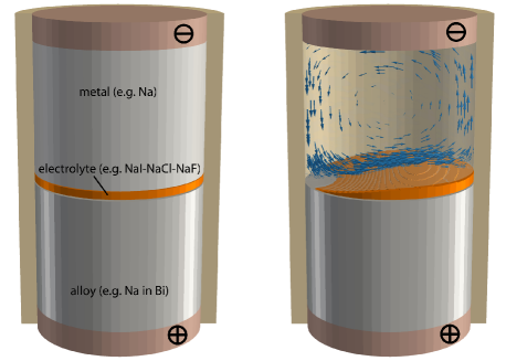
Figure 1: Sketch of a liquid metal battery with typical inventory (left). The electrolyte works as ion conductor and separates the two liquid metals. A movement of the fluid may wipe the electrolyte and lead to an internal short-circuit and thereby a battery failure (right). The TI will induce one or several convection cells in the conducting liquid metal layers.

While small versions of such batteries have already been tested [15], the occurrence of the TI could represent a serious problem for the integrity of the stratification in larger batteries [18]. This is all the more an issue as the highly resistive electrolyte should be chosen as thin as possible in order to maintain a reasonable cell voltage. In [18] we had proposed a simple trick to suppress the TI in liquid metal batteries by just returning the battery current through a bore in the middle. By the resulting change of the radial dependence of $B_{\varphi}(r)$ it is possible to prevent the (ideal) condition (1) for the onset of the TI.

In spite of such attempts to suppress the TI, it is worthwhile to study in detail the flow structure that would arise from it, and the resulting consequences on the stratification of the three layer system. A first step in this direction is the determination of the final velocity field in the saturated state of the TI. The code utilized up to now for the simulation of the liquid metal experiment was well capable of determining the critical current and the growth rates for the onset of the TI [19], but the resulting scale of the velocity in the saturated state was less secure. This has to do with the fact that liquid metals are characterized by a very small magnetic Prandtl number $Pm:=\nu\mu_{0}\sigma\sim 10^{-6}...10^{-5}$. The usual numerical schemes for the simulation of TI, which solve the Navier-Stokes equation for the velocity and the induction equation for the magnetic field, are working typically only for values of $Pm$ down to 10^-2. When applying the code at these much too high $Pm$, and scaling the resulting velocity level by $\nu/R$, one arrives at velocity scales in the order of mm/s. However, an extrapolation over 4 orders of magnitude is somehow risky, and needs definitely a justification by codes that can cope with realistic values of $Pm$.

In this paper, we circumvent the $Pm$ limitations of those codes that rely on the differential equation approach. We do this by replacing the solution of the induction equation for the magnetic field by applying the so-called quasistatic approximation [20]. This approximation means that we skip the explicit time dependence of the magnetic field by computing the electrostatic potential by a Poisson equation, and deriving then the electric current density. However, in contrast to many other applications in which this procedure is sufficient, in our case we cannot avoid to compute the induced magnetic field, too. The reason for that is the existence of an externally applied current in the fluid. Computing the Lorentz force term it turns out that the product of the applied current times the induced field is of the same order as the product of the magnetic field (due to the applied current) times the induced current. Here, we compute the induced current density from the induced magnetic field by means of Biot-Savart’s law. This way we arrive at an integro-differential equation approach, as it had already been used by Meir and Schmidt [21].

In the following, we will describe the mathematical basis of the integro-differential equation approach in the quasistatic approximation. Then we will present the developed numerical model that utilizes the open source CFD library OpenFOAM^® [22], supplemented by an MPI-parallelized implementation of Biot-Savart’s law. We will discuss, in particular, the convergence properties of this numerical scheme when applied to a TI problem in cuboid geometry. Based on this, we will study the effect of a varying geometric aspect ratio on the spatial structure of the TI and on the critical current. We will also discuss the effect of spontaneous chiral symmetry breaking as it was recently discussed by Gellert et al[23] and Bonanno et al[24]. Then, we will apply our model to the cylindrical TI experiment [1], for which we will show a surprising agreement between measured and computed growth rates. The paper closes with a discussion of the results, with an outlook towards more detailed simulations of liquid metal batteries, and with prospects for a larger TI-related experiment.

2 Mathematical Model

The initial point for describing fluid dynamics in a liquid metal is the Navier-Stokes equation (NSE)

$$\dot{\bi v}+\left({\bi v}\cdot\nabla\right){\bi v}=-\frac{\nabla p}{\rho}+\nu\Delta{\bi v}+\frac{\bi f}{\rho},$$ (2)

with ${\bi v}$ denoting the velocity, $p$ the pressure, $\rho$ the density, $\nu$ the kinematic viscosity, and ${\bi f}$ the body force density. For incompressible fluids the continuity equation $\nabla\cdot{\bi v}=0$ has to be taken into account.

The trigger of the TI is the Lorentz force,

$$\bi f=\bi f_{\mathrm{L}}=\bi J\times\bi B,$$ (3)

with $\bi J$ meaning the current density. Note that the magnetic field ${\bi B}$ consists of two parts: the static field $\bi B_{\mathrm{0}}$, generated by the applied current $I$ (or the corresponding current density $\bi J_{\mathrm{0}}$), and the induced magnetic field ${\bi b}$, generated by the motion of the electrically conducing fluid. Although in our problem ${\bi b}$ is rather small, it must not be neglected in the expression for the Lorentz force because it is multiplied with the large current density ${\bi J_{\mathrm{0}}}$.

The usual way to simulate the magnetic field evolution is by solving the induction equation

$$\dot{\bi B}+({\bi v}\cdot\nabla){\bi B} =\left({\bi B}\cdot\nabla\right){\bi v}+\frac{1}{\mu_{0}\sigma}\Delta{\bi B}\;.$$ (4)

The solution of this equation requires suitable boundary conditions for the magnetic field, which can be implemented either by solving a Laplace equation in the exterior of the fluid [25, 26], or by equivalent boundary element methods [27, 28, 29].

In the following, we choose a second option, i.e. we compute the magnetic field using Biot-Savart’s law

$${\bi B}({\bi r})=\frac{\mu_{0}}{4\pi}\int dV^{\prime}\,\frac{{\bi J}({\bi r}^{\prime})\times({\bi r}-{\bi r}^{\prime})}{\left|{\bi r}-{\bi r}^{\prime}\right|^{3}},$$ (5)

which is the inversion of Ampère’s law $\nabla\times\bi B=\mu_{0}\bi J$. Here ${\bi r}$ means the point coordinate where $\bi B$ has to be computed, and ${\bi r}^{\prime}$ is the integration coordinate, which runs through the whole domain where ${\bi J}$ exists.

This way, the problem is shifted from the determination of the magnetic field $\bi B$ to the determination of the current density $\bi J$. The approach to use Biot-Savart’s law was already proposed and utilized by Meir et al[21], and will be adopted to our case.

The flow chart of the numerical model is shown in figure 2. Assuming the current $I$ through our cylindrical vessel as given (e.g. the battery charging current), we compute the corresponding current density $\bi J_{\mathrm{0}}$, and the associated static magnetic field $\bi B_{\mathrm{0}}$. For an infinitely long vertical cylinder we would obtain

$${\bi B_{\mathrm{0}}}(x,y)=\frac{\mu_{0}J_{0}}{2}\left(y\bi{e_{x}}-x\bi{e_{y}}\right),$$ (6)

in Cartesian coordinates $x,y,z$. For real geometries with external leads to the system, $\bi B_{\mathrm{0}}$ could still be be computed by Biot-Savart’s law.

In the main loop of our numerical scheme, the Navier-Stokes equation (2) is solved firstly, followed by a velocity corrector step to ensure continuity ($\nabla\bi\cdot\,\bi v=0$). Then we have to find the electric current density. Presupposing the magnetic Reynolds number $Rm=\mu_{0}\sigma Rv$ on the basis of the the TI-triggered velocity scale $v$ to be small, we can invoke the quasistatic approximation [20]. This means that we express the electric field by the gradient of an electrostatic potential, ${\bi E}=-\nabla\Phi$. Applying the divergence operator to Ohm’s law in moving conductors, ${\bi J}=\sigma(-\nabla\Phi+{\bi v}\times{\bi B})$, and demanding charge conservation, $\nabla\cdot{\bi J}=0$, we arrive at the Poisson equation

$$\Delta\varphi=\nabla\cdot\left({\bi v}\times{\bi B}\right)$$ (7)

for the perturbed electric potential $\varphi=\Phi-J_{0}z/\sigma$, where $z$ is the coordinate along the battery axis pointing into the direction of the applied potential difference. By subtracting the electric potential caused by the battery charging current $I$ we can easily set the boundary conditions at the electrodes to $\varphi=0$. Since no current is allowed to flow through the insulating rim of the cylindrical vessel, we assume here $\nabla\varphi=0$.

Having derived the potential in the fluid by solving the Poisson equation, we easily recover the current density induced by the fluid motion as

$${\bi j}=\sigma\left(-\nabla\varphi+{\bi v}\times{\bi B}\right)$$ (8)

and then the induced magnetic field by using Biot-Savart’s law (5). The total current density is

$${\bi J}=\bi j-J_{0}\bi e_{z}.$$ (9)

In a last step, the Lorentz force, to be implemented into the Navier-Stokes equation, is calculated according to

$$\bi f_{\mathrm{L}}=\bi J\times{\bi B}=\left(\sigma\left(-\nabla\varphi+{\bi v}\times\left(\bi B_{\mathrm{0}}+{\bi b}\right)\right)-J_{0}\bi e_{z}\right)\times\left(\bi B_{\mathrm{0}}+{\bi b}\right).$$ (10)

It should be noticed again that the (small) induced magnetic field $\bi b$ cannot be omitted here, since its product with the (large) impressed current $\bi J_{0}$ is of the same order as the product of the (small) induced current $\bi j$ with the (large) magnetic field $\bi B_{0}$.

Assuming an implementation of this scheme on a certain grid, one has to ask for the allowed time steps to keep the time evolution of the system stable. For this it is important to consider not only the Courant number based on the hydrodynamic velocity $v$, but also the Alfvén-Courant number based on the Alfvén velocity $v_{A}=B/(\mu_{0}\rho)^{1/2}$. The influence of the Alfvén-Courant number on the accuracy of the simulations is discussed in the following section.

Figure 2: Flow chart of the simulation model.

3 Numerical scheme and convergence

In this section we will examine the numerical scheme with respect to its convergence and error characteristics. We will both study variations of the grid spacing as well as of the time steps. We will further consider the case that different grid spacings and time steps are used for the Navier-Stokes equation and for the Biot-Savart law.

In order to utilize the convenience of orthogonal cells for grid refinement, a cuboid with the dimensions of $96\times 96\times$120\text{\,}\mathrm{m}\mathrm{m}^{3}$$ is used as a reference geometry, see figure 3.

Anticipating the later simulation of the recent TI experiment [1], we will start to work here with the real material parameters of GaInSn: electric conductivity $\sigma=$3.29\text{\cdot}{10}^{6}\text{\,}\mathrm{S}\text{{}\cdot{}}{\mathrm{m}}^{-1}$$, density $\rho=$6403\text{\,}\mathrm{k}\mathrm{g}\mathrm{/}\mathrm{m}^{3}$$, kinematic viscosity $\eta=$3.4\text{\cdot}{10}^{-7}\text{\,}\mathrm{m}^{2}\mathrm{/}\mathrm{s}$$. The applied current is set to $10\text{\,}\mathrm{kA}$.

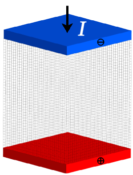
Figure 3: Geometric setting for the simulation of the TI in cuboid geometry. The electric current is assumed to be impressed by infinitely long electrodes. The Navier-Stokes equation, enhanced by the Poisson equation and the Biot-Savart law, is solved in the gridded volume between the electrodes.

For this case, figure 4 shows a typical evolution of the TI in time, comprising an initial phase were the eigenfield of the TI develops, followed by a long period (over $\sim$ $600\text{\,}\mathrm{s}$) in which this eigenfield grows exponentially, and a final phase in which the TI saturates at a certain velocity level.

In the following we will compare the growth rates, as they can be read off during the exponential growth phase for different grid spacings and time steps, with respect to their relative errors which are derived by dividing the absolute error by the difference of the TI growth rates at $10\text{\,}\mathrm{kA}$ and $0\text{\,}\mathrm{kA}$.

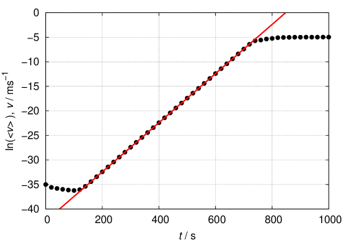
Figure 4: The typical flow development of the TI is characterized by an initial phase, an exponential growth phase, and a final saturation phase (black dotted line). The growth rate corresponds to the slope of the red line.

3.1 Grid refinement

We start by exploring the effects of different grid sizes of the cubic cells with an edge length between $1\text{\,}\mathrm{mm}$ and $8\text{\,}\mathrm{mm}$. Using the Finite-Volume-Method (FVM) of OpenFOAM^® for the simulation, the values from the cell centres have to be interpolated to the cell faces in order to ensure continuity. For this interpolation we employ two different methods, a linear one and a cubic one, and compare the results in figure 5. As expected, the cubic interpolation provides better results, i.e. the growth rates are typically higher. While it would be numerically very demanding to go below a cell size of $1\text{\,}\mathrm{m}\mathrm{m}$, we expect the difference between cubic and linear interpolation to be zero in the limit of vanishing cell size. With that assumption we do a Richardson extrapolation to obtain the ”true” growth rate of the TI. Taking this value as reference, the relative error of the growth rates is then calculated in dependence on the grid cell size (figure 6).

Since the solution of the Biot-Savart law is numerically very costly, we have additionally checked the possibility to speed up this part of the simulation. While the two lines in figure 5 result from computations in which the Navier-Stokes equation and the Biot-Savart law are implemented on the same grid, the green circles and the liqht blue squares correspond to cases in which the Biot-Savart law is realized on coarser grids. In contrast to the ${\bi b}$-calculation with cells of $8\text{\,}\mathrm{mm}$ edge length, which does not give good results (see figure 5), a grid cell size of $6\text{\,}\mathrm{mm}$ already seems to be sufficient. Solving the Navier-Stokes equation on a $3\text{\,}\mathrm{mm}$ grid, and computing Biot-Savart’s law on a $6\text{\,}\mathrm{mm}$ grid, provides almost the same results as doing both on a $3\text{\,}\mathrm{mm}$ grid. This is numerically very convenient because Biot-Savart’s law needs the square of cell numbers as operations whenever carried out, i.e. a coarse grid makes simulation much faster. The resulting slightly lower growth rates when working with two meshes appear due to the inter-grid mapping. The interpolation flattens the ${\bi b}$-field a little bit which reduces the growth rate – but the difference is very small.

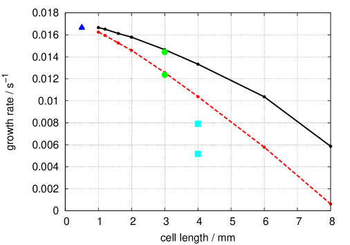
Figure 5: Influence of the grid cell size on the growth rate. Simulation is carried out for linear cell-face interpolation (red dashed line) as well as cubic one (black line). Computing Biot-Savart’s law with $8\text{\,}\mathrm{mm}$ cells does not give good results (${\color[rgb]{0,1,1}\blacksquare}$), while a $6\text{\,}\mathrm{mm}$ grid is sufficient (${\color[rgb]{0,1,0}\bullet}$). This technique allows an additional refinement of the initial mesh, i.e. to solve the NSE on a $0.5\text{\,}\mathrm{mm}$ grid (${\color[rgb]{0,0,1}\blacktriangle}$).

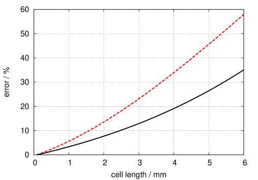
Figure 6: Influence of the grid cell size on the error of the growth rate. The maximal growth rate at $0\text{\,}\mathrm{mm}$ was extrapolated from $1\text{\,}\mathrm{mm}$ cells and used as reference. The black line stands for cubic cell-face interpolation, the red dotted one for linear interpolation.

3.2 Alfvén-Courant number and time steps

As usually, during the time integration of the NSE we have to fulfill the Courant-Friedrichs-Lewy (CFL) condition for the time step. In our special problem, however, information is not only transferred by the flow velocity, but also electromagnetically with the Alfvén velocity $v_{A}=B/(\mu_{0}\rho)^{1/2}$. We consider this by introducing an “Alfvén-Courant number” and compute the maximum time step on that basis. Due to the high currents at which TI is expected to set in, and the consequently high magnetic field $B_{0}$, this time step has to be very short in spite of the low fluid velocities. Fortunately, it turns out that choosing the Alfvén-Courant number larger than one does not lead to a completely unstable system, as it would be expected for a purely differential equation system. Evidently, the mixed integro-differential equation approach makes the system somewhat more “benign” and less vulnerable to violations of the CFL condition. Of course, the error increases significantly with increasing Alfvén-Courant number as shown in figure 7.

Figure 7: Influence of the Alfvén-Courant number on the error of the growth rate. The Alfvén-Courant number is one, if a particle, moving with Alfvén velocity, passes exactly one grid cell in one time step.

Besides calculating the magnetic field ${\bi b}$ on a coarser grid than the velocity field, we have also tested to compute it only at every n^th timestep. Figure 8 shows that it is well possible to compute the Biot-Savart integrals only every 100^th time step. The benefit in computation time is especially high when solving the NSE and Biot-Savart’s law on the same grid, as the latter one takes usually more than 100 times longer than solving all other equations.

Figure 8: Error of the growth rate of the TI depending on how often the induced magnetic field $\bi b$ is calculated. As the TI is growing slowly and therefore $\bi b$ changes slowly, the simulation can be accelerated by doing Biot-Savart not every time step.

4 Results for cuboid geometry

In this section we will focus on the characteristic eigenmode structure of the TI, on the typical velocities in the saturated regime, and on the critical currents in dependence on various geometry parameters. The simulation are done for a cuboid volume with a base area of $96\times 96$ mm², but with varying heights.

4.1 Shape, alignment, and chiral symmetry breaking

Basically, the TI appears in form of convection cells that are vertically stacked one over another (see figure 9). The fluid in one cell rotates around some horizontal axis, and the sense of rotation is changing from one cell to the neighboring one. Referring, for the moment, to cylindrical geometry, this cell structure represents a non-axisymmetric flow structure, with an azimuthal wavenumber $m=\pm 1$. Since the present simulations are carried out for cuboid geometry, one could imagine, e.g., a preferred alignment of the convection cells with the diagonal of the base area. However, this is generally not the case. In fact, the alignment of the cells depends strongly on the chosen initial conditions. Assuming a small perturbation in the $x$-direction, the TI will arise around the $y$-axis (figure 9). For arbitrary initial velocity, the TI will develop around a random axis.

Most interestingly, a transient helical shape of the TI may result under certain initial conditions (see figure 9, right). This was observed, e.g., with an initial velocity in $z$-direction and in particular when the height of the simulated geometry did not match an integer multiple of the wave length of the TI. The helical perturbation may develop if, e.g., two convection cells arise simultaneously, but with azimuthal twisted rotation axes. The growth rates of the non-helical and the helical TI state were found to be very similar. Figure 10 shows the velocity and the normalized mean value of the helicity $H={\bi v}\cdot(\nabla\times{\bi v})$ of a non-helical (blue) and of a helical (red) state for a $96\times 96\times 360$ mm³ geometry ($h=3.1\lambda$). Reaching a certain velocity level in the saturated regime, the helicity of the helical state reduces significantly and goes finally to zero. Approximetaly at the same time (at $\sim$2500 s) the saturated state of the formerly non-helical state acquires also some helicity, which goes finally to zero, too. The ultimate convection cells of the two states are not equal (compare figure 9 left and right), and seem to depend on the different initial conditions of the velocity.

This transient appearance of helical TI structures is quite remarkable, since it corresponds to the spontaneous chiral symmetry breaking which was recently observed by Gellert et al[23] and discussed in detail by Bonanno et al[24]. Here we can only evidence its occurrence, while a more comprehensive study of this effect has to be left for future studies.

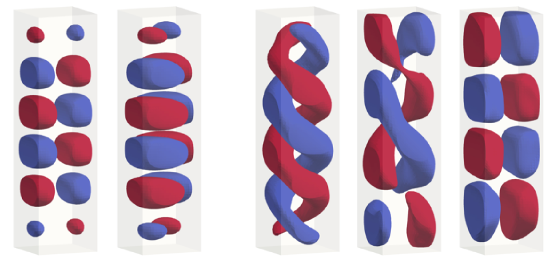
Figure 9: Iso-surface plots of the magnetic field $b_{z}$ for a cuboid of $h=$360\text{\,}\mathrm{mm}$$. Depending on the initial velocity conditions, the convection cells of the TI align to an arbitrary direction (left: orthogonal, second: diagonal to base cube). Due to a helical perturbation, a helical TI may grow (3. panel, $t=$2300\text{\,}\mathrm{s}$$), but almost disappears later (4. panel $t=$2400\text{\,}\mathrm{s}$$, right $t=$2800\text{\,}\mathrm{s}$$). The corresponding time graph is shown in figure 10.

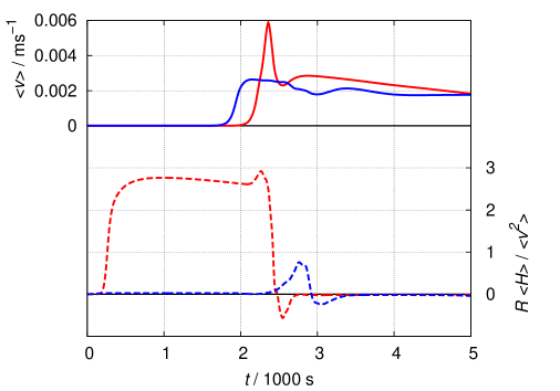
Figure 10: Temporal evolution of the mean velocity (continuous lines in the upper part) and of the corresponding normalized helicity (dotted lines in the lower part), with $H=\bi v\cdot(\nabla\times\bi v)$ and $R$ as the half side length of the base square. The height of the cuboid is $360\text{\,}\mathrm{mm}$, the applied current $10\text{\,}\mathrm{kA}$. The blue lines correspond to an initial velocity along the diagonal of the base cube, while the red plots result from an initial velocity in $z$ direction.

4.2 Saturation levels of the TI

To investigate the saturation level of the TI we have carried out simulations using different currents for a cuboid geometry of 96$\times$96$\times$120 mm³ and a grid cell length of $3\text{\,}\mathrm{mm}$. When the critical current for the onset of the TI is exceeded, any small disturbance can initiate the instability which then needs some time to establish its eigenmode. Thereafter, this eigenmode grows exponentially, see figure 11. For currents only slightly above the critical one, the instability grows very slowly. In such a case, it may take tens of minutes until the TI reaches its saturated final state. Figure 12 shows the dependence of the final velocities on the applied current. We see that the maximum velocities grow from a few mm/s close to the critical current, to nearly 14 cm/s at $50\text{\,}\mathrm{kA}$. Velocities on this scale would clearly be problematic for the stability of the layer stratification in liquid metal batteries.

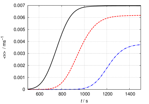
Figure 11: Development of the mean velocities of the TI in function of time for different applied currents: $I=$14\text{\,}\mathrm{kA}$$ (blue line), $I=$16\text{\,}\mathrm{kA}$$ (red line) and $I=$18\text{\,}\mathrm{kA}$$ (black line).

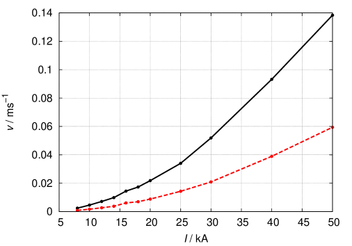
Figure 12: Dependence of velocity of the TI on the applied current $I$. The black line stands for maximum velocities, the red dashed line for averaged velocities.

4.3 Critical current in dependence on the aspect ratio

To investigate the dependence of the critical current on the aspect ratio of the fluid volume we consider a cuboid with a base area of $96\times$96\text{\,}\mathrm{m}\mathrm{m}^{2}$$ which is changed in height from 24 to $480\text{\,}\mathrm{mm}$.

As a first estimate for the critical wavelength of the TI we can take the value for an infinitely long cylinder of radius $R$,

$$\lambda=2\pi R/k,$$ (11)

for which the critical wavenumber $k$ is known to be 2.47 [19]. Embedding this cylinder in the cuboid to be considered here, the resulting wave length would be $\lambda=$122\text{\,}\mathrm{mm}$$. To obtain the corresponding true spatial wave length for the cuboid geometry, the TI is simulated for a very long cuboid with a height of $1040\text{\,}\mathrm{mm}$. For this case we obtain $\lambda=$115\text{\,}\mathrm{mm}$$, a value quite close to the corresponding value of the infinitely long cylinder.

Figure 13 shows now the critical currents as a function of height. In the limit of very tall cuboids, the critical current converges to a value of approximately $3\text{\,}\mathrm{kA}$ which is also quite close to the value $2.7\text{\,}\mathrm{kA}$ for the infinite long cylinder [19]. Shortening the cuboid, a first plateau of the critical current is observed at a height corresponding to the TI wave length of $115\text{\,}\mathrm{mm}$. Decreasing the height further, a sharp increase of the critical current is observed, which flattens again to a second plateau when the height comes close to the half wave length ($57.5\text{\,}\mathrm{mm}$). Shortening the cuboid still further, the critical currents rise extremely steep. With regard to liquid metal batteries this would mean that very flat cells will not be affected by the Tayler instability.

For those heights which are below the half wavelength of the TI ($h<\lambda/2$), there is only one convection cell, for slightly taller vessels a second one appears (see figure 13, left). In general, the number of convection cells adapts to the height, and the cell size acquires a maximum if the height is a multiple of the wavelength. If $h$ exceeds $1.5\lambda$, a third cell may appear – but only in case of a helical TI. In case of non-helical TI an even number of convection cells seems to be more stable. Usually, the new convection cells appear at the top and/or bottom. If the height is slightly below an integer multiple of the characteristic wave length, the upper and lower convection cell will appear somehow ”compressed” in comparison to the more central ones (figure 13, right).

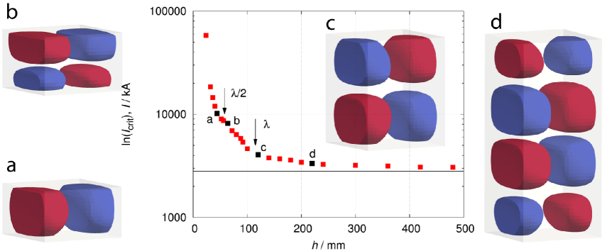
Figure 13: Dependence of the critical current for the onset of the TI on the height of a cuboid of $96\times 96\times h$ mm³. If the height of the vessel drops below the wave length of the TI, the critical current increases steeply. The black line marks the critical current for the infinite cylinder. The isosurface plots show the induced magnetic field ${b_{z}}$ for four selected heights $h$, indicated by the black cubes in the graph. Below one half wave length ($h<\lambda/2$), only one convection cell is present (a). Slightly above $h=\lambda/2$, there are two cells (b). Panel c shows the case when $h=\lambda$. For $h=1.9\lambda$ (d), we observe four cells, the top and bottom ones appearing somewhat smaller.

5 Validation of experimental results

In a recent paper [1], we had evidenced the occurrence of the TI in a liquid metal experiment. A cylinder, made of polyoxylmethylene ($d=$100\text{\,}\mathrm{mm}$$, $h=$750\text{\,}\mathrm{mm}$$) was filled with the eutectic GaInSn, being liquid at room temperature. A current of up to 8 kA was injected into the liquid metal through two massive copper electrodes at the top and bottom of the cylinder. In order to avoid any inhomogeneities of the electric current at the interface between Cu and GaInSn, we restrained from inserting ultrasonic transducers for the direct measurement of the velocity perturbations, and relied exclusively on external measurements of the induced magnetic field. The vertical component $b_{z}$ was measured at 11 positions along the vertical axis of the device. With this set-up we were able to identify the growth rates of the short-wavelength perturbations due to the TI, before those gave way to longer wavelength structure that we attributed to the thermal wind resulting from Joule heating in the GaInSn.

For this cylindrical geometry, we simulate the TI and compare the results with the available experimental data. The cylindrical fluid volume is meshed with a grid cell size of about $3\times 3\times 3$ mm³. As the electrodes are relatively thick and are elongated by long power supply leads, we assume $\bi B_{\mathrm{0}}$ to be constant over the height of the cylinder.

For an assumed current of $10\text{\,}\mathrm{kA}$, the resulting convection cells of the TI are illustrated in figure 14. It should be noticed that the number and shape of these convection cells is quite independent on the initial conditions.

The experimental growth rates are compared with the numerical ones in figure 15. Simulations for the infinitely long cylinder [19] provide the maximum possible growth rates. As we do simulation for the real, i.e. finite cylinder, the resulting growth rates lie slightly below these values, but correspond nicely with the experimental data.

For our geometry the theoretical wave length is $\lambda=$127\text{\,}\mathrm{mm}$$ [19]. This value matches fairly well the wave length obtained by our finite length simulation ($121\text{\,}\mathrm{mm}$), as inferred from figure 16.

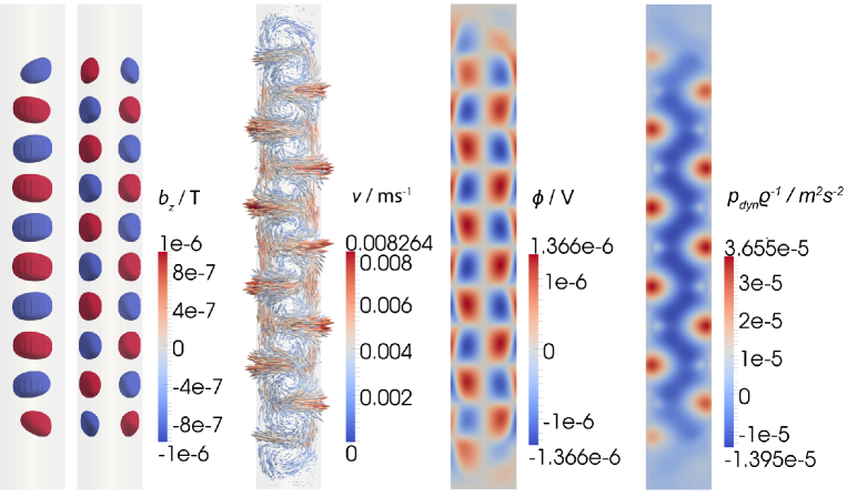
Figure 14: Iso-shapes for $b_{z}$ (left), velocity field (second panel), electric potential (third panel) and dynamic pressure (right) of the saturated Tayler instability in a cylinder filled with GaInSn. The applied current is $10\text{\,}\mathrm{kA}$. The magnetic field is shown in $x$ and $y$ direction, all other figures only in $x$.

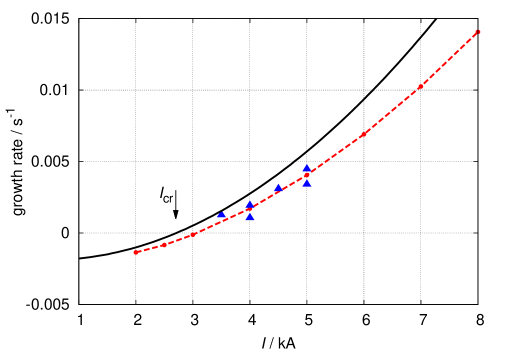
Figure 15: Growth rates of the Tayler instability in a cylinder filled with GaInSn. The black line marks the maximal possible growth rates for the infinite cylinder [19]. Our simulation (red dashed line) fits well the experimental data (blue triangles) [1].

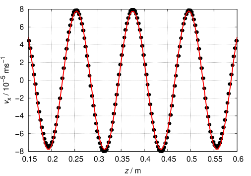
Figure 16: Velocities of the TI in $x$-direction along the $z$-axis in the central part. Values are taken at maximal growth rate, i.e. shortly before reaching saturation (black dotted line). The red fit allows to determine the spatial wavelength of $\lambda=$121\text{\,}\mathrm{mm}$$.

6 Conclusion and outlook

On the basis of an integro-differential equation approach we have developed a numerical tool that is particularly suited for investigations of current driven magnetohydrodynamic instabilities in liquid metals. Employing the quasistatic approximation, the solution of the induction equation for the magnetic field was substituted by solving a Poisson equation for the induced current density, from which the magnetic field is computed via Biot-Savart’s law. This procedure allows to deal with instabilities in conducting fluids characterized by very small magnetic Prandtl numbers.

After examining the convergence properties of this numerical scheme, we have simulated the TI in different geometries, including cuboids and cylinders. For the cuboid it was shown in detail how the critical current increases with decreasing aspect ratio, exhibiting two remarkable plateaus at those heights that correspond to one or a half wavelength of the TI mode, respectively. This curve may be directly used for defining a maximum aspect ratio of liquid metal batteries at a given charging current. Depending on the initial conditions our simulations have also shown the transient appearance of helical structures, i.e. the occurrence of chiral symmetry breaking.

For cylindrical geometry, we have numerically reproduced the growth rates of the TI that had been measured in a recent liquid metal experiment.

A main result of our simulations is that the saturation level of the TI induced velocity for typical electrical currents are in the order of mm/s until cm/s. This is quite consistent with a formal scaling, by $\nu/R$, of the velocity levels as obtained at much larger magnetic Prandtl numbers [30]. While this good correspondence confirms the interaction parameter $\mathit{Ha}^{2}/Re$ to be the governing parameter for the saturation over a wide range of magnetic Prandtl numbers, it makes the physical interpretation of the saturation mechanism a bit more difficult. Actually, for $Pm$ close to one, Gellert et al[30] had identified a very plausible saturation mechanism in terms of a radially dependent increase of the TI triggered turbulent resistivity ($\beta$ effect) that modifies the radial current distribution in such a way as to make the magnetic field distribution just marginally stable. Evidently, this nice picture does not apply any more for small $Pm$, as considered here, since the arising velocity perturbation are much too weak for producing any noticeable turbulent resistivity. In this respect, a simple picture for understanding the saturation of TI at low $Pm$ remains elusive.

In a next step we plan to include into the numerical model the effects of thermal convection resulting from the Joule heating due to the strong current, which has turned out important in the experiment. We also develop a multiphase solver which will allow us to simulate three-layer liquid metal batteries in detail.

On the experimental side, in the framework of the DRESDYN project [31] we plan to set-up a large scale liquid sodium experiment for the combined investigation of the magneto-rotational instability, as recently investigated [32], and the TI.

References

References

- [1] Seilmayer M, Stefani F, Gundrum T, Weier T, Gerbeth G, Gellert M and Rüdiger G 2012 Phys. Rev. Letters 108 244501
- [2] Tayler R J 1960 Rev. Mod. Phys. 32 907 – 913
- [3] Bergerson W F, Forest C B, Fiksel G, Hannum D A, Kendrick R, Sarff J S and Stambler S 2006 Phys. Rev. Lett. 96 015004
- [4] Vandakurov Y V 1972 Astron. Zh+. 49 324 – 333
- [5] Tayler R J 1973 Mon. Not. R. astr. Soc. 161 365 – 380
- [6] Spruit H C 2002 Astron. Astrophys. 381 923 – 932
- [7] Zahn J P, Brun A S and Mathis S 2007 Astron. Astrophys. 474 145 – 154
- [8] Suijs M P L, Langer N, Poelarends A J, Yoon S C, Heger A and Herwig F 2008 Astron. Astrophys. 481 L87 – L90
- [9] Yoon S C, Dierks A and Langer N 2012 Astron. Astrophys. 542 A113
- [10] Moll R, Spruit H C and Obergaulinger M 2008 Astron. Astrophys. 492 621 – 630
- [11] Spies G O 1988 Plasma Phys. Control. Fusion 30 1025 – 1037
- [12] Cochran F L and Robson A E 1993 Phys. Fluids B 5 2905 – 2908
- [13] Rüdiger G, Schultz M and Gellert M 2011 Astron. Nachr. 10 1 – 7
- [14] Huggins R E 2010 Energy Storage (Springer Sciene+Business Media)
- [15] Bradwell D J, Kim H, Sirk A H C and Sadoway D R 2012 J. Am. Chem. Soc. 134 1895 – 1897
- [16] Weaver R D, Smith S W and Willmann N L 1962 J. Electrochem. Soc. 109 653 – 657
- [17] Cairns E J and Shimotake H 1969 Science 164 1347 –1355
- [18] Stefani F, Weier T, Gundrum T and Gerbeth G 2011 Energ. Convers. Manage. 52 2982 – 2986
- [19] Rüdiger G, Gellert M, Schultz M, Strassmeier K G, Stefani F, Gundrum T, Seilmayer M and Gerbeth G 2012 Astrophys. J. 755 181
- [20] Davidson P A 2001 An Introduction to Magnetohydrodynamics (Cambridge University Press)
- [21] Meir A J, Schmidt P G, Bakhtiyarov S I and Overfelt R A 2004 J. Appl. Mech. 71 786 – 795
- [22] OpenFOAM Foundation 2012 http://www.openfoam.org/
- [23] Gellert M, Rüdiger G and Hollerbach R 2011 Mon. Not. R. Astron. Soc. 414 2696 – 2701
- [24] Bonanno A, Brandenburg A, Del Sordo F and Mitra D 2012 Phys. Rev. E 86 016313
- [25] Stefani F, Gerbeth G and Gailitis A 1999 Velocity profile optimization for the Riga dynamo experiment Transfer Phenomena in Magnetohydrodynamics and Electrocinducting flows ed Alemany A, Marty P and Thibault J P (Kluwer Dordrecht) pp 31 – 44
- [26] Guermond J L, Laguerre R, Léorat J and Nore C 2007 J. Comput. Phys. 221 349 – 369
- [27] Stefani F, Gerbeth G and Rädler K H 2000 Astron. Nachr. 321 65 – 73
- [28] Iskakov A, Descombes S and Dormy E 2004 J. Comput. Phys. 197 540 – 554
- [29] Giesecke A, Stefani F and Gerbeth G 2008 Magnetohydrodynamics 44 237 – 252
- [30] Gellert M and Rüdiger G 2009 Phys. Rev. E 80 046314
- [31] Stefani F, Eckert S, Gerbeth G, Giesecke A, Gundrum T, Steglich C, Weier T and Wustmann B 2012 Magnetohydrodynamics 48 103 – 113
- [32] Stefani F, Gerbeth G, Gundrum T, Hollerbach R, Priede J, Rüdiger G and Szklarski J 2009 Phys. Rev. E 80 066303