Single-Pass GPU-Raycasting for
Structured Adaptive Mesh Refinement Data

Abstract

Structured Adaptive Mesh Refinement (SAMR) is a popular numerical technique to study processes with high spatial and temporal dynamic range. It reduces computational requirements by adapting the lattice on which the underlying differential equations are solved to most efficiently represent the solution. Particularly in astrophysics and cosmology such simulations now can capture spatial scales ten orders of magnitude apart and more. The irregular locations and extensions of the refined regions in the SAMR scheme and the fact that different resolution levels partially overlap, poses a challenge for GPU-based direct volume rendering methods. kD-trees have proven to be advantageous to subdivide the data domain into non-overlapping blocks of equally sized cells, optimal for the texture units of current graphics hardware, but previous GPU-supported raycasting approaches for SAMR data using this data structure required a separate rendering pass for each node, preventing the application of many advanced lighting schemes that require simultaneous access to more than one block of cells. In this paper we present the first single-pass GPU-raycasting algorithm for SAMR data that is based on a kD-tree. The tree is efficiently encoded by a set of 3D-textures, which allows to adaptively sample complete rays entirely on the GPU without any CPU interaction. We discuss two different data storage strategies to access the grid data on the GPU and apply them to several datasets to prove the benefits of the proposed method.

1 INTRODUCTION

Multi-scale phenomena are common in many areas of research, in particular astrophysics and cosmology, fluid dynamics, and mechanical engineering. An example is the formation of the first stellar objects in the Universe, involving spatial scales that range from several 10,000 light years, representing the overall dynamics of the proto-galaxies, down to the star forming regions in the order of a few light hours across [1, 2]. Tackling such processes numerically is a challenging task, and naive approaches using constant resolution fail due to their exorbitant computational requirements. Hence adaptive techniques are crucial for this type of problems, as they allow to locally adjust the spatio-temporal resolution to the features of the particular system. A popular adaptive approach for numerically solving partial differential equations is Structured Adaptive Mesh Refinement (SAMR) [3]. It combines the simplicity of structured grids with the benefits of local refinement by recursively overlaying regions of the computational domain with patches of structured grids of increasing resolution.

Applying standard visualization techniques to AMR datasets has always been challenging, partly due to the arbitrary extension and placement of the subgrid patches, partly because of their sheer numbers. This holds in particular for GPU-based volume rendering approaches, which leverage the capabilities of texturing units of current graphics hardware architectures. These operate most efficiently on regular grids and therefore a partitioning of the computational domain covered by the SAMR grids into non-overlapping blocks of cells with the same resolution is crucial for good performance. Adaptive kD-tree have been proven to be particularly suitable for this tasks [4, 5, 6], but previous GPU-based methods required a single rendering pass for each of the resulting blocks, which inhibits the direct application of many advanced shading and lighting effects that need to simultaneously access data from more than one subgrid patch or require non-standard blending equations.

In this paper we present a single-pass GPU-raycasting approach for AMR data. It is based on an efficient kD-tree partition of the domain that minimizes the number of generated nodes and can directly be applied also to non-nested subgrids, which refine regions of more than one coarse “parent” grid patch. We propose an efficient encoding of the resulting tree using a set of 3D-textures, enabling the traversal of the tree and an adaptive sampling of the data on the GPU, on a per-pixel basis in the fragment shader, without any CPU interaction. We further discuss two different approaches to store the data associated with the AMR grid patches: one using a packing scheme to organize the patches in a larger memory pool texture, the other employing NVIDIA’s Bindless Texture extension [7] for the OpenGL-API.

The remainder of this paper is organized as follows. In Section 2 we discuss related work. We review the AMR scheme in Section 3 and describe the new kD-tree generation strategy and its encoding on the GPU in Section 4. The GPU-data access scheme as well as the rendering algorithm will be discussed in Section 5. We end with results and conclusions in Section 6 and 7.

2 RELATED WORK

To the best of our knowledge the first CPU-based volume rendering method for AMR data was proposed by Max [8]. It employed a back-to-front cell-sorting and cell-projection scheme. Later the dual-mesh approach [9], for higher order interpolation of “cell-centered” AMR data without resampling, has been extended for more general subgrid configurations and was used for a direct volume rendering approach [10]. Further several parallel CPU-based volume rendering methods for cluster architectures data have been presented [11, 12].

The first GPU-supported volume rendering approach for AMR data was presented by Weber et al. [6]. The authors applied their dual-mesh-“stitching” scheme to implement a hardware-supported cell-projection algorithm rendering the faces of the resulting cells as semi-transparent triangles. Kaehler et al. presented a 3D-texture-based volume rendering approach for large, sparse datasets, that clusters non-transparent voxels into axis-aligned blocks and encodes these as leaf nodes of AMR data structures. [13] They also described a multi-resolution texture-based volume rendering algorithm for AMR data [4]. Park et al. [14] presented a hierarchical splatting approach for AMR data. Kelley et al. [5] describe a framework for interactive, parallel volume rendering of remote AMR data, that distributes subtrees of the AMR hierarchy on individual processors and composes the images on a local rendering client.

With the advent of programmable graphics hardware that supports flexible shader programs, it became feasible to perform the ray integration on a per-pixel basis at interactive frame rates [15, 16, 17]. In the latter approach the data is converted to a 3D texture and a fragment shader is executed for each pixel that is covered by the projected bounding box of the data volume. The ray is parameterized in texture coordinates and the ray-integral is computed in the fragment shader. GPU-raycasting is particularly attractive for adaptive grids, as it does not suffer from the rendering artifacts inherent to slice-based methods, which can lead to visible artifacts at the interfaces between different resolution levels. GPU-raycasting has been extended to SAMR data, using a kD-tree that is traversed on the CPU and rendered node-by-node in separate rendering passes [18].

All previous approaches for single-pass multi-resolution GPU-raycasting were based on regular data structures, such as octrees or other partition strategies using regularly shaped nodes [19, 20, 21, 22]. In principle also AMR data structures can be partitioned in blocks of cells from the same resolution level using octrees. However, the resulting tree is usually inefficient, in particular if higher order interpolation is desired, because of the large number of resulting nodes [13]. In contrast kD-trees allow to minimize the number of nodes by adaptively choosing the position of the spatial subdivision planes and have been successfully applied to CPU-, and GPU-based volume rendering of AMR data [4, 5, 6, 23]. In this paper we present the first single-pass GPU-raycasting approach for AMR data based on a kD-partition of the data domain.

3 STRUCTURED ADAPTIVE MESH REFINEMENT

In the Adaptive Mesh Refinement (AMR) [3] approach the computational domain is covered by a set of coarse, structured subgrids.The configuration of this set of coarse grids is usually fixed over time. In a first step the solution of the (partial differential) equations is computed on these coarse grids and local error estimators are utilized to detect cells that require higher resolution. These cells are clustered into a set of rectangular grid patches, usually called subgrids, which do not replace, but rather overlap the corresponding regions of the coarse base grids.

(a)

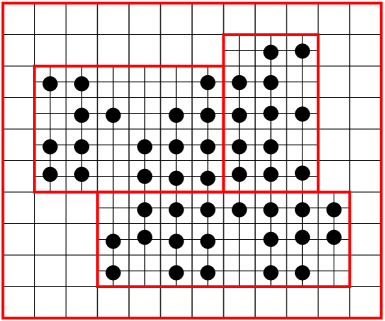
(b)

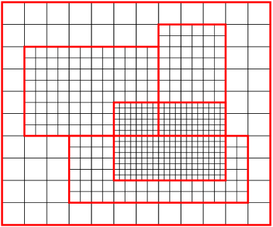
(c)

Figure 1: Refinement process for AMR schemes: Cells that require refinement are determined using local error criteria (a) and clustered into separate subgrids (b), which cover the region at higher resolution. This process is recursively continued (c) until each region has sufficient resolution.

The equations are solved on these higher resolved subgrids, and the refinement procedure recursively continues until all cells have sufficient resolution, giving rise to a hierarchy of nested refinement levels, as shown in Figure 1. A major advantage of AMR is that each subgrid can be viewed as a separate, independent structured grid with its separate storage space. This allows to process subgrids almost independently, and thus it is well-suited for parallel processing. A popular variant of this general approach is Structured Adaptive Mesh Refinement (SAMR) [24], where in contrast to the original scheme, the subgrids are aligned with the major axes of the coordinate system. In the following we will restrict the discussion to SAMR and just refer to it as AMR. In the remainder of this section we will briefly introduce some notations that are used in this paper.

Let ${\bf h}^{0}:=(h^{0}_{0},h^{0}_{1},h^{0}_{2})$ denote the mesh spacing of the coarsest grids. The mesh spacings of the finer grids are recursively defined by ${\bf h}^{l}:=(h^{l-1}_{0}/r,h^{l-1}_{1}/r,h^{l-1}_{2}/r)$ for $l>0$, where the positive integer $r$ denotes the so-called refinement factor and $l$ numbers the refinement level, starting with $0$ for the coarsest level. In principle the refinement factor can differ for each direction and each level, but in order to simplify the notation we assume that it is constant. In the AMR approach, each refined cell is overlaid by a set of $r^{3}$ cells of the next level of refinement. In the original AMR scheme [24] each refinement level was enclosed by at least one layer of cells from the next coarser level of resolution, such that adjacent cells differ by at most one level. This constraint was later relaxed [25, 26]. In the following we will call the set of coarsest subgrids the root level and denote the $m$-th subgrid of the refinement level $l$ by $\Gamma^{l}_{m}$, see Figure 2.

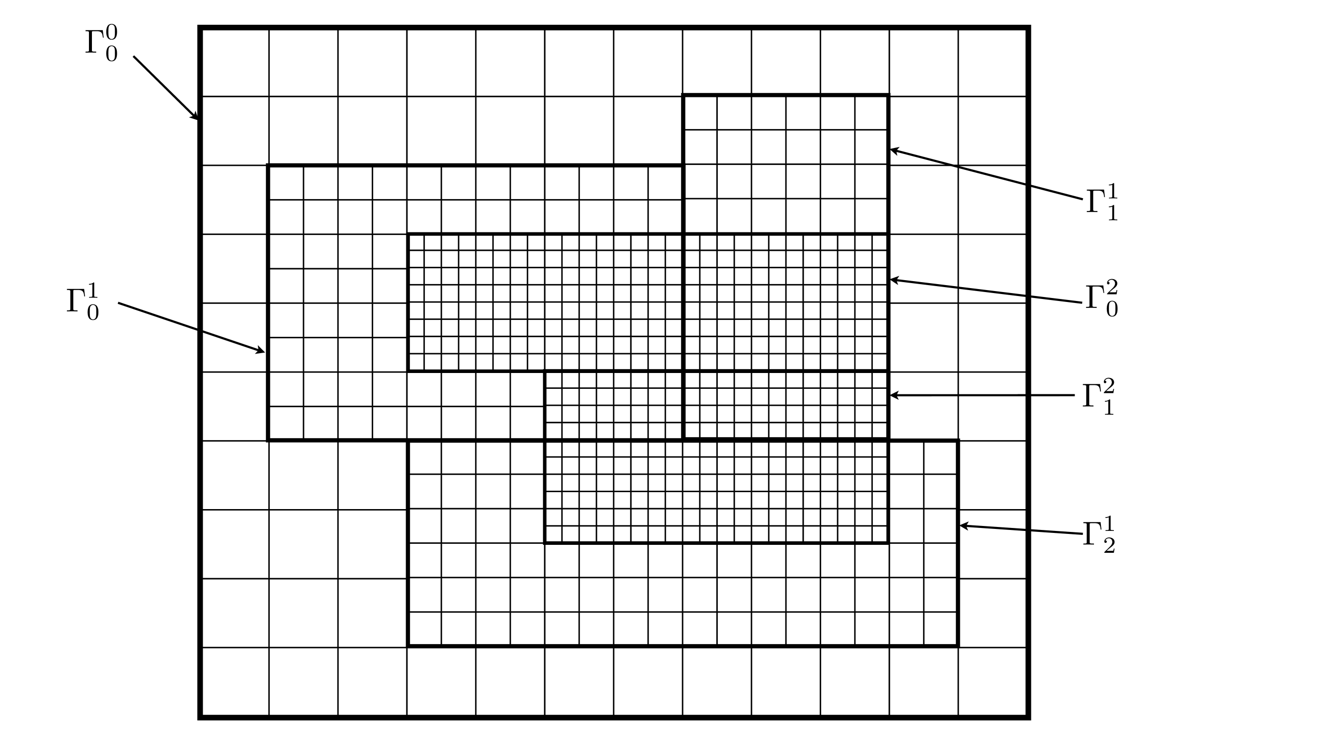
Figure 2: Two-dimensional example of a hierarchy of structured AMR grids. In this case the root level is given by a single subgrid $\Gamma_{0}^{0}$, and is refined by three subgrids $\Gamma^{1}_{0},\Gamma^{1}_{1},\Gamma^{1}_{2}$, generating the first level of refinement. The first level is further refined by two subgrids $\Gamma^{2}_{0}$ and $\Gamma^{2}_{1}$. The refinement level between abutting cells can differ by more than one.

4 The Rendering Algorithm

The outline of our GPU-raycasting algorithm can be summarized as follows:

• First the hierarchy of nested refinement levels is decomposed into non-overlapping, axis-aligned blocks, each covering only cells from the same level of resolution. These are organized in an adaptive kD-tree data structure, encoded using a set of integer-valued 3D textures.

• The data associated with the separate grids are either packed into a single 3D texture or accessed dynamically as individual textures using NVIDIA’s Bindless Texture extension for OpenGL.

• The textures are uploaded onto the GPU and the kD-tree is traversed in the fragment shader. For each pixel the intersections between the viewing ray and the nodes of the kD-tree are computed and the resulting ray-segments are processed in a front-to-back order. The color and opacity contribution of each segment is computed by adaptively sampling the corresponding textures, with a sampling distance based on the underlying level of refinement. The contributions are accumulated to yield the overall pixel color, which is written to the frame-buffer after all segments have been processed.

In the next subsections we will describe these steps in more detail.

4.1 KD-TREE CONSTRUCTION

In order to leverage the capabilities of texturing units on current graphics hardware, e.g. for fast constant or tri-linear interpolation on regular grids, it is beneficial to subdivide the data domain into separate blocks which do not overlap and cover only cells from the same resolution level. Rendering a given hierarchy of separate subgrids directly would result in rendering artifacts, since in the AMR approach the subgrid patches on finer levels do not replace but rather overlay regions of coarser levels, so refined regions of the data volume would be rendered multiple times.

The root node of the kD-tree is defined by the enclosing bounding box ${B}$ of all subgrids $\Gamma^{0}_{i}$ on the root level of the AMR hierarchy. ${B}$ is recursively subdivided by axis-aligned splitting planes, each defining the two child nodes of their parent node. In order to keep the number of generated blocks small, the splitting planes are chosen such that they minimize the number of intersections with the bounding boxes of the subgrids in the domain represented by each node. Therefore we sweep the plane parallel to all three major coordinate planes and determine the number of intersections. The split that introduces the smallest number of intersections and has at least one slab of cells on each side, is chosen. In case several such splits exist, we chose the one that divides the subgrids in the most balanced way, in the sense that the ratio of the number of cells on each side is closest to $1$. The recursion stops, once a node covers only cells from the same subgrid.

Next all subgrids $\Gamma^{1}_{i}$ of the first refinement level are processed. For each leaf node in the current kD-tree we build a list with all the subgrids $\Gamma^{1}_{i}$ that overlap with it. This can be determined efficiently by traversing the current kD-tree top-down starting at the root node, visiting only the child nodes that intersect $\Gamma^{1}_{i}$. Next the kd-tree is refined at each of the resulting leafs, by determining the optimal splitting planes for the blocks defined by the intersections between the subgrids and the region represented by the leaf node as discussed above. This procedure is continued for the other refinement levels, successively extending the tree for each level, until all subgrids $\Gamma^{l}_{i}$ in the hierarchy are processed. A 2D example for the subgrid configuration from Figure 2 is shown in Figure 3. The resulting kD-tree consists of three types of nodes:

1. nodes representing regions of the computational domain with cells that are further refined,

2. nodes that cover only cells that are unrefined, i. e. leaf nodes of the kD-tree, and

3. nodes that cover both, refined and unrefined cells, which are used to traverse the tree in a view-consistent order.

The first type of nodes allows for a level-of-detail selection during the rendering phase, as the corresponding region is covered by at least two levels of resolution. If the resolution of the coarser level is sufficient, which can for example be decided based on the projected screen-space extension of the cells, the node is rendered at this resolution and the traversal is stopped, otherwise the sub-tree of the node is visited.

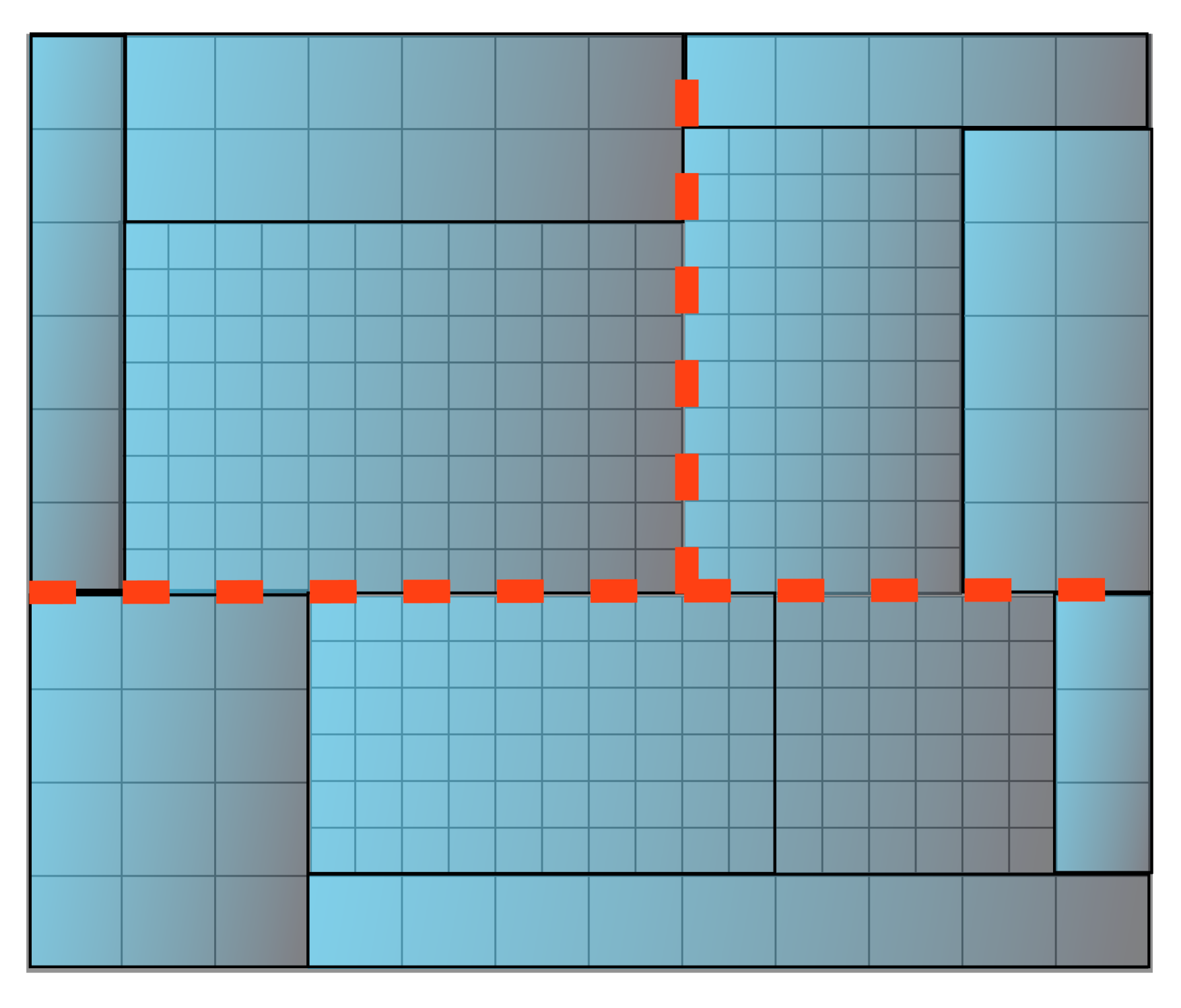
(a)

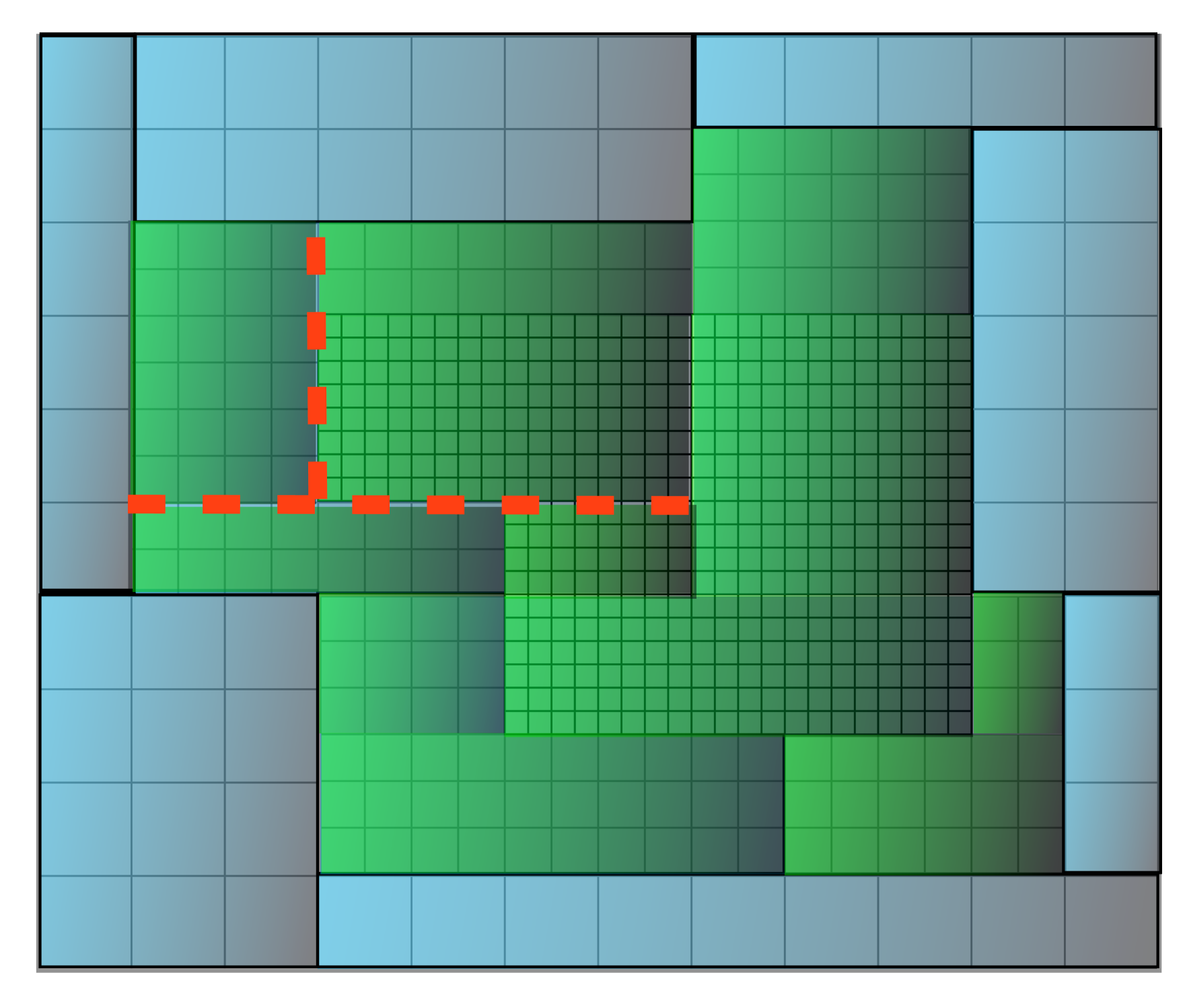
(b)

Figure 3: Two-dimensional example of the decomposition procedure for the AMR hierarchy depicted in Figure 2. Image (a) shows the resulting nodes of the kD-tree after the grids on the first level of refinement have been processed, image (b) shows the tree after all level 2 grids have been taken into account. To avoid cluttering only the first two splitting axis are depicted by the red dotted lines.

No data from the original AMR hierarchy is copied in this process, but rather solely offsets and bounding box information as well as references to the original subgrids are stored with the kD-tree.

4.2 KD-TREE REPRESENTATION ON THE GPU

To traverse the kD-tree structure on the GPU, we represent it by a set of 3D textures. The first texture, called tree texture in the following, encodes the structure of the kD-tree, using one texel for each node. Each texel consists of $64$ bits, split into $32$ bits for the red and green channel. The root node of the tree is stored at texel coordinates $(0,0,0)$. The first two bits of the red-channel encode the orientation of the splitting plane that defines the two child nodes and the next $6$ bits store the level of refinement of the corresponding block of cells. The remaining $24$ bits of the first channel are used to endcode the texel coordinates of the first child node. The second child node is stored at the next sequential texel. As mentioned above the texel coordinate $(0,0,0)$ is reserved for the root note, and we use it to indicate leaf nodes of the tree.

The first $11$ bits of the green-channel store the location of the splitting plane defining the child nodes. By construction of the tree, the splitting planes are always located at the faces of the cells on the particular level of refinement, so we do not need to store its value in floating point coordinates. Instead it is beneficial to use integer coordinates, defined as the number of cells on the current level of refinement, relative to the node’s lower left corner. The remaining $21$ bits of the second channel are used as an index into a second 3D-texture that holds specific information required for nodes of type (a) and (b), see Section 4.1, and will be discussed in the next subsection. A diagram that depicts the specific usage of bits is shown in Figure 4.

A $256^{3}$ index texture, with a memory requirement of $128$ MBytes, is capable of encoding kD-trees with more than $16$ million nodes. The specific choice of bits allows us to distinguish $64$ levels of refinement and subdivision plane positions for nodes covering up to $2048^{3}$ cells on their level of refinement, sufficient for the largest AMR simulations up to date. For moderately sized AMR hierarchies usually a resolution for $128^{3}$ index texture, with memory requirements of only $16$ Mbytes, enabling the storage of more than $2$ million nodes, is sufficient.

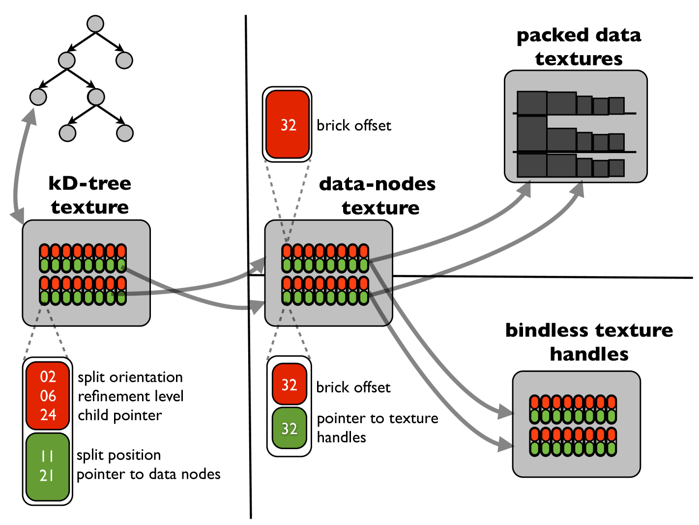
Figure 4: This figure shows the encoding of the kD-tree partition of the data domain using a set of 3D textures. The layout of the tree is stored using an integer valued 3D texture. Nodes of type (a) and (b), see Section 4.1, store indices into a second 3D texture that holds information for accessing the grid data associated with each node. The specific usage of its bits depends on the data storage strategy, see Section 5.

5 DATA STORAGE ON THE GPU

As discussed in Section 4.2, texels for nodes of type (a) or (b), i.e. nodes that represent block of cells that are either completely refined or completely unrefined and thus can be rendered, store an index into a second texture, called data nodes texture in the following. The specific usage of its bits depends on the storage strategy for the data associated with the AMR grids. One challenge for GPU-raycasting of multi-resolution data is that only a limited number of textures can be accessed simultaneously, depending on the number of texture units of the specific graphics hardware. The maximal number is currently about $100$ , far too few to assign a separate texture to each node in the tree structure. Typical AMR simulations generate between $10^{3}$ to $10^{5}$ separate subgrids for each time step. One option to tackle this problem is to use a large 3D texture as a memory pool and copy the data blocks associated with each AMR grid into this texture, which will be discussed in Section 5.0.1. In Subsection 5.0.2 we will discuss an alternative approach, based on NVIDIA’s Bindless Textures extension for OpenGL, [7] available since March 2012, which enables OpenGL applications to dynamically access large number of separate textures in the graphics shaders.

In both cases it is advantageous to assign a separate texture brick per subgrid instead of one brick for each kD-tree nodes of type (a) and (b), because in general there are more kD-tree nodes than subgrids and for higher order interpolation we use a common row of texels at interfaces between adjacent texture blocks. Assigning a separate texture brick per kD-node would drastically increase the number of interfaces and thus texture memory consumption. Furthermore the packing procedure would result in more fragmented areas for a larger number of smaller bricks, see Section 5.0.1 and 6. So we allocate one brick for each AMR subgrid and rather store offsets into these bricks at the nodes of type (a) and (b). We employ nearest-neighbor interpolation for cell-centered AMR data and trilinear interpolation for vertex-centered data. In the first case the texels are aligned with the centers of the cells, while in the second one they are aligned with the vertices of the grid. To avoid artifacts originating from discontinuous tri-linear interpolation between subgrids with different resolutions, adjacent texture-blocks share a row of data samples at their common boundary faces and the data at dangling nodes has to be replaced to the interpolated texel values of the abutting, coarse texture.

5.0.1 TEXTURE PACKING APPROACH

For our purposes the following variant of the three-dimensional packing problem is appropriate: pack a given number of axis-aligned rectilinear boxes into one container with fixed width and depth, such that its height is minimized. [27] This problem belongs to the class of NP-hard problems, but a couple of useful heuristics have been suggested. Similar to the approach discussed in Kaehler et al. [13] we use the so-called next-fit-decreasing-height (NFDH) algorithm. [28] First the texture bricks are inserted into a list, in the order of decreasing extension in the z, y and then x-direction. The packing algorithm starts at the lower left-hand corner of the container and inserts the boxes along the x-axis until the maximal x-extension of the container is reached. A new row is opened, with a y-coordinate given by the largest y-extension of the already inserted boxes. This procedure is repeated until the lowest layer of the container is filled. Then a new layer is in the z-direction is opened and this process continues until all boxes are inserted. We iterate this procedure with different values for the base layer extensions of the container and the result with the smallest volume is chosen. A 3D-texture of this size is defined with the subtextures inserted at their computed positions. Each kD-node of type (a) or (b) in the “data nodes texture”, see upper-right part of Figure 4, stores its offset into the packed texture using 32-bits. This allows to index into a packed texture of up to $2048\times 2048\times 1048$ texels.

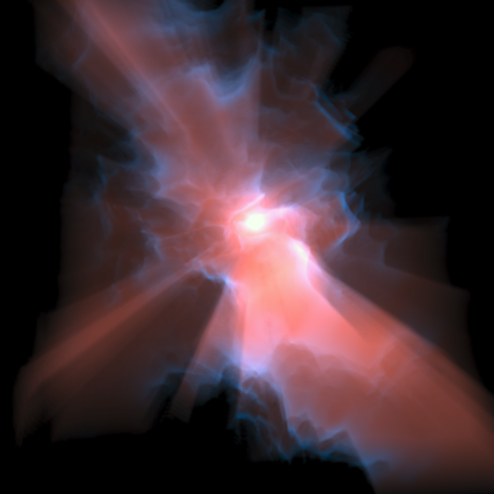
Figure 5: A global illumination example, tracing secondary rays to a central point-light source that illuminates the whole domain.

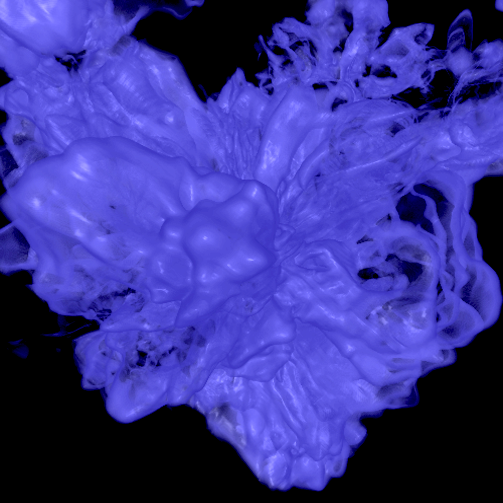
Figure 6: A non-polygonal, semi-transparent iso-surface representation using a gradient-based shading approach, with on-the-fly gradient computation.

5.0.2 DATA ACCESS USING THE BINDLESS TEXTURES EXTENSION

NVIDIA’s Bindless Texture extension [7] allows OpenGL applications to dynamically access large numbers of texture objects in graphics shaders without the need to first bind the textures to specific texture units on the CPU. Instead each texture is identified by a 64-bit handle that is used to sample the texture. This provides a means to manage the large amounts of separate texture bricks associated with typical AMR data structures without the need to pack them into a memory pool. We use 32-bits per texel for the data nodes texture in this case. For each kD-tree node of type (a) and (b) we employ a 32-bit index into another 3D-texture with two 32-bit channels, referred to as the handles textures in the following. It endcodes the $64$-bit texture handles for each texture brick associated with a subgrid, see Figure 4. It is advantageous to store the handles in a separate texture because the number of subgrids is much smaller than the number of kD-nodes, so storing them at each entry in the data nodes texture would introduce an overhead in GPU-memory usage.

5.1 RAY TRAVERSAL

As in the standard GPU-raycasting approach for uniform data [17], we draw the faces of the bounding box enclosing the computational domain to execute an instance of a fragment shader for each covered pixel. In the fragment shader the ray’s origin and direction for the corresponding pixel is computed. Next the segments resulting from the intersection between the viewing ray and the kD-tree data nodes are determined similar to the kD-restart algorithm [29]. The kd-tree texture is sampled starting at the root node with texel coordinate $(0,0,0)$ and traversed top-down, using the child node pointers stored at each node, as discussed in Section 4.2. The bounding box of each node is computed on-the-fly from the extensions of the kD-root node and the orientation and positions of the splitting planes for each node. The split position is mapped from integer-coordinates to the world coordinate system, using the cell size ${\bf h}^{0}$ on the root level, the current level of refinement at the node as well as its bounding box. The traversal continues until either a leaf node is reached, indicated by an “invalid” child node entry of $(0,0,0)$, or until a node of type (a) is visited, which is the case if the node has a valid child node entry and an index into the data nodes texture. The latter case allows for a level-of-detail selection, pruning the traversal of the tree if for example the projected screen size of the cells of this node is below a user-defined threshold.

Next the color and opacity contribution of the corresponding ray-segment is computed. In case of the “packing” approach discussed in Section 5.0.1, the node’s offset into the packed texture is sampled from its entry in the data nodes texture and the ray-segment is transformed to texel coordinates.

In the Bindless Texture approach the current texture handles are read from the handles texture using the index stored in the data nodes texture, and converted to a GLSL sampler3D object. The ray-position is converted to texture coordinates using the number of samples of the texture and the number of texels of the subregion corresponding to the kD-node, which can be computed on-the-fly from its bounding box and the current refinement level. The sampling rate is chosen proportional to the level’s cell-size. When the segment is processed, the kD-tree traversal is “restarted” at the root node and the next ray-segment is visited. Once the total ray is processed, the resulting colors and opacities are written to the frame-buffer.

6 Results and Discussion

The comparison was performed using a NVIDIA GeForce GTX 680 graphics card with $2$ GByte of graphics memory, that was installed on a host with a Intel Xeon E5520 CPU and $24$ GByte main memory. The rendering algorithms were implemented in OpenGL and the OpenGL Shading Language (GLSL). We tested the performance and memory requirements of the proposed algorithms on three datasets with different sizes and characteristics. All performance measurements refer to a viewport size of $1000^{2}$ pixels. Table 1 lists information about the datasets and the corresponding kD-trees: the number of subgrids, refinement levels and cells in the original SAMR grid hierarchies as well as the total number of nodes in the resulting kD-trees and the portion of nodes of type (b) and (c), see Section 4.1.

Table 1: The characteristics of the datasets: the number of subgrids, refinement levels, cells as well as the total number of nodes in the resulting kD-trees and the portion of internal and leaf nodes that are associated with blocks of cells.

	#grids	#levels	#cells	#kd-tree nodes	#kd-data nodes
dataset 1	2,666	4	$19\times 10^{6}$	30,096	27,249
dataset 2	18,528	4	$33\times 10^{6}$	178,114	162,095
dataset 3	39,061	13	$140\times 10^{6}$	368,225	343,389

We compared the two single-pass rendering methods proposed in this paper to a multi-pass approach [18], that traverses the kD-tree on the CPU and renders each data node separately, by first binding the associated texture to a texture unit and rendering the bounding box of the kD-tree node to initialize the fragment shaders. The kD-tree partition approach described in Section 4.1 was used for all three methods. Table 2 shows the GPU memory requirements, preprocessing times and performance numbers for the different rendering methods. The numbers in each cell of the table are the measurements for the three different datasets. For the packing and the bindless textures approach the first number in the “GPU memory” column is the size of the set of the 3D integer textures used to encode the kD-tree structure and the data nodes, whereas the second number gives the memory requirements for the grid data, i. e. the packed texture or the sum of the separate 3D-textures in the bindless case. An emission-absorption model with no further acceleration techniques, like early-ray-termination or empty-space-skipping, was used in the examples. Renderings of the different datasets are shown in Figure 7.

Table 2: GPU memory requirements, preprocessing times and performance numbers for the three different rendering methods. The numbers in each table cell are measurements for the three different datasets shown in Table 1 and Figure 7.

	GPU memory [Mbytes]			preprocessing[s]			performance [fps]
multi-pass	71.4	124.2	530.3	1.1	2.6	6.8	4.2	2.1	0.8
packing	0.5 + 239.3	2.7 + 310.3	4.3 + 1000.2	3.4	7.5	8.1	3.2	1.6	1.2
bindless-texture	0.5 + 71.4	2.8 + 124.2	6.1 + 530.3	1.7	3.2	7.4	2.1	0.9	0.4

As indicated by the measurements shown in Table 2 the rendering performance of the packing approach is faster than the bindless texture approach for all examples, due to the overhead associated with the dynamic access of the separate textures in the bindless texture case. However, the packing approach uses more texture memory, as the packing of the differently sized subgrid textures into the texture memory pool necessarily introduces some fragmentation. An efficiency, defined as the number of used texels to the total number of texels in the packed texture, between 30% and 50% was achieved for the three datasets. The multi-pass approach has faster rendering performance for the smallest and the medium sized dataset 1 and 2, but the packing approach is about 50% faster for the largest dataset, number 3. Here the cost of the per-pixel sampling of the kD-tree structure is lower than the overhead for binding of the separate textures and rendering the bounding boxes of each kD-node to initialize the fragment shader instances in the multi-pass approach.

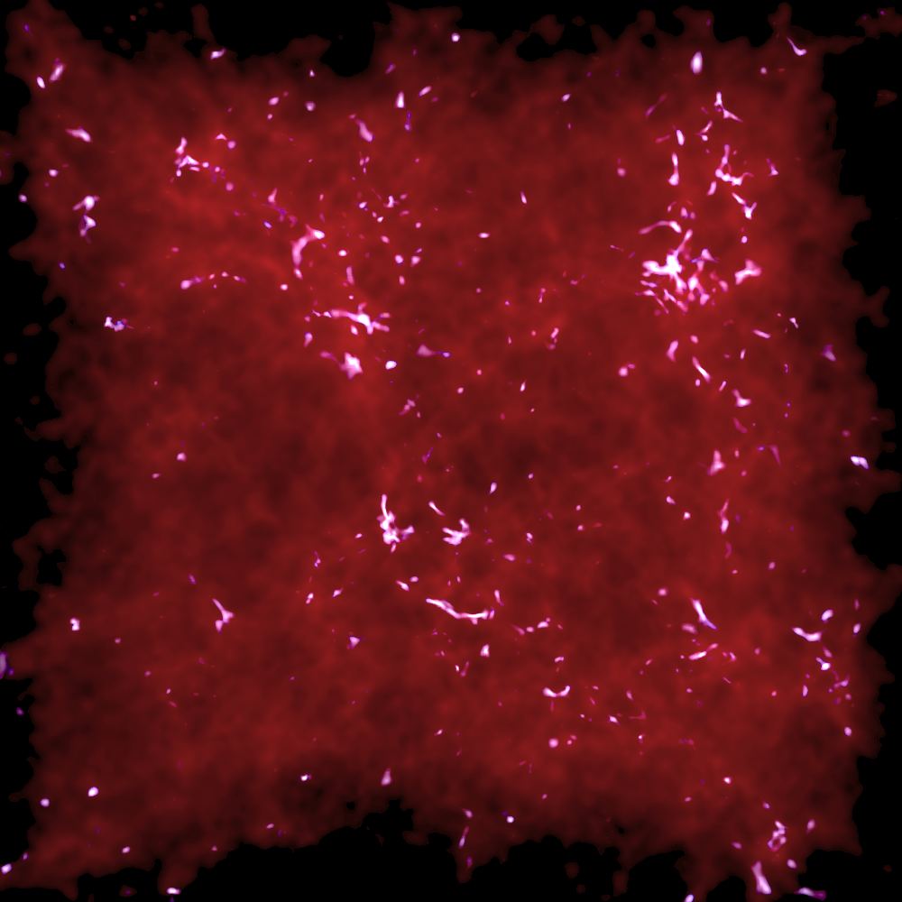
(a)

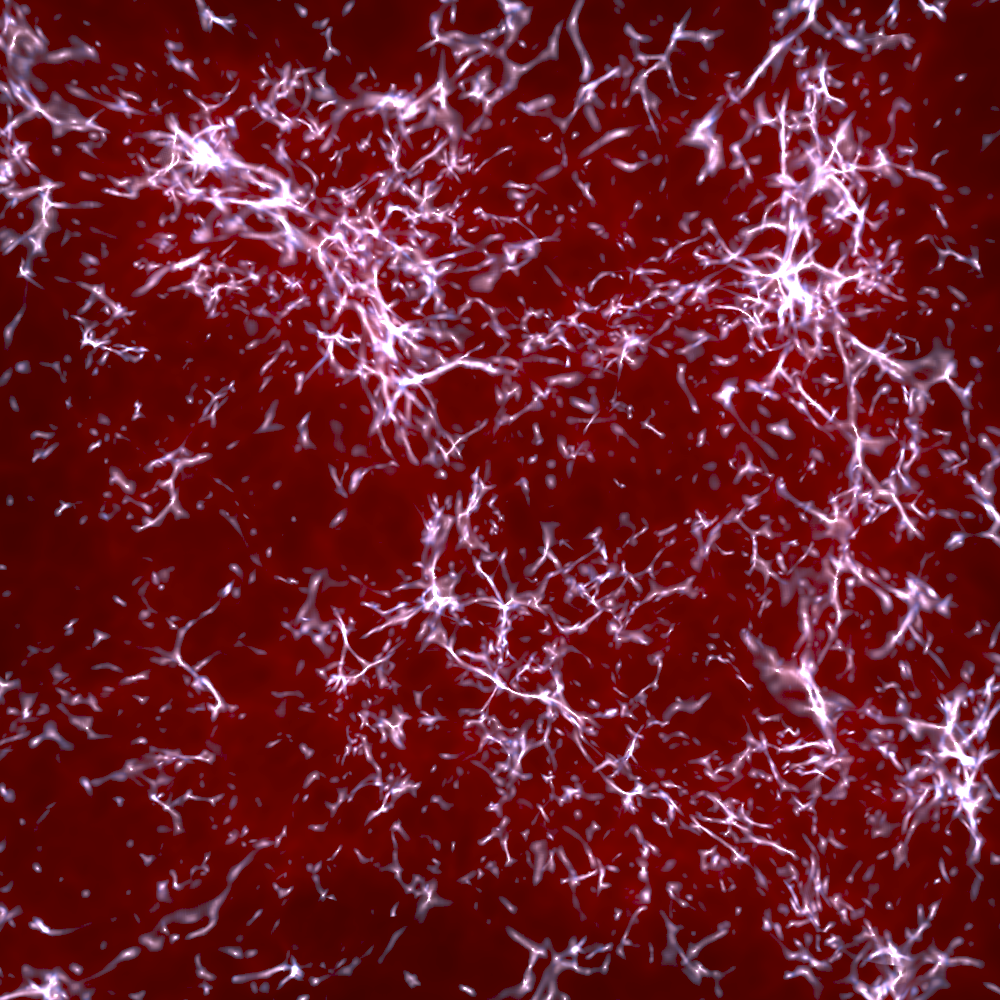
(b)

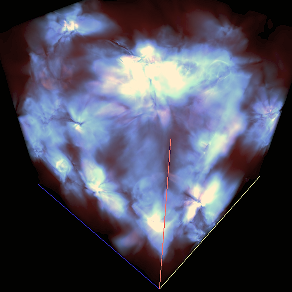
(c)

Figure 7: Renderings of the three different data sets used in this paper. Image (a) and (b) show the large scale distribution of hydrogen gas on scales of 100 Mpc at two different time steps. Image (c) shows the temperature distribution between dwarf galaxies that formed in the early Universe. Information about the datasets can be found in Table 1.

Unlike the multipass approach the single-pass methods allow the application of advanced lighting schemes, that require simultaneous access to more than one kD-tree node. Two examples for dataset 3 are shown in Figure 5 and 6. Figure 6 is a non-polygonal semi-transparent iso-surface representation using a gradient-based shading approach, rendered at $0.8$ fps. The gradients were computed on-the-fly. Figure 5 shows a global illumination example. Here for each sampling location a secondary ray is traced to a central point-like light source. The achieved frame rate was $0.1$ fps.

7 Conclusions

We presented a single-pass GPU-raycasting approach for Structured Adaptive Mesh Refinement (SAMR) data. It employs a kD-tree to subdivide the data domain into axis-aligned, non-overlapping blocks of cells from the same resolution level. The tree is encoded by a set of 3D-textures, which allows to efficiently traverse it entirely on the GPU. We discussed two different data access strategies, namely a “packing” approach using a texture memory pool, and a method based on NVIDIA’s Bindless Texture extension for OpenGL, and applied them to several SAMR datasets of different sizes and complexity.

For all examples the 3D textures used to encode the kD-tree structure required only small amounts of texture memory. The packing approach offers higher rendering performance as long as all data fits into texture memory, because of the extra costs of the dynamically accessing the separate textures in the Bindless Texture approach, whereas the latter consumes less texture memory. We further compared the new approaches to a previously published multi-pass method [18]. For complex and large SAMR datasets the packing approach outperformed the multi-pass algorithm and in contrast to the latter, both new methods enable a straight-forward implementation of many advanced shading and acceleration techniques, since all parts of the data domain are accessible in the fragment shader. They further do not suffer from read-after-write hazards as multi-pass approaches that use non-standard blending equations and need to read back from the frame-buffer for each pass, or apply synchronization methods, which substantially decrease the rendering performance. Because the new single-pass methods are executed entirely on the GPU without any CPU interaction, their rendering performance should directly benefit from the increased number of shader cores expected for upcoming GPU generations. The bindless texture approach is especially well suited for datasets that exceed the available graphics memory, as it allows to dynamically upload subsets of textures as required by out-of-core rendering approaches.

8 Acknowledgments

We would like to thank Ziba Mahdavi (KIPAC) and Shalini Venkataraman (NVIDIA) for providing us with $NVIDIA$ $Kepler$ GPUs. We also thank Ji-hoon Kim (UCSC) and John Wise (Georgia Tech) for the datasets used to test the presented algorithms. This work was supported in part by the National Science Foundation through award number AST-0808398 and the LDRD program at the SLAC National Accelerator Laboratory as well as the Terman fellowship at Stanford University.

References

- [1] Turk, M. J., Abel, T., and O’Shea, B., “The formation of Population III binaries from cosmological initial conditions.,” Science 325(5940), 601–5 (2009).
- [2] Abel, T., Bryan, G. L., and Norman, M. L., “The Formation of the First Star in the Universe,” Science 295, 93–98 (Jan. 2002).
- [3] Berger, M. J. and Oliger, J., “Adaptive mesh refinement for hyperbolic partial equations,” Journal of Computational Physics 53, 484–512 (1984).
- [4] Kaehler, R. and Hege, H.-C., “Texure-based Volume Rendering of Adaptive Mesh Refinement Data,” The Visual Computer 18(8), 481–492 (2002).
- [5] Jankun-Kelly, T. J., Kreylos, O., Shalf, J. M., Ma, K.-L., Hamann, B., Joy, K. I., and Bethel, E. W., “Deploying web-based visual exploration tools on the grid,” IEEE Computer Graphics and Applications 23(2), 40–50 (2003).
- [6] Weber, G. H., Kreylos, O., Ligocki, T. J., Shalf, J. M., Hagen, H., Hamann, B., and Joy, K. I., “High-quality volume rendering of adaptive mesh refinement data,” in [Proceedings of Vision, Modeling, and Visualization 2001 ], 121–128 (Stuttgart, Germany, 2001).
- [7] NVIDIA, “Bindless Texture OpenGL Extension.” http://www.opengl.org/registry/specs/NV/bindless_texture.txt (2012).
- [8] Max, N. L., “Sorting for polyhedron composition,” In H. Hagen, H. Müller, G. M. Nielson: Focus on Scientific Visualization, Springer Verlag , 259–268 (1993).
- [9] Weber, G. H., Kreylos, O., Ligocki, T. J., Shalf, J. M., Hagen, H., Hamann, B., and Joy, K. I., “Extraction of crack-free isosurfaces from adaptive mesh refinement data,” in [Data Visualization 2001 (Proceedings of VisSym ’01) ], 25–34 (2001).
- [10] Moran, P. and Ellsworth, D., “Visualization of amr data with multi-level dual-mesh interpolation,” IEEE Transactions on Visualization and Computer Graphics 17, 1862–1871 (2011).
- [11] Weber, G. H., Oehler, M., Kreylos, O., Shalf, J. M., Bethel, W., Hamann, B., and Scheuermann, G., “Parallel cell projection rendering of adaptive mesh refinement data,” in [Proceeding of the IEEE Symposium on Parallel and Large-Data Visualization and Graphics ], Koning, A., Machiraju, R., and Silva, C. T., eds., 51–60, IEEE, IEEE Computer Society Press, Los Alamitos, California (2003).
- [12] Turk, M. J., Smith, B. D., Oishi, J. S., Skory, S., Skillman, S. W., Abel, T., and Norman, M. L., “yt: A multi-code analysis toolkit for astrophysical simulation data,” The Astrophysical Journal Supplement Series 192(1), 9 (2011).
- [13] Kaehler, R., Simon, M., and Hege, H.-C., “Fast Volume Rendering of Sparse Datasets using Adaptive Mesh Refinement,” IEEE Transactions on Visualization and Computer Graphics 9(3), 341–351 (2003).
- [14] Park, S., Bajaj, C. L., and Siddavanahalli, V., “Case study: Interactive rendering of adaptive mesh refinement data,” in [Proceedings of IEEE Visualization ], Moorhead, R., Gross, M., and Joy, K. I., eds., 521–524, IEEE Computer Society Press (2002).
- [15] Roettger, S., Guthe, S., Weiskopf, D., Ertl, T., and Strasser, W., “Smart hardware-accelerated volume rendering,” in [VISSYM ’03: Proceedings of the symposium on Data visualisation 2003 ], 231–238, Eurographics Association, Aire-la-Ville, Switzerland, Switzerland (2003).
- [16] Krueger, J. and Westermann, R., “Acceleration techniques for GPU-based volume rendering,” in [VIS ’03: Proceedings of the 14th IEEE Visualization 2003 (VIS’03) ], 38, IEEE Computer Society, Washington, DC, USA (2003).
- [17] Stegmaier, S., Strengert, M., Klein, T., and Ertl, T., “A simple and flexible Volume Rendering Framework for Graphics-Hardware-based Raycasting,” in [Fourth International Workshop on Volume Graphics ], 187– 241 (2005).
- [18] Kaehler, R., Wise, J., Abel, T., and Hege, H.-C., “GPU-Assisted Raycasting for Cosmological Adaptive Mesh Refinement Simulations,” in [International Workshop on Volume Graphics 2006 ], 103–110, Eurographics / IEEE VGTC 2006, Boston (2006).
- [19] Ljung, P., “Adaptive Sampling in Single Pass, GPU-based Raycasting of Multiresolution Volumes,” in [Proceedings of the International Workshop on Volume Graphics 2006 ], 39–46, Eurographics / IEEE VGTC 2006, Boston (30 - 31 July 2006).
- [20] Vollrath, J. E., Schafhitzel, T., and Ertl, T., “Employing Complex GPU Data Structures for the Interactive Visualization of Adaptive Mesh Refinement Data,” in [Proceedings of the International Workshop on Volume Graphics 2006 ], 55–58, Eurographics / IEEE VGTC 2006, Boston (30 - 31 July 2006).
- [21] Gobbetti, E., Marton, F., and Iglesias Guitin, J. A., “A single-pass gpu ray casting framework for interactive out-of-core rendering of massive volumetric datasets,” Vis. Comput. 24, 797–806 (July 2008).
- [22] Crassin, C., Neyret, F., Lefebvre, S., and Eisemann, E., “Gigavoxels : Ray-guided streaming for efficient and detailed voxel rendering,” in [ACM SIGGRAPH Symposium on Interactive 3D Graphics and Games (I3D) ], ACM, ACM Press, Boston, MA, Etats-Unis (feb 2009). to appear.
- [23] Marchesin, S. and de Verdiere, G. C., “High-quality, semi-analytical volume rendering for amr data,” IEEE Transactions on Visualization and Computer Graphics 15, 1611–1618 (Nov. 2009).
- [24] Berger, M. J. and Collela, P., “Local adaptive mesh refinement for shock hydrodynamics,” J. Computational Physics 82(1), 64–84 (1989).
- [25] Abel, T., Bryan, G., and Norman, M. L., “The formation of the first star in the universe,” Science 295, issue 5552, 93–98 (2002).
- [26] O’Shea, B. W., Bryan, G., Bordner, J., Norman, M. L., Abel, T., Harkness, R., and Kritsuk, A., “Introducing Enzo, an AMR Cosmology Application,” ArXiv Astrophysics e-prints (Mar. 2004).
- [27] Li, K. and Cheng, K.-H., “On three-dimensional packing,” SIAM Journal on Computing 19(5), 847–867 (1990).
- [28] Johnson, D. S., E. G. Coffman, Jr., Garey, M. R., and Tarjan, R. E., “Performance bounds for level-oriented two dimensional packing algorithms,” SIAM Journal on Computing 9, 808–826 (1980).
- [29] Horn, D. R., Sugerman, J., Houston, M., and Hanrahan, P., “Interactive k-d tree gpu raytracing,” in [Proceedings of the 2007 symposium on Interactive 3D graphics and games ], I3D ’07, 167–174, ACM, New York, NY, USA (2007).