Lectures on integrable probability

Abstract

These are lecture notes for a mini-course given at the St. Petersburg School in Probability and Statistical Physics in June 2012. Topics include integrable models of random growth, determinantal point processes, Schur processes and Markov dynamics on them, Macdonald processes and their application to asymptotics of directed polymers in random media.

Preface

These lectures are about probabilistic systems that can be analyzed by essentially algebraic methods.

The historically first example of such a system goes back to De Moivre (1738) and Laplace (1812) who considered the problem of finding the asymptotic distribution of a sum of i.i.d. random variables for Bernoulli trials, when the pre-limit distribution is explicit, and took the limit of the resulting expression. While this computation may look like a simple exercise when viewed from the heights of modern probability, in its time it likely served the role of a key stepping stone — first rigorous proofs of central limit theorems appeared only in the beginning of the XXth century.

At the moment we are arguably in a ‘‘De Moivre-Laplace stage’’ for a certain class of stochastic systems which is often referred to as the KPZ universality class, after an influential work of Kardar-Parisi-Zhang in mid-80’s. We will be mostly interested in the case of one space dimension. The class includes models of random growth that have built-in mechanisms of smoothing and lateral growth, as well as directed polymers in space-time uncorrelated random media and driven diffusive lattice gases.

While the class and some of its members have been identified by physicists, the first examples of convincing (actually, rigorous) analysis were provided by mathematicians, who were also able to identify the distributions that play the role of the Gaussian law. Nowadays, they are often referred to as the Tracy-Widom type distributions as they had previously appeared in Tracy-Widom’s work on spectra of large random matrices.

The reason for mathematicians’ success was that there is an unusually extensive amount of algebra and combinatorics required to gain access to suitable pre-limit formulas that admit large time limit transitions. As we will argue below, the ‘‘solvable’’ or integrable members of the class should be viewed as projections of much more powerful objects whose origins lie in representation theory. In a way, this is similar to integrable systems that can also be viewed as projections of representation theoretic objects; and this is one reason we use the words integrable probability to describe the phenomenon. There are also much more direct links between integrable systems and integrable probability some of which we mention below.

The goal of these notes is not to give a survey of a variety of integrable probabilistic models that are known by now (there are quite a few, and not all of them are members of the KPZ universality class), but rather to give a taste of them by outlining some of the algebraic mechanisms that lead to their solution.

The notes are organized as follows.

In Section 1 we give a brief and non-exhaustive overview of the integrable members of the KPZ universality class in (1+1) dimensions.

In Section 2 we provide the basics of the theory of symmetric functions that may be seen as a language of the classical representation theory.

In Section 3 we discuss determinantal random point processes — a fairly recent class of point processes that proved very effective for the analysis of growth models and also for the analysis of integrable probabilistic models of random matrix type.

Section 4 explains a link between a particular random growth model (known as the polynuclear growth process or PNG) and the so-called Plancherel measures on partitions that originates from representation theory of symmetric groups.

In Section 5 we introduce a general class of the Schur measures that includes the Plancherel measures; members of these class can be viewed as determinantal point processes, which provides a key to their analysis. We also perform such an analysis in the case of the Plancherel measure, thus providing a proof of the celebrated Baik-Deift-Johansson theorem on asymptotics of longest increasing subsequences of random permutations.

Section 6 explains how integrable models of stochastic growth can be constructed with representation theoretic tools, using the theory of symmetric functions developed earlier.

In Section 7 we show how one can use celebrated Macdonald symmetric functions to access the problem of asymptotic behavior of certain directed random polymers in (1+1) dimensions (known as the O’Connell-Yor polymers). The key feature here is that the formalism of determinantal processes does not apply, and one needs to use other tools that here boil down to employing Macdonald-Ruijsenaars difference operators.

1 Introduction

Suppose that you are building a tower out of unit blocks. Blocks are falling from the sky, as shown at Figure 1 (left picture) and the tower slowly grows. If you introduce randomness here by declaring the times between arrivals of blocks to be independent identically distributed (i.i.d.) random variables, then you get the simplest 1d random growth model. The kind of question we would like to answer here is what the height $h(t)$ of tower at time $t$ is?

The classical central limit theorem (see e.g. [Billingsley-95, Chapter 5] or [Kallenberg-02, Chapter 4]) provides the answer:

$$h(t)\approx c_{1}^{-1}t+\xi c_{2}c_{1}^{-\frac{3}{2}}t^{\frac{1}{2}},$$

where $c_{1}$ and $c_{2}$ are the mean and standard deviation of the times between arrivals of the blocks, respectively, and $\xi$ is a standard normal random variable $N(0,1)$.

Figure 1: Growth models based on the falling boxes: 1d model, 2d model without interactions, 2d model with sticky boxes (ballistic deposition)

If blocks fall independently in different columns, then we get a 2d growth model, as shown at Figure 1 (middle picture). When there are no interactions between blocks and the blocks are aligned, the columns grow independently and fluctuations remain of order $t^{1/2}$. But what happens if we make blocks sticky so that they get glued to the boxes of adjacent columns, as shown at Figure 1 (right picture)? This model is known as ballistic deposition and, in general, the answer for it is unknown. However, computer simulations (see e.g. [Barabasi-Stanley-95]) show that the height fluctuations in this model are of order $t^{1/3}$, and the same happens when the interaction is introduced in various other ways. Perhaps, there is also some form of a Central Limit Theorem for this model, but nobody knows how to prove it.

Coming back to the 1d case, one attempt to guess the central limit theorem would be through choosing certain very special random variables. If the times between arrivals are geometrically distributed random variables, then $h(t)$ becomes the sum of independent Bernoulli random variables and the application of the Stirling’s formula proves the convergence of rescaled $h(t)$ to the standard Gaussian. (This is the famous De Moivre–Laplace theorem.)

In the 2d case it is also possible to introduce particular models for which we can prove something. Consider the interface which is a broken line with slopes $\pm 1$, as shown at Figure 2 (left picture) and suppose that a new unit box is added at each local minimum independently after an exponential waiting time.

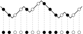
Figure 2: Broken line with slopes $\pm 1$, local minimum where a box can be added, and correspondence with particle configurations on $\mathbb{Z}$.

There is also an equivalent formulation of this growth model. Project the interface to a straight line and put ‘‘particles’’ at projections of unit segments of slope $-1$ and ‘‘holes’’ at projections of segments of slope $+1$, see Figure 2 (right picture). Now each particle independently jumps to the right after an exponential waiting time (put it otherwise, each particle jumps with probability $dt$ in each very small time interval $[t,t+dt]$) except for the exclusion constraint: Jumps to the already occupied spots are prohibited. This is a simplified model of a one-lane highway which is known under the name of Totally Asymmetric Simple Exclusion Process (TASEP), cf. [Spitzer-70], [Liggett-85], [Liggett-99].

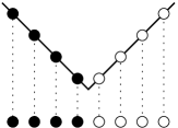
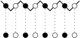
Figure 3: Wedge and flat initial conditions: broken lines and corresponding particle configurations.

Theorem 1.1 ([Johansson-00]).

Suppose that at time $0$ the interface $h(x;t)$ is a wedge ($h(x,0)=|x|$) as shown at Figure 3 (left picture). Then for every $x\in(-1,1)$

$$\lim_{t\to\infty}\mathbb{P}\left(\frac{h(t,tx)-c_{1}(x)t}{c_{2}(x)t^{1/3}}\geq-s\right)=F_{2}(s),$$

where $c_{1}(x)$, $c_{2}(x)$ are certain (explicit) functions of $x$.

Theorem 1.2 ([Sasamoto-05], [Borodin-Ferrari-Prähofer-Sasamoto-07]).

Suppose that at time $0$ the interface $h(x;t)$ is flat as shown at Figure 3 (right picture). Then for every $x\in\mathbb{R}$

$$\lim_{t\to\infty}\mathbb{P}\left(\frac{h(t,x)-c_{3}t}{c_{4}t^{1/3}}\geq-s\right)=F_{1}(s),$$

where $c_{3}$, $c_{4}$ are certain (explicit) positive constants.

Here $F_{1}(s)$ and $F_{2}(s)$ are distributions from random matrix theory, known under the name of Tracy-Widom distributions. They are the limiting distributions for the largest eigenvalues in Gaussian Orthogonal Ensemble and Gaussian Unitary Ensemble of random matrices (which are the probability measures with density proportional to $\exp(-Trace(X^{2}))$ on real symmetric and Hermitian matrices, respectively), see [Tracy-Widom-94], [Tracy-Widom-96].

These two theorems give the conjectural answer for the whole ‘‘universality class’’ of 2d random growth models, which is usually referred to as the KPZ (Kardar-Parisi-Zhang) universality class. Comparing to the answer in the 1d case we see that the asymptotic behavior becomes more delicate — while scaling by $t^{1/3}$ is always the same, the resulting distribution may also depend on the ‘‘subclass’’ of our model. Also, conjecturally, the only two generic subclasses are the ones we have seen. They are distinguished by whether the global surface profile is locally curved or flat near the observation location.

Let us concentrate on the wedge initial condition. In this case there is yet another reformulation of the model. Write in each box $(i,j)$ of the positive quadrant a random ‘‘waiting time’’ $w_{(i,j)}$. Once our random interface (of type pictured in Figure 2) reaches the box $(i,j)$ it takes time $w_{(i,j)}$ for it to absorb the box. Now the whole quadrant is filled with nonnegative i.i.d. random variables. How to reconstruct the growth of the interface from these numbers? More precisely, at what time $T(i,j)$ a given box $(i,j)$ is absorbed by the growing interface? A simple argument shows that

$$T(i,j)=\max\limits_{(1,1)=b[1]\to b[2]\to\dots b[i+j-1]=(i,j)}\sum_{k=1}^{i+j-1}w_{b[k]},$$ (1.1)

where the sum is taken over all directed (leading away from the origin) paths joining $(1,1)$ and $(i,j)$, see Figure 4. The quantity (1.1) is known as the (directed) Last Passage Percolation time. Indeed, if you think about numbers $w_{(i,j)}$ as of times needed to percolate into a given box, then (1.1) gives the time to percolate from $(1,1)$ in $(i,j)$ in the worst case scenario.

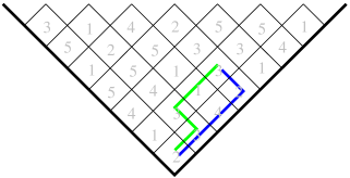
Figure 4: The quadrant filled with waiting times and two (out of ${4\choose 1}=4$ possibilities) directed paths joining $(1,1)$ and $(4,1)$.

Universality considerations make one believe that the limit behavior of the Last Passage Percolation time should not depend on the distribution of $w_{(i,j)}$ (if this distribution is not too wild), but we are very far from proving this at the moment. However, again, the Last Passage Percolation time asymptotics has been computed for certain distributions, e.g. for the exponential distribution in the context of Theorem 1.1.

Let us present another example, where the (conjecturally, universal) result can be rigorously proven. Consider the homogeneous, density 1 Poisson point process in the first quadrant, and let $L(\theta)$ be the maximal number of points one can collect along a North-East path from $(0,0)$ to $(\theta,\theta)$, as shown at Figure 5.

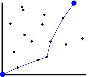
Figure 5: The Poisson point process in the first quadrant and a North–East path joining $(0,0)$ and $(\theta,\theta)$ and collecting maximal number of points, which is $5$ here.

This quantity can be seen as a limit of the LPP times when $w_{(i,j)}$ takes only two values $0$ and $1$, and the probability of $1$ is very small. Such considerations explain that $L(\theta)$ should be also in the KPZ universality class. And, indeed, this is true.

Theorem 1.3 ([Baik-Deift-Johansson-99]).

$$\lim_{\theta\to\infty}\mathbb{P}\left(\frac{L(\theta)-2\theta}{\theta^{1/3}}\leq s\right)=F_{2}(s).$$

It is not hard to show that Theorem 1.3 is equivalent to

Theorem 1.4 ([Baik-Deift-Johansson-99]).

Let $\sigma$ be a uniformly distributed permutation of the set $\{1,\dots,n\}$, and let $\ell_{n}(\sigma)$ be the length of the longest increasing subsequence of $\sigma$. Then

$$\lim_{n\to\infty}\mathbb{P}\left(\frac{\ell_{n}-2\sqrt{n}}{n^{1/6}}\leq s\right)=F_{2}(s).$$

The problem of understanding the limit behavior of $\ell_{n}$ has a long history and goes back to the book of Ulam of 1961 [Ulam-61]. Ulam conjectured that $\mathbb{E}\ell_{n}\approx c\sqrt{n}$ but was not able to identify the constant; he also conjectured Gaussian fluctuations. In 1974 Hammersley [Hammersley-72] proved, via a sub–additivity argument, that there exists a constant such that $\ell_{n}\approx c\sqrt{n}$ and this constant was identified in 1977 by Kerov and Vershik [Vershik-Kerov-77].

The random variable $\ell_{n}$ has an interesting interpretation in terms of an airplane boarding problem. Imagine a simplified airplane with one seat in each of $n$ rows, large distances between rows, and one entrance in front. Each entering passenger has a ticket with a seat number, but the order of passengers in the initial queue is random (this is our random permutation). Suppose that each passenger has a carry-on, and it takes one minute for that person to load it into the overhead bin as soon as (s)he reaches her/his seat. The aisle is narrow, and nobody can pass the passenger who is loading the carry-on. It turns out that the total time to board the airplane is precisely $\ell_{n}$. Let us demonstrate this with an example.

Consider the permutation $\sigma=2413$ with $\ell_{4}(\sigma)=2$. The airplane boarding looks as follows: The first passenger enters the airplane and proceeds to the seat number $2$. While (s)he loads a carry-on, the other passengers stay behind and the one with the ticket for the seat number $1$ ((s)he was the third person in the original queue) starts loading her/his carry-on. After one minute, the passenger with the ticket for the seat number $4$ proceeds to his seat and also starts loading, as well as the one aiming for the seat number $3$. In two minutes the boarding is complete.

Interestingly enough, if the queue is divided into groups, as often happens in reality, then the boarding time (for long queues) will only increase by the factor $\sqrt{k}$, where $k$ is the number of the groups.

Let us now proceed to more recent developments. In the Last Passage Percolation problem we were maximizing a functional $H(x)$ over a set $\mathcal{X}$. A general statistical mechanics principle says that such a maximization can be seen as zero-temperature limit of the Gibbs ensemble on $\mathcal{X}$ with Hamiltonian $-H(x)$. More formally, we have the following essentially obvious statement

$$\max_{x\in\mathcal{X}}H(x)=\lim_{\beta\to\infty}\frac{1}{\beta}\ln\sum_{x\in\mathcal{X}}e^{\beta H(x)}.$$

The parameter $\beta$ is usually referred to as the inverse temperature in the statistical mechanics literature.

In the Last Passage Percolation model, $\mathcal{X}$ is the set of all directed paths joining $(1,1)$ with a point $(a,b)$, and the value of $H$ on path $x$ is the sum of $w_{(i,j)}$ along the path $x$. The Gibbs ensemble in this case is known under the name of a ‘‘Directed Polymer in Random Media’’. The study of such objects with various path sets and various choices of noise (i.e. $w_{(i,j)}$) is a very rich subject.

Directed Polymers in Random Media appeared for the first time close to thirty years ago in an investigation of low temperature expansion of the partition function of the Ising model with domain wall boundary conditions, see [Huse-Henley-85], [Imbrie-Spenser-88], but nowadays there are many other physical applications. Let us give one concrete model where such polymers arise.

Consider a set of massive particles in $\mathbb{Z}$ that evolve in discrete time as follows. At each time moment the mass of each particle is multiplied by a random variable $d_{t,x}$, where $t$ is the time moment and $x$ is the particle’s position. Random variables $d_{t,x}$ are typically assumed to be i.i.d. Then each particle gives birth to a twin of the same mass and the twin moves to $x+1$. If we now start at time $0$ with a single particle of mass $1$ at $x=1$, then the mass $Z(T,x)$ of all particles at $x$ at time $T$ can be computed as a sum over all directed paths $(1,1)=b[1]\to b[2]\to\dots b[x+T-1]=(T,x)$ joining $(1,1)$ and $(T,x)$:

$$Z(T,x)=\sum\limits_{(1,1)=b[1]\to b[2]\to\dots b[x+T-1]=(T,x)}\prod_{k=1}^{x+T-1}d_{b[k]},$$ (1.2)

This model can be used as a simplified description for the migration of plankton with $d_{t,x}$ representing the state of the ocean at location $x$ and time $t$ which affects the speed of growth of the population. Independent $d_{t,x}$ model quickly changing media, e.g. due to the turbulent flows in the ocean.

Random Polymers in Random Media exhibit a very interesting phenomenon called intermittency which is the existence of large peeks happening with small probability, that are high enough to dominate the asymptotics of the moments. Physicists believe that intermittency is widespread in nature and, for instance, the mass distribution in the universe or a magnetogram of the sun show intermittent behavior. To see this phenomenon in our model, suppose for a moment that $d_{t,x}$ does not depend on $t$. Then there would be locations where the amount of plankton exponentially grows, while in other places all the plankton quickly dies, so we see very high peaks. Now it is reasonable to expect that such peaks would still be present when $d_{t,x}$ are independent both of $t$ and $x$ and this will cause intermittency. Proving and quantifying intermittency is, however, rather difficult.

Regarding the distribution of $Z(T,x)$, it was long believed in the physics literature that it should belong to the same KPZ universality class as the Last Passage Percolation. Now, at least in certain cases, we can prove it. The following integrable random polymer was introduced and studied by Seppäläinen [Seppäläinen-12] who proved the $t^{\frac{1}{3}}$ exponent for the fluctuations. The next theorem is a refinement of this result.

Theorem 1.5 ([Borodin-Corwin-Remenik-12]).

Assume $d_{t,x}$ are independent positive random variables with density

$$\frac{1}{\Gamma(\theta)}x^{-\theta-1}\exp\left(-\frac{1}{x}\right).$$

Then there exist $\theta^{*}>0$ and (explicit) $c_{1},c_{2}>0$ such that for $0<\theta<\theta^{*}$,

$$\lim_{n\to\infty}\mathbb{P}\left(\frac{Z(n,n)-c_{1}n}{c_{2}n^{1/3}}\leq s\right)=F_{2}(s).$$

The upper bound on the parameter $\theta>0$ in this theorem is technical and it will probably be removed in future works.

In a similar way to our transition from Last Passage Percolation to monotone paths in a Poisson field and longest increasing subsequences, we can do a limit transition here, so that discrete paths in (1.2) turn into Brownian bridges, while $d_{t,x}$ turn into the space–time white noise. Let us explain in more detail how this works as this will provide a direct link to the Kardar–Parisi–Zhang equation that gave the name to the KPZ universality class.

For a Brownian bridge $B=B(s)$ we obtain a functional

$$H(B)=\int{\beta\dot{W}(s,B(s))}ds,$$ (1.3)

where $\dot{W}$ is the 2d white noise. Thus, the partition function $Z(t,x)$ has the form

$$Z(t,x)=\frac{1}{\sqrt{2\pi t}}\exp\left(-\frac{x^{2}}{2t}\right)\mathbb{E}\big{(}:\exp:(H(B)\big{)},$$ (1.4)

where $\mathbb{E}$ is the expectation with respect to the law of the Brownian bridge which starts at $0$ at time $0$ and ends at $x$ at time $t$, and $:\exp:$ is the Wick ordered exponential, see [Alberts-Khanin-Quastel-12b] and references therein for more details. Note that the randomness coming from the white noise is still there, and $Z(t,x)$ is a random variable.

Another way of defining $Z(t,x)$ is through the stochastic PDE it satisfies:

$$\frac{\partial}{\partial t}Z(t,x)=\frac{1}{2}\left(\frac{\partial}{\partial x}\right)^{2}Z(t,x)+\dot{W}Z.$$ (1.5)

This is known as the stochastic heat equation. Indeed, if we remove the part with the white noise in (1.5), then we end up with the usual heat equation.

If the space (corresponding to the variable $x$) is discrete, then an equation similar to (1.5) is known as the parabolic Anderson model; it has been extensively studied for many years.

Note that through our approach the solution of (1.5) with $\delta$–initial condition at time $0$ is the limit of discrete $Z(t,x)$ of (1.2) and, thus, we know something about it.

If we now define $U$ through the so–called Hopf–Cole transformation

$$Z(x,t)=\exp(U(x,t))$$

then, as a corollary of (1.5), $U$ formally satisfies

$$\frac{\partial}{\partial t}U(t,x)=\frac{1}{2}\left(\frac{\partial}{\partial x}\right)^{2}U(t,x)+\left(\frac{\partial}{\partial x}U(t,x)\right)^{2}+\dot{W},$$ (1.6)

which is the non-linear Kardar–Parisi–Zhang (KPZ) equation introduced in [Kardar-Parisi-Zhang-86] as a way of understanding the growth of surfaces we started with (i.e. ballistic deposition), see [Corwin-11] for a nice recent survey.

Due to non-linearity of (1.6) it is tricky even to give a meaning to this equation (see, however, [Hairer-11] for a recent progress), but physicists still dealt with it and that’s one way how the exponent $1/3$ of $t^{\frac{1}{3}}$ was predicted. (An earlier way was through dynamical renormalization group techniques, see [Forster-Nelson-Stephen-77].)

If we were to characterize the aforementioned results in one phrase, we would use ‘‘integrable probability’’. ‘‘Integrable’’ here refers to explicit formulas that can be derived, and also hints at parallels with integrable systems. There are direct connections, e.g. $y(s)$ defined via

$$y^{2}(s)=-(\ln F_{2}(s))^{\prime\prime}$$

solves the (nonlinear) Painleve II differential equation (see [Tracy-Widom-94])

$$y^{\prime\prime}(s)=sy(s)+2y(s)^{3}.$$

Also if we define

$$F(x_{1},\dots,x_{n};t)=\mathbb{E}\left(Z(x_{1},t)\cdots Z(x_{n},t)\right),$$

where $Z(t,x)$ is the solution of Stochastic Heat Equation (1.5), then

$$\frac{\partial}{\partial t}F=\frac{1}{2}\left(\sum_{i=1}^{n}\left(\frac{\partial}{\partial x_{i}}\right)^{2}+\sum_{i\neq j}\delta(x_{i}-x_{j})\right)F,$$ (1.7)

where $\delta$ is the Dirac delta–function. (1.7) is known as the evolution equation of the quantum delta-Bose gas. It was the second quantum many body system solved via Bethe ansatz, see [Lieb-Liniger-63], [McGuire-64].

There is also a deeper analogy: Both integrable systems and integrable probability models can be viewed as shadows of representation theory of infinite–dimensional Lie groups and algebras. However, while integrable PDEs often represent rather exotic behavior from the point of view of general PDEs, integrable probability delivers universal behavior for the whole universality class of similar models. Moreover, in the rare occasions when the universality can be proved (e.g. in random matrices, see recent reviews [Erdos-Yau-12], [Tao-Vu-12] and references therein, or in $(1+1)$d polymers in the so-called intermediate disorder regime, see [Alberts-Khanin-Quastel-12a]), one shows that the generic behavior is the same as in the integrable case. Then the integrable case provides the only known route to an explicit description of the answer.

While we will not explain in these notes the representation theoretic undercurrent in any detail, we cannot and do not want to get rid of it completely. In what follows we will rely on the theory of symmetric functions which is the algebraic–combinatorial apparatus of the representation theory.

Acknowledgments

We are very grateful to Ivan Corwin, Grigori Olshanski, and Leonid Petrov for very valuable comments on an earlier version of this text. A. B. was partially supported by the NSF grant DMS-1056390. V. G. was partially supported by RFBR-CNRS grants 10-01-93114 and 11-01-93105.

2 Symmetric functions

In this section we briefly review certain parts of the theory of symmetric functions. If the reader is familiar with the basics of this theory, (s)he might want to skip this section returning to it, if necessary, in the future. There are several excellent treatments of symmetric functions in the literature, see e.g. [Macdonald-95], [Sagan-01], [Stanley-99]. We will mostly follow the notations of [Macdonald-95] and recommend the same book for the proofs.

Our first aim is to define the algebra $\Lambda$ of symmetric functions in infinitely many variables. Let $\Lambda_{N}=\mathbb{C}[x_{1},\dots,x_{N}]^{S_{N}}$ be the space of polynomials in $x_{1},\dots,x_{N}$ which are symmetric with respect to permutations of the $x_{j}$. $\Lambda_{N}$ has a natural grading by the total degree of a polynomial.

Let $\pi_{N+1}\colon\mathbb{C}[x_{1},\dots,x_{N+1}]\to\mathbb{C}[x_{1},\dots,x_{N}]$ be the map defined by setting $x_{N+1}=0$. It preserves the ring of symmetric polynomials and gradings. Thus we obtain a tower of graded algebras

$$\mathbb{C}\xleftarrow{\pi_{1}}\Lambda_{1}\xleftarrow{\pi_{2}}\Lambda_{2}\xleftarrow{\pi_{3}}\dots.$$

We define $\Lambda$ as the projective limit of the above tower

$$\Lambda=\varprojlim_{N}\Lambda_{N}=\{(f_{1},f_{2},f_{3},\dots)\mid f_{j}\in\Lambda_{j},\ \pi_{j}f_{j}=f_{j-1},\,\deg(f_{j})\text{ are bounded }\}.$$

An equivalent definition $\Lambda$ is as follows: Elements of $\Lambda$ are formal power series $f(x_{1},x_{2},\dots)$ in infinitely many indeterminates $x_{1},x_{2},\dots$ of bounded degree that are invariant under the permutations of the $x_{i}$’s. In particular,

$$x_{1}+x_{2}+x_{3}+\dots$$

is an element of $\Lambda$, while

$$(1+x_{1})(1+x_{2})(1+x_{3})\cdots$$

is not, because here the degrees are unbounded.

Elementary symmetric functions $e_{k}$, $k=1,2,\dots$ are defined by

$$e_{k}=\sum\limits_{i_{1}<i_{2}<\dots<i_{k}}x_{i_{1}}\cdots x_{i_{k}}.$$

Complete homogeneous functions $h_{k}$, $k=1,2,\dots$ are defined by

$$h_{k}=\sum\limits_{i_{1}\leq i_{2}\leq\dots\leq i_{k}}x_{i_{1}}\cdots x_{i_{k}}.$$

Power sums $p_{k}$, $k=1,2,\dots$ are defined by

$$p_{k}=\sum\limits_{i}x_{i}^{k}.$$

Theorem 2.1.

The systems $\{e_{k}\}$, $\{h_{k}\}$, $\{p_{k}\}$ are algebraically independent generators of $\Lambda$. In other words, $\Lambda$ can be seen as the algebra of polynomials in $h_{k}$, or the algebra of polynomials in $e_{k}$, or the algebra of polynomials in $p_{k}$:

$$\Lambda=\mathbb{C}[e_{1},e_{2},\dots]=\mathbb{C}[h_{1},h_{2},\dots]=\mathbb{C}[p_{1},p_{2},\dots].$$

The proof of this statement can be found in [Macdonald-95, Chapter I, Section 2]. Theorem 2.1 for the polynomials in finitely many variables is known as the fundamental theorem of symmetric polynomials.

It is convenient to introduce generating functions for the above generators:

$$H(z):=\sum_{z=0}^{\infty}h_{k}z^{k},\quad E(z):=\sum_{z=0}^{\infty}e_{k}z^{k},\quad P(z):=\sum_{z=1}^{\infty}p_{k}z^{k-1},$$

where we agree that $h_{0}=e_{0}=1$.

Proposition 2.2.

We have

$$H(z)=\prod_{i}\frac{1}{1-x_{i}z},$$ (2.1)

$$E(z)=\prod_{i}(1+x_{i}z),$$ (2.2)

$$P(z)=\frac{d}{dz}\sum_{i}\ln\frac{1}{1-x_{i}z}.$$ (2.3)

In particular,

$$H(z)=\frac{1}{E(-z)}=\exp\left(\sum_{k=1}^{\infty}\frac{z^{k}p_{k}}{k}\right).$$ (2.4)

Proof.

In order to prove (2.2) open the parentheses and compare with the definition of $e_{k}$. To prove (2.1) note that

$$\prod_{i}\frac{1}{1-x_{i}z}=\prod_{i}(1+x_{i}z+x_{i}^{2}z^{2}+x_{i}^{3}z^{3}+\dots)$$

and open the parentheses again. Finally, using the power series expansion of the logarithm we get

$$\frac{d}{dz}\sum_{i}\ln\frac{1}{1-x_{i}z}=\frac{d}{dz}\sum_{i}\left(x_{i}z+\frac{x_{i}^{2}z^{2}}{2}+\frac{x_{i}^{3}z^{3}}{3}+\dots\right)\\ =\sum_{i}\left(x_{i}+x_{i}^{2}z+x_{i}^{3}z^{2}+\dots\right)=\sum_{k=1}^{\infty}p_{k}z^{k-1}.$$

∎

                 

Figure 6: Left panel: Young diagram $\lambda$ of size $9$ with row lengths $(4,3,2)$ and column lengths $(3,3,2,1)$. Right panel: Transposed diagram $\lambda^{\prime}$.

Let $\lambda$ be a Young diagram of size $n$ or, equivalently, a partition of $n$. In other words, $\lambda$ is a sequence $\lambda_{1}\geq\lambda_{2}\geq\dots$ of non-negative integers (which are identified with row lengths of the Young diagram), such that $\sum_{i}\lambda_{i}=|\lambda|=n$. The diagram whose row lengths are column lengths of $\lambda$ is called transposed diagram and denoted $\lambda^{\prime}$. In other words, for each $i$, $\lambda^{\prime}_{i}$ is equal to the number of $j$ such that $\lambda_{j}\geq i$. We draw Young diagrams as collections of unit boxes and Figure 6 gives an example of a Young diagram and its transpose.

The length $\ell(\lambda)$ of $\lambda$ is defined as the number of non-zero numbers $\lambda_{i}$ (equivalently, the number of rows in $\lambda$). Clearly, $\ell(\lambda)=\lambda^{\prime}_{1}$.

We denote the set of all Young diagrams by $\mathbb{Y}$. By definition $\mathbb{Y}$ includes the empty partition $\varnothing=(0,0,\dots)$.

Definition 2.3.

The Schur polynomial $s_{\lambda}(x_{1},\dots,x_{N})$ is a symmetric polynomial in $N$ variables parameterized by Young diagram $\lambda$ with $\ell(\lambda)\leq N$ and given by

$$s_{\lambda}(x_{1},\dots,x_{N})=\dfrac{\det\left[x_{i}^{\lambda_{j}+N-j}\right]_{i,j=1}^{N}}{\prod_{i<j}(x_{i}-x_{j})}.$$ (2.5)

One proves that when $\ell(\lambda)\leq N$

$$\pi_{N+1}s_{\lambda}(x_{1},\dots,x_{N},x_{N+1})=s_{\lambda}(x_{1},\dots,x_{N},0)=s_{\lambda}(x_{1},\dots,x_{N}).$$

In addition,

$$\pi_{\ell(\lambda)}s_{\lambda}(x_{1},\dots,x_{\ell(\lambda)})=0.$$

Therefore, the sequence of symmetric polynomials $s_{\lambda}(x_{1},\dots,x_{N})$ with fixed $\lambda$ and varying number of variables $N\geq\ell(\lambda)$, complemented by zeros for $N<\ell(\lambda)$, defines an element of $\Lambda$ that one calls the Schur symmetric function $s_{\lambda}$. By definition $s_{\varnothing}(x)\equiv 1$.

Proposition 2.4.

The Schur functions $s_{\lambda}$, with $\lambda$ ranging over the set of all Young diagrams, form a linear basis of $\Lambda$. They are related to generators $e_{k}$ and $h_{k}$ through the Jacobi–Trudi formulas:

$$s_{\lambda}=\det\Bigl{[}h_{\lambda_{i}-i+j}\Bigr{]}_{i,j=1,\dots,\ell(\lambda)}=\det\Bigl{[}e_{\lambda^{\prime}_{i}-i+j}\Bigr{]}_{i,j=1,\dots,\ell(\lambda^{\prime})},$$

where we agree that $h_{k}=e_{k}=0$ for $k<0$.

The proof of this statement can be found in [Macdonald-95, Chapter I, Section 3]. The expression of $s_{\lambda}$ through generators $p_{k}$ is more involved and is related to the table of characters of irreducible representations of the symmetric groups, see [Macdonald-95, Chapter I, Section 7].

Now suppose that we have two copies of the algebra $\Lambda$ or, in other words, two sets of variables $x=(x_{1},x_{2},\dots)$ and $y=(y_{1},y_{2},\dots)$. We can consider functions of the form $s_{\lambda}(x)s_{\mu}(y)$, which will be symmetric functions in variables $x$ and $y$ separately, but not jointly; formally such function can be viewed as an element of the tensor product $\Lambda\otimes\Lambda$. More generally, we can consider an infinite sum

$$\sum_{\lambda}s_{\lambda}(x)s_{\lambda}(y),$$ (2.6)

as an infinite series symmetric in variables $x_{1},x_{2},\dots$ and in variables $y_{1},y_{2},\dots$. The following theorem gives a neat formula for the sum (2.6).

Theorem 2.5 (The Cauchy identity).

We have

$$\sum_{\lambda\in\mathbb{Y}}s_{\lambda}(x_{1},x_{2},\dots)s_{\lambda}(y_{1},y_{2},\dots)=\prod_{i,j}\frac{1}{1-x_{i}y_{j}},\quad$$ (2.7)

and also

$$\sum_{\lambda\in\mathbb{Y}}\frac{p_{\lambda}(x_{1},x_{2},\dots)p_{\lambda}(y_{1},y_{2}\dots)}{z_{\lambda}}\\ =\exp\left(\sum\limits_{k=1}^{\infty}\frac{p_{k}(x_{1},x_{2},\dots)p_{k}(y_{1},y_{2},\dots)}{k}\right)=\prod_{i,j}\frac{1}{1-x_{i}y_{j}},$$ (2.8)

where

$$p_{\lambda}=p_{\lambda_{1}}p_{\lambda_{2}}\cdots p_{\lambda_{\ell(\lambda)}}$$

and $z_{\lambda}=\prod_{i\geq 1}i^{m_{i}}m_{i}!,$ where $m_{i}(\lambda)$ is the number of rows of length $i$ in $\lambda$.

Remark. The right–hand sides of (2.7) and (2.8) should be viewed as formal power series via

$$\frac{1}{1-x_{i}y_{j}}=1+x_{i}y_{j}+(x_{i}y_{j})^{2}+(x_{i}y_{j})^{3}+\dots.$$

The proof of Theorem 2.5 can be found in [Macdonald-95, Chapter I, Section 4]. In fact, (2.7) is a particular case of the more general skew Cauchy identity. We need to introduce further notations in order to state it.

Take two sets of variables $x=(x_{1},x_{2},\dots)$ and $y=(y_{1},y_{2},\dots)$ and a symmetric function $f\in\Lambda$. Let $(x,y)$ be the union of sets of variables $x$ and $y$. Then we can view $f(x,y)$ as a function in $x_{i},y_{j}$ symmetric with respect to all possible permutations of variables. In particular, $f(x,y)$ is a symmetric function in $x_{i}$ and also a symmetric function in $y_{i}$, more precisely, $f(x,y)$ is a sum of products of symmetric functions of $x_{i}$ and symmetric functions of $y_{i}$. What does this decomposition look like? The answer, of course, depends on $f$. For instance,

$$p_{k}(x,y)=\sum_{i}x_{i}^{k}+\sum_{i}y_{i}^{k}=p_{k}(x)+p_{k}(y).$$

Definition 2.6.

Let $\lambda$ be any Young diagram. Expand $s_{\lambda}(x,y)$ as a linear combination of Schur symmetric functions in variables $y_{i}$; the coefficients of this expansion are called skew Schur functions and denoted $s_{\lambda/\mu}$:

$$s_{\lambda}(x,y)=\sum_{\mu}s_{\lambda/\mu}(x)s_{\mu}(y).$$

In particular, $s_{\lambda/\mu}(x)$ is a symmetric function in variables $x_{i}$.

Proposition 2.7 (The skew Cauchy identity).

For any Young diagrams $\lambda$, $\nu$ we have

$$\sum_{\mu\in\mathbb{Y}}s_{\mu/\lambda}(x_{1},x_{2},\dots)s_{\mu/\nu}(y_{1},y_{2},\dots)\\ =\prod_{i,j}\frac{1}{1-x_{i}y_{j}}\sum_{\kappa\in\mathbb{Y}}s_{\lambda/\kappa}(y_{1},y_{2},\dots)s_{\nu/\kappa}(x_{1},x_{2},\dots).$$ (2.9)

For the proof of this statement see [Macdonald-95, Chapter I, Section 5, Example 26]. In order to see that (2.7) is indeed a particular case of (2.9) we need the following generalization of Jacobi–Trudi identity (its proof can be found in the same section of [Macdonald-95]).

Proposition 2.8.

Assuming that $h_{k}=0$ for $k<0$, we have

$$s_{\lambda/\mu}=\det\Bigl{[}h_{\lambda_{i}-\mu_{j}-i+j}\Bigr{]}_{i,j=1,\dots,\max(\ell(\lambda),\ell(\mu))}.$$

In particular, $s_{\lambda/\mu}=0$ unless $\mu\subset\lambda$, i.e. $\mu_{i}\leq\lambda_{i}$ for all $i$.

Comparing Proposition 2.8 with Proposition 2.4 we conclude that if $\mu=\varnothing$ is the empty Young diagram, then (one can also see this independently from definitions)

$$s_{\lambda/\mu}=s_{\lambda},$$

and also

$$s_{\mu/\nu}=s_{\varnothing/\nu}=\begin{cases}1,&\nu=\varnothing,\\ 0,&\text{otherwise.}\end{cases}$$

Now if we set $\lambda=\nu=\varnothing$ in (2.9) we get (2.7).

Another property of the skew Schur functions is summarized in the following proposition (its proof can be found in [Macdonald-95, Chapter I, Section 5]).

Proposition 2.9.

Let $x$ and $y$ be two sets of variables. For any $\lambda,\mu\in\mathbb{Y}$ we have

$$s_{\lambda/\mu}(x,y)=\sum_{\nu\in\mathbb{Y}}s_{\lambda/\nu}(x)s_{\nu/\mu}(y).$$

Another important notion is that of a specialization.

Definition 2.10.

Any algebra homomorphism $\rho:\Lambda\to\mathbb{C},\quad f\mapsto f(\rho)$, is called a specialization. In other words, $\rho$ should satisfy the following properties:

$$(f+g)(\rho)=f(\rho)+g(\rho),\quad(fg)(\rho)=f(\rho)g(\rho),\quad(\theta f)(\rho)=\theta f(\rho),\quad\theta\in\mathbb{C}.$$

Take any sequence of complex numbers $u_{1},u_{2},\dots$ satisfying $\sum|u_{i}|<\infty$. Then the substitution map $\Lambda\to\mathbb{C},\,\,x_{i}\mapsto u_{i}$ is a specialization. More generally, any specialization is uniquely determined by its values on any set of generators of $\Lambda$. Furthermore, if the generators are algebraically independent, then these values can be any numbers. What this means is that defining $\rho$ is equivalent to specifying the set of numbers $p_{1}(\rho)$, $p_{2}(\rho)$,…, or the set of numbers $e_{1}(\rho)$, $e_{2}(\rho)$,…, or the set of numbers $h_{1}(\rho)$, $h_{2}(\rho)$,…. In particular, if $\rho$ is the substitution of complex numbers $u_{i}$, then

$$p_{k}\mapsto p_{k}(\rho)=\sum_{i}(u_{i})^{k}.$$ (2.10)

Note that the condition $\sum_{i}|u_{i}|<\infty$ implies that the series in (2.10) converges for any $k\geq 1$.

Sometimes it is important to know which specializations are positive in a certain sense. We call a specialization $\rho$ Schur–positive if for every Young diagram $\lambda$ we have

$$s_{\lambda}(\rho)\geq 0.$$

There is an explicit classification for Schur–positive specializations.

Theorem 2.11.

The Schur–positive specializations are parameterized by pairs of sequences of non-negative reals $\alpha=(\alpha_{1}\geq\alpha_{2}\geq\dots\geq 0)$ and $\beta=(\beta_{1}\geq\beta_{2}\geq\dots\geq 0)$ satisfying $\sum_{i}(\alpha_{i}+\beta_{i})<\infty$ and an additional parameter $\gamma\geq 0$. The specialization with parameters $(\alpha;\beta;\gamma)$ can be described by its values on power sums

$$p_{1}\mapsto p_{1}(\alpha;\beta;\gamma)=\gamma+\sum_{i}(\alpha_{i}+\beta_{i}),$$

$$p_{k}\mapsto p_{k}(\alpha;\beta;\gamma)=\sum\limits_{i}(\alpha_{i}^{k}+(-1)^{k-1}\beta_{i}^{k}),\,\quad k\geq 2$$

or, equivalently, via generating functions

$$\sum\limits_{k=0}^{\infty}h_{k}(\alpha;\beta;\gamma)z^{k}=e^{\gamma z}\prod\limits_{i\geq 1}\dfrac{1+\beta_{i}z}{1-\alpha_{i}z}.$$

Remark. One can show that if $\rho$ is a Schur–positive specialization, then also $s_{\lambda/\mu}(\rho)\geq 0$ for any $\lambda,\mu\in\mathbb{Y}$.

Theorem 2.11 has a number of equivalent reformulations, in particular, it is equivalent to the description of all characters of the infinite symmetric group $S(\infty)$ and to the classification of totally positive triangular Toeplitz matrices. The first proofs of Theorem 2.11 were obtained (independently) by Thoma [Thoma-64] and Edrei [Edrei-53], a proof by a different method can be found in [Vershik-Kerov-81], [Kerov-03], [Kerov-Okounkov-Olshanski-98], and yet another proof is given in [Okounkov-94].

Our next goal is to study the simplest Schur–positive specializations more thoroughly. Given two Young diagrams $\lambda$ and $\mu$ we say that $\lambda/\mu$ is a horizontal strip if $0\leq\lambda^{\prime}_{i}-\mu^{\prime}_{i}\leq 1$ for all $i$; $\lambda/\mu$ is a vertical strip if $0\leq\lambda_{i}-\mu_{i}\leq 1$ for all $i$.

A semistandard Young tableau of shape $\lambda$ and rank $N$ is a filling of boxes of $\lambda$ with numbers from $1$ to $N$ in such a way that the numbers strictly increase along the columns and weakly increase along the rows. A standard Young tableau of shape $\lambda$ is a filling of boxes of $\lambda$ with numbers from $1$ to $|\lambda|$ in such a way that the numbers strictly increase both along the columns and along the rows (in particular, this implies that each number appears exactly once). Examples of Young tableaux are given in Figure 7.

$1$ $5$ $2$ $4$ $3$ $4$                   $1$ $5$ $4$ $8$ $7$

Figure 7: Left panel: a semistandard Young tableau of shape $(5,3,2)$ and rank $5$. Right panel: a standard Young tableau of shape $(4,3,1)$.

The number of all semistandard Young tableaux of shape $\lambda$ and rank $N$ is denoted as ${\rm Dim}_{N}(\lambda)$. The number of all standard Young tableau of shape $\lambda$ is denoted as $\dim(\lambda)$. These quantities have representation–theoretic interpretations, namely, ${\rm Dim}_{N}(\lambda)$ is the dimension of the irreducible representation of unitary group $U(N)$ indexed by (the highest weight) $\lambda$ and ${\rm dim}(\lambda)$ is the dimension of the irreducible representation of symmetric group $S(|\lambda|)$ indexed by $\lambda$.

The proofs of the following statements are a combination of Theorem 2.11 and results of [Macdonald-95, Chapter I].

Proposition 2.12.

Suppose that $\alpha_{1}=c$ and all other $\alpha$-, $\beta$-, $\gamma$-parameters are zeros. Then for Schur–positive specialization $(\alpha;\beta;\gamma)$, $s_{\lambda}(\alpha;\beta;\gamma)=0$ unless $\lambda$ is a one–row Young diagram (i.e. $\ell(\lambda)=1$), and, more generally, $s_{\lambda/\mu}(\alpha;\beta;\gamma)=0$ unless $\lambda/\mu$ is a horizontal strip. In the latter case

$$s_{\lambda/\mu}(\alpha;\beta;\gamma)=c^{|\lambda|-|\mu|}.$$

Proposition 2.13.

Suppose that $\beta_{1}=c$ and all other $\alpha$-, $\beta$-, $\gamma$-parameters are zeros. Then for the Schur–positive specialization $(\alpha;\beta;\gamma)$, $s_{\lambda}(\alpha;\beta;\gamma)=0$ unless $\lambda$ is a one–column Young diagram (i.e. $\lambda_{1}\leq 1$), and, more generally, $s_{\lambda/\mu}(\alpha;\beta;\gamma)=0$ unless $\lambda/\mu$ is a vertical strip. In the latter case

$$s_{\lambda/\mu}(\alpha;\beta;\gamma)=c^{|\lambda|-|\mu|}.$$

Proposition 2.14.

Suppose that $\alpha_{1}=\alpha_{2}=\dots=\alpha_{N}=1$ and all other $\alpha$-, $\beta$-, $\gamma$-parameters are zeros. Then for the Schur–positive specialization $(\alpha;\beta;\gamma)$

$$s_{\lambda}(\alpha;\beta;\gamma)={\rm Dim}_{N}(\lambda),\quad\lambda\in\mathbb{Y}.$$

Proposition 2.15.

Suppose that $\gamma=c$ and all $\alpha$- and $\beta$-parameters are zeros. Then for the Schur–positive specialization $(\alpha;\beta;\gamma)$

$$s_{\lambda}(\alpha;\beta;\gamma)=\frac{c^{|\lambda|}}{|\lambda|!}\,{\rm dim}(\lambda),\quad\lambda\in\mathbb{Y}.$$

3 Determinantal point processes

In this section we introduce determinantal point processes which are an important tool in the study of growth models and in the KPZ universality class.

Consider a reasonable ‘‘state space’’ or ‘‘one particle space’’ $\mathfrak{X}$, say the real line $\mathbb{R}$, or the Euclidean space $\mathbb{R}^{d}$, or a discrete space such as the set $\mathbb{Z}$ of integers or its subset. A point configuration $X$ in $\mathfrak{X}$ is a locally finite (i.e. without accumulation points) collection of points of the space $\mathfrak{X}$. For our purposes it suffices to assume that the points of $X$ are always pairwise distinct. The set of all point configurations in $\mathfrak{X}$ will be denoted as ${\rm Conf}(\mathfrak{X})$.

A compact subset $A\subset\mathfrak{X}$ is called a window. For a window $A$ and $X\in{\rm Conf}(\mathfrak{X})$, set $N_{A}(X)=|A\cap X|$ (number of points of $X$ in the window). Thus, $N_{A}$ is a function on ${\rm Conf}(\mathfrak{X})$. We equip ${\rm Conf}(\mathfrak{X})$ with the Borel structure (i.e. $\sigma$–algebra) generated by functions $N_{A}$ for all windows $A$.

A random point process on $\mathfrak{X}$ is a probability measure on ${\rm Conf}(\mathfrak{X})$. We will often use the term particles for the elements of a random point configuration. Thus, we will speak about particle configurations.

The most known example of a random point process is the homogeneous (rate 1) Poisson process on $\mathbb{R}$. For any finite interval $A\subset\mathbb{R}$ (or, more generally, for any compact set $A$), the number $N_{A}$ of particles falling in $A$ is finite because, by the very assumption, $X$ has no accumulation points. Since $X$ is random, $N_{A}$ is random, too. Here are the key properties of the Poisson process (see e.g. [Billingsley-95, Section 23] or [Kallenberg-02, Chapter 10]):

• $N_{A}$ has the Poisson distribution with parameter $|A|$, the length of $A$. That is

  $$\mathbb{P}(N_{A}=n)=e^{-|A|}\frac{|A|^{n}}{n!},\qquad n=0,1,2,\dots$$

• If $A_{1}$,…,$A_{k}$ are pairwise disjoint intervals, then the corresponding random variables $N_{A_{1}},\dots,N_{A_{k}}$ are independent. This means that the particles do not interact.

The Poisson process can be constructed as follows. Let $M=1,2,3,\dots$ be a natural number. Take the interval $[-M/2,M/2]$ and place $M$ particles in it, uniformly and independently of each other. Observe that the mean density of the particles is equal to 1 for any $M$ because the number of particles and the length of the interval are the same. Now pass to the limit as $M\to\infty$. As $M$ gets large, the interval approximates the whole real line, and in the limit one obtains the Poisson random configuration.

Exercise 3.1.

Assuming that the limit process exists, show that it satisfies the above two properties concerning the random variables $N_{A}$.

The above simple construction contains two important ideas: First, the idea of limit transition. Starting from $M$–particle random configurations one can get infinite particle configurations by taking a limit. Second, the observation that the limit transition may lead to a simplification. Indeed, the structure of the joint distribution of $N_{A_{1}},\dots,N_{A_{k}}$ simplifies in the limit.

Let us construct a discrete analog of the Poisson process. Replace the real line $\mathbb{R}$ by the lattice $\mathbb{Z}$ of integers. This will be our new state space. A particle configuration on $\mathbb{Z}$ is simply an arbitrary subset $X\subset\mathbb{Z}$, the assumption of absence of accumulation points holds automatically.

Fix a real number $p\in(0,1)$. The stationary Bernoulli process with parameter $p$ on $\mathbb{Z}$ is constructed as follows: For each integer $n\in\mathbb{Z}$ we put a particle at the node $n$ with probability $p$, independently of other nodes. This procedure leads to a random particle configuration.

Equivalently, the Bernoulli process is a doubly infinite sequence $\xi_{n}$, $n\in\mathbb{Z}$, of binary random variables, such that each $\xi_{n}$ takes value 1 or 0 with probability $p$ or $1-p$, respectively, and, moreover, these variables are independent. Then the random configuration $X$ consists of those $n$’s for which $\xi_{n}=1$.

The following construction is a simple example of a scaling limit transition. Shrink our lattice by the factor of $p$. That is, instead of $\mathbb{Z}$ consider the isomorphic lattice $p\,\mathbb{Z}\subset\mathbb{R}$ with mesh $p$, and transfer the Bernoulli process to $p\,\mathbb{Z}$. The resulted scaled Bernoulli process can be regarded as a process on $\mathbb{R}$ because $p\,\mathbb{Z}$ is contained in $\mathbb{R}$, and each configuration on $p\,\mathbb{Z}$ is simultaneously a configuration on $\mathbb{R}$. As $p$ goes to 0, the scaled Bernoulli process will approximate the Poisson process on the line. This is intuitively clear, because for Bernoulli, like Poisson, there is no interaction, and the mean density of particles for the scaled Bernoulli process is equal to 1.

How to describe a point process? The problem here comes from the fact that the space of particle configurations ${\rm Conf}(\mathfrak{X})$ is, typically, infinite–dimensional and, thus, there is no natural ‘‘Lebesgue measure’’ which could be used for writing densities. One solution is to use correlation functions.

Let us temporarily restrict ourselves to point processes on a finite or countable discrete space $\mathfrak{X}$ (for instance, the reader may assume $\mathfrak{X}=\mathbb{Z}$). Such a process is the same as a collection $\{\xi_{x}\}$ of binary random variables, indexed by elements $x\in\mathfrak{X}$, which indicate the presence of a particle at $x$. (They are often called occupancy variables.) The Bernoulli process was a simple example. Now we no longer assume that these variables are independent and identically distributed; they may have an arbitrary law. Their law is simply an arbitrary probability measure $\mathbb{P}$ on the space of all configurations. This is a large space, it can be described as the infinite product space $\{0,1\}^{\mathfrak{X}}$. Thus, defining a point process on $\mathfrak{X}$ amounts to specifying a probability measure $\mathbb{P}$ on $\{0,1\}^{\mathfrak{X}}$.

Definition 3.2.

Let $A$ range over finite subsets of $\mathfrak{X}$. The correlation function of a point process $X$ on $\mathfrak{X}$ is the function $\rho(A)$ defined by

$$\rho(A)=\mathbb{P}(A\subset X).$$

If $A$ has $n$ points, $A=\{x_{1},\dots,x_{n}\}$, then we also employ the alternative notation

$$\rho(A)=\rho_{n}(x_{1},\dots,x_{n}).$$

In this notation, the single function $\rho$ splits into a sequence of functions $\rho_{1},\rho_{2},\dots$, where $\rho_{n}$ is a symmetric function in $n$ distinct arguments from $\mathfrak{X}$, called the $n$–point correlation function.

Equivalently, in terms of occupation random variables $\{\xi_{x}\}$

$$\rho_{n}(x_{1},\dots,x_{n})=\mathbb{P}(\xi_{x_{1}}=\dots=\xi_{x_{n}}=1).$$

For example, for the Bernoulli process one easily sees that $\rho(A)=p^{|A|}$.

Exercise 3.3.

Show that a random point process on a discrete set $\mathfrak{X}$ is uniquely determined by its correlation function.

Let us now extend the definition of the correlation functions to arbitrary, not necessarily discrete state spaces $\mathfrak{X}$.

Given a random point process on $\mathfrak{X}$, one can usually define a sequence $\{\rho_{n}\}_{n=1}^{\infty}$, where $\rho_{n}$ is a symmetric measure on $\mathfrak{X}^{n}$ called the $n$th correlation measure. Under mild conditions on the point process, the correlation measures exist and determine the process uniquely.

The correlation measures are characterized by the following property: For any $n\geq 1$ and a compactly supported bounded Borel function $f$ on $\mathfrak{X}^{n}$, one has

$$\int_{\mathfrak{X}^{n}}f\rho_{n}=\mathbb{E}\left(\sum_{x_{i_{1}},\dots,x_{i_{n}}\in X}f(x_{i_{1}},\dots,x_{i_{n}})\right)$$

where $\mathbb{E}$ denotes averaging with respect to our point process, and the sum on the right is taken over all $n$-tuples of pairwise distinct points of the random point configuration $X$.

In particular, for $n=1$ we have

$$\int_{\mathfrak{X}}f(x)\rho_{1}(dx)=\mathbb{E}\left(\sum_{x\in X}f(x)\right)$$

and $\rho_{1}$ is often called the density measure of a point process.

Often one has a natural measure $\mu$ on $\mathfrak{X}$ (called reference measure) such that the correlation measures have densities with respect to $\mu^{\otimes n}$, $n=1,2,\dots\,$. Then the density of $\rho_{n}$ is called the $n$th correlation function and it is usually denoted by the same symbol $\rho_{n}$.

Exercise 3.4.

Show that if $\mathfrak{X}$ is discrete, then the previous definition of the $n$th correlation function coincides with this one provided that $\mu$ is the counting measure (i.e. $\mu$ assigns weight 1 to every point of $\mathfrak{X}$).

Exercise 3.5.

Show that the $n$th correlation function of homogeneous rate 1 Poisson process (with respect to Lebesgue measure) is identically equal to $1$:

$$\rho_{n}\equiv 1,\quad n\geq 1.$$

If $\mathfrak{X}\subset\mathbb{R}$ and $\mu$ is absolutely continuous with respect to the Lebesgue measure, then the probabilistic meaning of the $n$th correlation function is that of the density of probability to find a particle in each of the infinitesimal intervals around points $x_{1},x_{2},\ldots x_{n}$:

$$\rho_{n}(x_{1},x_{2},\ldots x_{n})\mu(dx_{1})\cdots\mu(dx_{n})\\ =\mathbb{P}\,(\text{there is a particle in each interval}\ \,(x_{i},x_{i}+dx_{i})).$$

For a random point process with fixed number of particles, say $N$, described by a joint probability distribution $P(dx_{1},\dots,dx_{N})$ (it is natural to assume that $P$ is symmetric with respect to permutations of the arguments), the correlation measures for $n\leq N$ are given by

$$\rho_{n}(dx_{1},\dots,dx_{n})=\frac{N!}{(N-n)!}\int_{x_{n+1},\dots,x_{N}\in\mathfrak{X}}P(dx_{1},\dots,dx_{N}).$$ (3.1)

Indeed, we have

$$\mathbb{E}\left(\sum_{\begin{subarray}{c}x_{i_{1}},\dots,x_{i_{n}}\\ \text{pairwise distinct}\end{subarray}}f(x_{i_{1}},\dots,x_{i_{n}})\right)=\int_{\mathfrak{X}^{N}}\sum_{\begin{subarray}{c}x_{i_{1}},\dots,x_{i_{n}}\\ \text{pairwise distinct}\end{subarray}}f(x_{i_{1}},\dots,x_{i_{n}})P(dx)\\ =\frac{N!}{(N-n)!}\int_{\mathfrak{X}^{N}}f(x_{1},\dots,x_{n})P(dx).$$

For $n>N$ the correlation measures $\rho_{n}$ vanish identically.

Another important property of the correlation measures is obtained by considering the test functions $f$ given by products of characteristic functions of a window $A\subset\mathfrak{X}$. Then one immediately obtains

$$\mathbb{E}\bigl{(}N_{A}(N_{A}-1)\cdots(N_{A}-n+1)\bigr{)}=\int_{A^{n}}\rho_{n}(dx_{1},\dots,dx_{n}).$$

Definition 3.6.

A point process on $\mathfrak{X}$ is said to be determinantal if there exists a function $K(x,y)$ on $\mathfrak{X}\times\mathfrak{X}$ such that the correlation functions (with respect to some reference measure) are given by the determinantal formula

$$\rho_{n}(x_{1},\dots,x_{n})={\det[K(x_{i},x_{j})]}_{i,j=1}^{n}$$

for all $n=1,2,\dots$. The function $K$ is called the correlation kernel.

That is,

$$\rho_{1}(x_{1})=K(x_{1},x_{1}),\quad\rho_{2}(x_{1},x_{2})=\det\begin{bmatrix}K(x_{1},x_{1})&K(x_{1},x_{2})\\ K(x_{2},x_{1})&K(x_{2},x_{2})\end{bmatrix}$$

$$\rho_{3}(x_{1},x_{2},x_{3})=\det\begin{bmatrix}K(x_{1},x_{1})&K(x_{1},x_{2})&K(x_{1},x_{3}),\\ K(x_{2},x_{1})&K(x_{2},x_{2})&K(x_{2},x_{3})\\ K(x_{3},x_{1})&K(x_{3},x_{2})&K(x_{3},x_{3})\end{bmatrix},\quad\text{etc}.$$

Note that the determinants in the right–hand side do not depend on the ordering of the arguments $x_{i}$. Also the correlation kernel is not unique — gauge transformations of the form

$$K(x,y)\mapsto\frac{f(x)}{f(y)}K(x,y)$$

with a non-vanishing $f:\mathfrak{X}\to\mathbb{C}$ do not affect the correlation functions.

The correlation kernel is a single function of two variables while the correlation functions form an infinite sequence of functions of growing number of variables. Thus, if a point process happens to be determinantal, it can be described by a substantially reduced amount of data. This is somehow similar to Gaussian processes, for which all the information about process is encoded in a single covariance function.

Exercise 3.7.

Prove that the stationary Poisson process on $\mathbb{R}$ and the Bernoulli process are determinantal. What are their correlation kernels?

Determinantal processes appeared in the 60s in the context of random matrix theory with first example going back to the work of Dyson [Dyson-62]. As a class such processes were first distinguished in 1975 by Macchi [Macchi-75], who considered the case when correlation kernel is Hermitian ($K(x,y)=\overline{K}(y,x)$) and called them ‘‘Fermion processes’’. In this case

$$\rho_{2}(x,y)=\rho_{1}(x)\rho_{1}(y)-|K(x,y)|^{2}\leq\rho_{1}(x)\rho_{1}(y)$$

which, from a probabilistic point of view, means that particles repel.

The term ‘‘determinantal point process’’ first appeared in [Borodin-Olshanski-00] together with first natural examples of such processes with non–Hermitian kernels. Now this term is widespread and there is even a wikipedia article with the same name.

Nowadays lots of sources of determinantal point processes are known including (in addition to the random matrix theory) dimers on bipartite graphs [Kenyon-09], uniform spanning trees [Lyons-03], ensembles of non-intersecting paths on planar acyclic graphs [Johansson-02] and zeros of random analytic functions [Hough-Krishnapur-Virag-Peres-10]. A recent review of determinantal point processes can be found in [Borodin-10].

An important class of determinantal random point processes is formed by biorthogonal ensembles.

Definition 3.8.

Consider a state space $\mathfrak{X}$ with a reference measure $\mu$. An $N$–point biorthogonal ensemble on $\mathfrak{X}$ is a probability measure on $N$–point subsets $\{x_{1},\dots,x_{N}\}$ of $\mathfrak{X}$ of the form

$$P_{N}(dx_{1},\dots,dx_{N})=c_{N}\cdot\det\left[\phi_{i}(x_{j})\right]_{i,j=1}^{N}\det\left[\psi_{i}(x_{j})\right]_{i,j=1}^{N}\cdot\mu(dx_{1})\cdots\mu(dx_{N})$$

for a normalization constant $c_{N}>0$ and functions $\phi_{1},\psi_{1},\dots,\phi_{N},\psi_{N}$ on $\mathfrak{X}$ such that all integrals of the form $\int_{\mathfrak{X}}\phi_{i}(x)\psi_{j}(x)\mu(dx)$ are finite.

Important examples of biorthogonal ensembles come from the random matrix theory. One case is the measure on $N$–particle configurations on the unit circle with density proportional to

$$\prod_{i<j}|x_{i}-x_{j}|^{2},$$

which can be identified with the distribution of eigenvalues of the $N\times N$ random unitary matrices; here we equip the unitary group $U(N)$ with the Haar measure of total mass 1.

Another case is the measure on $N$–particle configurations on $\mathbb{R}$ with density proportional to

$$\prod_{i<j}(x_{i}-x_{j})^{2}\prod_{i}e^{-x_{i}^{2}},$$

which is the distribution of eigenvalues of a random Hermitian matrix from Gaussian Unitary Ensemble (GUE), see [Mehta-04], [Forrester-10], [Anderson-Guionnet-Zeitouni-10], [Akemann-Baik-Francesco-11].

Theorem 3.9.

Any biorthogonal ensemble is a determinantal point process. Its correlation kernel has the form

$$K(x,y)=\sum_{i,j=1}^{N}\phi_{i}(x)\psi_{j}(y)[G^{-t}]_{ij},$$

where $G=[G_{ij}]_{i,j=1}^{N}$ is the Gram matrix:

$$G_{ij}=\int_{\mathfrak{X}}\phi_{i}(x)\psi_{j}(x)\mu(dx).$$

Remark. When the functions $\phi_{i}(x)$ and $\psi_{j}(y)$ are biorthogonal, the Gram matrix is diagonal and it can be easily inverted. This is the origin of the term ‘‘biorthogonal ensemble’’.

Proof of Theorem 3.9.

Observe that

$$\int_{\mathfrak{X}^{N}}\det\left[\phi_{i}(x_{j})\right]_{i,j=1}^{N}\det\left[\psi_{i}(x_{j})\right]_{i,j=1}^{N}\cdot\mu(dx_{1})\cdots\mu(dx_{N})\\ =\int_{\mathfrak{X}^{N}}\left(\sum_{\sigma,\tau\in S(N)}{\operatorname{sgn}}(\sigma\tau)\prod_{i=1}^{N}\phi_{\sigma(i)}(x_{j})\psi_{\tau(i)}(x_{j})\right)\mu(dx_{1})\dots\mu(dx_{N})\\ =\sum_{\sigma,\tau\in S(N)}{\operatorname{sgn}}(\sigma\tau)\prod_{i=1}^{N}G_{\sigma(i)\tau(j)}=N!\det G.$$

This implies that the normalization constant $c_{N}$ in the definition of the biorthogonal ensemble above is equal to $(N!\det G)^{-1}$, and that the matrix $G$ is invertible.

We need to prove that $\rho_{n}(x_{1},\dots,x_{n})=\det[K(x_{i},x_{j})]_{i,j=1}^{n}$ for any $n\geq 1$. For $n>N$ the statement is trivial as both sides vanish (the right-hand side vanishes because the matrix under determinant has rank no more than $N$ due to the explicit formula for $K$).

Assume $n\leq N$. By formula (3.1) for the correlation functions,

$$\rho_{n}(x_{1},\dots,x_{n})\\ =\frac{N!c_{N}}{(N-n)!}\int_{\mathfrak{X}^{N-n}}\det\left[\phi_{i}(x_{j})\right]_{i,j=1}^{N}\det\left[\psi_{i}(x_{j})\right]_{i,j=1}^{N}\mu(dx_{n+1})\cdots\mu(dx_{N}).$$

Let $A$ and $B$ be two $N\times N$ matrices such that $AGB^{t}=Id$. Set

$$\Phi_{k}=\sum_{k=1}^{N}A_{kl}\phi_{l},\qquad\Psi_{k}=\sum_{k=1}^{N}B_{kl}\psi_{l},\qquad k=1,\dots,N.$$

Then

$${\langle\Phi_{i},\Psi_{j}\rangle}_{L^{2}(\mathfrak{X},\mu)}=[AGB^{t}]_{ij}=\delta_{ij}.$$

On the other hand, for any $x_{1},\dots,x_{N}$,

$$\det\left[\Phi_{i}(x_{j})\right]_{i,j=1}^{N}=\det A\det\left[\phi_{i}(x_{j})\right]_{i,j=1}^{N},$$

$$\det\left[\Psi_{i}(x_{j})\right]_{i,j=1}^{N}=\det B\det\left[\psi_{i}(x_{j})\right]_{i,j=1}^{N}.$$

Also $AGB^{t}=Id$ implies $\det A\det B\det G=1$. Hence, the formula for the correlation functions can be rewritten as

$$\rho_{n}(x_{1},\dots,x_{n})\\ =\frac{1}{(N-n)!}\int_{\mathfrak{X}^{N-n}}\det\left[\Phi_{i}(x_{j})\right]_{i,j=1}^{N}\det\left[\Psi_{i}(x_{j})\right]_{i,j=1}^{N}\mu(dx_{n+1})\cdots\mu(dx_{N}).$$

Opening up the determinants and using the fact that $\Phi_{i}$’s and $\Psi_{j}$’s are biorthogonal, we obtain

$$\rho_{n}(x_{1},\dots,x_{n})=\frac{1}{(N-n)!}\sum_{\begin{subarray}{c}\sigma,\tau\in S(N)\\ \sigma(k)=\tau(k),\,k>n\end{subarray}}{\operatorname{sgn}}(\sigma\tau)\prod_{i=1}^{n}\Phi_{\sigma(i)}(x_{i})\Psi_{\tau(i)}(x_{i})\\ =\sum_{1\leq j_{1}<\dots<j_{n}\leq N}\det\Phi^{j_{1},\dots,j_{n}}\det\Psi^{j_{1},\dots,j_{n}},$$

where $\Phi^{j_{1},\dots,j_{n}}$ is the submatrix of $\Phi:=[\Phi_{j}(x_{i})]_{\begin{subarray}{c}i=1,\dots,n\\ j=1,\dots,n\end{subarray}}$ formed by columns $j_{1},\dots,j_{n}$, and similarly for $\Psi^{j_{1},\dots,j_{n}}$. The Cauchy-Binet formula now yields $\rho_{n}(x_{1},\dots,x_{n})=\det\Phi\Psi^{t}$, and

$$[\Phi\Psi^{t}]_{ij}=\sum_{k,l,m=1}^{N}A_{kl}B_{km}\phi_{l}(x_{i})\psi_{m}(x_{j})=\sum_{l,m=1}^{N}[A^{t}B]_{lm}\phi_{l}(x_{i})\psi_{m}(x_{j}).$$

The right-hand side is equal to $K(x_{i},x_{j})$ because $AGB^{t}=Id$ is equivalent to $A^{t}B=G^{-t}$. ∎

The appearance of biorthogonal ensembles in applications is often explained by the combinatorial statement known as the Lindström-Gessel-Viennot (LGV) theorem, see [Stembridge-90] and references therein, that we now describe.

Consider a finite directed acyclic graph and denote by $V$ and $E$ the sets of its vertices and edges. Let $w:E\to{\mathbb{C}}$ be an arbitrary weight function. For any path $\pi$ denote by $w(\pi)$ the product of weights over the edges in the path: $w(\pi)=\prod_{e\in\pi}w(e)$. Define the weight of a collection of paths as the product of weights of the paths in the collection (we will use the same letter $w$ to denote it). We say that two paths $\pi_{1}$ and $\pi_{2}$ do not intersect (notation $\pi_{1}\cap\pi_{2}=\varnothing$) if they have no common vertices.

For any $u,v\in V$, let $\Pi(u,v)$ be the set of all (directed) paths from $u$ to $v$. Set

$$\mathcal{T}(u,v)=\sum_{\pi\in\Pi(u,v)}w(\pi).$$ (3.2)

Theorem 3.10.

Let $(u_{1},\dots,u_{n})$ and $(v_{1},\dots,v_{n})$ be two $n$-tuples of vertices of our graph, and assume that for any nonidentical permutation $\sigma\in S(n)$,

$$\left\{(\pi_{1},\dots,\pi_{n})\mid\pi_{i}\in\Pi\left(u_{i},v_{\sigma(i)}\right),\ \pi_{i}\cap\pi_{j}=\varnothing,\ i,j=1,\dots,n\right\}=\varnothing.$$

Then

$$\sum_{\begin{subarray}{c}\pi_{1}\in\Pi(u_{1},v_{1}),\dots,\pi_{n}\in\Pi(u_{n},v_{n})\\ \pi_{i}\cap\pi_{j}=\varnothing,\ i,j=1,\dots,n\end{subarray}}w(\pi_{1},\dots,\pi_{n})=\det\left[\mathcal{T}(u_{i},v_{j})\right]_{i,j=1}^{n}.$$

Theorem 3.10 means that if, in a suitable weighted oriented graph, we have nonintersecting paths with fixed starting and ending vertices, distributed according to their weights, then the distribution of the intersection points of these paths with any chosen ‘‘section’’ has the same structure as in Definition 3.8, and thus by Theorem 3.9 we obtain a determinantal point process. More generally, the distribution of the intersection points of paths with finitely many distinct ‘‘sections’’ also form a determinantal point process. The latter statement is known as the Eynard–Metha theorem, see e.g. [Borodin-Rains-05] and references therein.

A continuous time analog of Theorem 3.10 goes back to [Karlin-Mcgregor-59], who in particular proved the following statement (the next paragraph is essentially a quotation).

Consider a stationary stochastic process whose state space is an interval on the extended real line. Assume that the process has strong Markov property and that its paths are continuous everywhere. Take $n$ points $x_{1}<\dots<x_{n}$ and $n$ Borel sets $E_{1}<\dots<E_{n}$, and suppose $n$ labeled particles start at $x_{1},\dots,x_{n}$ and execute the process simultaneously and independently. Then the determinant $\det\left[P_{t}(x_{i},E_{j})\right]_{i,j=1}^{n}$, with $P_{t}(x,E)$ being the transition probability of the process, is equal to the probability that at time $t$ the particles will be found in sets $E_{1},\dots,E_{n}$, respectively, without any of them ever having been coincident in the intervening time.

Similarly to Theorem 3.10, this statement coupled with Theorem 3.9 (or more generally, with Eynard–Metha theorem) leads to determinantal processes.

4 From Last Passage Percolation to Plancherel measure

The aim of this section is to connect the Last Passage Percolation with certain probability measures on the set of Young diagrams often referred to as Plancherel measures for the symmetric groups.

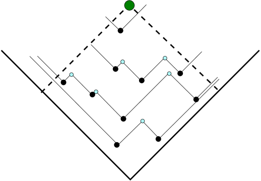
Figure 8: Points of Poisson process (in black), broken lines joining them and points of the second generation (in light blue). Maximum number of points collected along monotonous paths joining points $(\theta,\theta)$ (the big green point) and $(0,0)$ coincides with number of broken lines separating them, which is $4$ in our case. Only the points inside dashed square matter.

We start from the Poisson process in the first quadrant, as in Theorem 1.3 and Figure 5, but now we rotate the quadrant by 45 degrees, like in Figure 4. There is a graphical way to find the value of $L(\theta)$. Namely, for each point of the process draw two rays starting from it and parallel to the axes. Extend each ray till the first intersection with another ray. In this way, we get a collection of broken lines, as shown in Figure 8. At the first intersection points of the rays we put new points that form the second generation. Note now that $L(\theta)$ is equal to the number of broken lines separating $(\theta,\theta)$ and the origin. As it turns out, it is beneficial to iterate this process. We erase all the points of the original Poisson process, but keep the points of the second generation and draw broken lines joining them; we repeat this until no points inside the square with vertices $(0,0)$, $(0,\theta)$, $(\theta,0)$, and $(\theta,\theta)$ are left, as shown in Figure 9. Compute the number of broken lines separating $(\theta,\theta)$ and $(0,0)$ at each step and record these numbers to form a Young diagram $\lambda(\theta)=(\lambda_{1}(\theta),\lambda_{2}(\theta),\dots)$, so that, in particular, $\lambda_{1}(\theta)=L(\theta)$. Observe that $|\lambda(\theta)|$ equals the number of points of the original Poisson process inside the square with vertices $(0,0)$, $(0,\theta)$, $(\theta,0)$, and $(\theta,\theta)$. The procedure we just described is known as Viennot’s geometric construction of the Robinson–Schensted correspondence, see e.g. [Sagan-01].

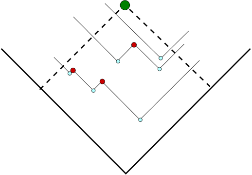
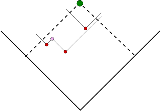
Figure 9: Left panel: Points of second generation (in light blue), broken lines joining them and points of the third generation (in dark red). Right panel: Points of the third generation (in dark red), broken lines joining them and points of the fourth generation (in purple).

Our interest in this construction is based on the fact that the distribution of $\lambda(\theta)$ can be fairly easily computed, as opposed to that of $L(\theta)=\lambda_{1}(\theta)$.

Theorem 4.1.

The distribution of $\lambda(\theta)$ is given by the Poissonized Plancherel measure

$$\mathbb{P}(\lambda(\theta)=\mu)=e^{-\theta^{2}}\left(\frac{\theta^{|\mu|}{\rm dim}(\mu)}{|\mu|!}\right)^{2},\quad\mu\in\mathbb{Y}.$$ (4.1)

Sketch of the proof.

Note that $\lambda(\theta)$ depends only on the relative order of coordinates of the points inside the square with vertices $(0,0)$, $(\theta,0)$, $(0,\theta)$, $(\theta,\theta)$, but not on their positions. This order can be encoded by a permutation $\sigma(\theta)$ which is the permutation between the points ordered by $x$ coordinate and by $y$ coordinate. Observe that the size $n(\theta)$ of $\sigma(\theta)$, i.e. the number of points inside the square, has Poisson distribution with parameter $\theta^{2}$, and given this number, the distribution of $\sigma(\theta)$ is uniform.

Next, we need to use the Robinson-Schensted-Knuth (RSK) correspondence (or rather its earlier Robinson–Schensted version), which is an explicit bijection between permutations of size $n$ and pairs of standard Young tableaux of same shape. We refer the reader to [Sagan-01], [Fulton-97], [Knuth-73] for the definition and properties of this correspondence. What is important for us is that $\lambda(\theta)$ is precisely the common shape of two obtained tableau. Therefore, given that the size $n(\theta)$ of $\sigma(\theta)$ is $m$, the number of boxes in $\lambda(\theta)$ is also $m$, and the conditional distribution of $\lambda(\theta)$ is

$$\mathbb{P}(\lambda(\theta)=\mu\mid n(\theta)=m)=\frac{{\rm dim}^{2}(\mu)}{m!}.$$

Taking into account the Poisson distribution on $m$, we arrive at (4.1). ∎

Remark. The fact that the RSK correspondence is a bijection implies that

$$\sum_{|\lambda|=n}{\rm dim}^{2}(\lambda)=n!.$$ (4.2)

On the other hand, if we recall the definition of ${\rm dim}(\lambda)$ as the dimension of irreducible representation of the symmetric group $S(n)$, then, taking into the account that $|S(n)|=n!$, the equality (4.2) is nothing else but the celebrated Burnside identity which says that squares of the dimensions of irreducible complex representations of any finite group sum up to the number of the elements in the group.

Let us now suggest some intuition on why the asymptotic behavior of $L(\theta)$ should be related to those of growth models and, in particular, to the ballistic deposition that we started with in Section 1. Introduce coordinates $(z,t)$ in Figure 8 so that $t$ is the vertical coordinate, and consider the following growth model. At time $t$ the height profile is given by an integer–valued (random) function $h(x,t)$, at time zero $h(x,0)\equiv 0$. At any given time $t$ and any point $x$, the left and right $x$–limits of the function $h(x,t)$ differ at most by $1$, in other words, $h(x,t)$ is almost surely a step function with steps $(+1)$ (‘‘up step’’, when we read the values of the function from left to right) and $(-1)$ (‘‘down step’’). If there is a point of the Poisson process (of Figure 8) at $(z,t)$, then at time $t$ a seed is born at position $x=z$, which is combination of up and down steps, i.e. $h(z,t)$ increases by $1$. After that the down step starts moving with speed $1$ to the right, while the up step starts moving to the left with the same speed. When the next seed is born, another up and down steps appear and also start moving. When up and down steps (born by different seeds) meet each other, they disappear. This model is known as Polynuclear Growth (PNG), see [Meakin-98], [Prähofer-Spohn-00], a very nice computer simulation for it is available at Ferrari’s website [Ferrari], and at Figure 10 we show one possible height function.

Figure 10: Height function of PNG model after the birth of 3 seeds.

Coming back to Figure 8, note that its broken lines symbolize the space–time trajectories of up/down steps, while second generation points are identified with collisions of up and down steps. In particular, the positions of up and down steps at time $t=t_{0}$ are the points of intersection of the line $t=t_{0}$ at Figure 8 with parts of broken lines of slope $(-1)$ and $(+1)$, respectively. Now it is easy to prove that the PNG-height $h(0,t)$ at time $t$ and point $0$ is precisely the Last Passage Percolation Time $L(t)$. In order to observe the full Young diagram $\lambda(\theta)$ one should introduce multi-layer PNG model, where a seed on level $k$, $k\geq 2$, is born when the up and down steps collide at level $k-1$, and the position of seed coincides with the position of collision, see [Prähofer-Spohn-02] for details.

The PNG model is in the KPZ universality class, and obtaining information on its asymptotic behavior (roughness of interface, fluctuation distributions) would give us similar (although conjectural) statements for other members of the same universality class.

5 The Schur measures and their asymptotic behavior

The aim of this section is to show how the asymptotic behavior of the Poissonized Plancherel measure and certain more general distributions on Young diagrams can be analyzed.

Take any two Schur–positive specializations $\rho_{1}$, $\rho_{2}$ of the algebra of symmetric functions $\Lambda$ (those were classified in Theorem 2.11). The following definition first appeared in [Okounkov-01].

Definition 5.1.

The Schur measure $\mathbb{S}_{\rho_{1};\rho_{2}}$ is a probability measure on the set of all Young diagrams defined through

$$\mathbb{P}_{\rho_{1},\rho_{2}}(\lambda)=\dfrac{s_{\lambda}(\rho_{1})s_{\lambda}(\rho_{2})}{H(\rho_{1};\rho_{2})},$$

where the normalizing constant $H(\rho_{1};\rho_{2})$ is given by

$$H(\rho_{1};\rho_{2})=\exp\left(\sum_{k=1}^{\infty}\frac{p_{k}(\rho_{1})p_{k}(\rho_{2})}{k}\right).$$

Remark. The above definition makes sense only if $\rho_{1}$, $\rho_{2}$ are such that

$$\sum_{\lambda}s_{\lambda}(\rho_{1})s_{\lambda}(\rho_{2})<\infty,$$ (5.1)

and in the latter case this sum equals $H(\rho_{1};\rho_{2})$, as follows from Theorem 2.5. The convergence of (5.1) is guaranteed, for instance, if $|p_{k}(\rho_{1})|<Cr^{k}$ and $|p_{k}(\rho_{2})|<Cr^{k}$ with some constants $C>0$ and $0<r<1$. In what follows we assume that this (or a similar) condition is always satisfied.

Proposition 5.2.

Let $\rho_{\theta}$ be the (Schur–positive) specialization with single non-zero parameter $\gamma=\theta$, i.e.

$$p_{1}(\rho_{\theta})=\theta,\quad p_{k}(\rho_{\theta})=0,\quad k>1.$$

Then $\mathbb{P}_{\rho_{\theta},\rho_{\theta}}$ is the Poissonized Plancherel measure (4.1).

Proof.

This is an immediate corollary of Proposition 2.15. ∎

Our next goal is to show that any Schur measure is a determinantal point process. Given a Young diagram $\lambda$, we associate to it a point configuration $X(\lambda)=\{\lambda_{i}-i+1/2\}\subset\mathbb{Z}+1/2$. This is similar to the correspondence shown in Figures 2, 3. Note that $X(\lambda)$ is semi–infinite, i.e. there are finitely many points to the right of the origin, but almost all points to the left of the origin belong to $X(\lambda)$.

Theorem 5.3 ([Okounkov-01]).

Suppose that the $\lambda\in\mathbb{Y}$ is distributed according to the Schur measure $\mathbb{S}_{\rho_{1};\rho_{2}}$. Then $X(\lambda)$ is a determinantal point process on $\mathbb{Z}+1/2$ with correlation kernel $K(i,j)$ defined by the generating series

$$\sum_{i,j\in\mathbb{Z}+\frac{1}{2}}K(i,j)v^{i}w^{-j}=\frac{H(\rho_{1};v)H(\rho_{2};w^{-1})}{H(\rho_{2};v^{-1})H(\rho_{1};w)}\sum_{k=\frac{1}{2},\frac{3}{2},\frac{5}{2},\dots}\left(\frac{w}{v}\right)^{k},$$ (5.2)

where

$$H(\rho;z)=\sum_{k=0}^{\infty}h_{k}(\rho)z^{k}=\exp\left(\sum_{k=1}^{\infty}p_{k}(\rho)\frac{z^{k}}{k}\right).$$

Remark 1. If we expand $H$–functions in the right–hand side of (5.2) into power series and multiply the resulting expressions, then (5.2) can be viewed as a formal identity of power series.

Remark 2. There is also an analytical point of view on (5.2). Using the fact that (under suitable convergence conditions) the contour integral around zero

$$\frac{1}{2\pi{\mathbf{i}}}\oint\left(\sum_{k=-\infty}^{\infty}a_{k}z^{k}\right)\frac{dz}{z^{n+1}}$$

is equal to $a_{n}$ and also that when $|w|<|v|$ we have

$$\sum_{k=\frac{1}{2},\frac{3}{2},\frac{5}{2},\dots}\left(\frac{w}{v}\right)^{k}=\frac{\sqrt{vw}}{v-w},$$

we can rewrite (5.2) as

$$K(i,j)=\frac{1}{(2\pi{\mathbf{i}})^{2}}\oint\oint\frac{H(\rho_{1};v)H(\rho_{2};w^{-1})}{H(\rho_{2};v^{-1})H(\rho_{1};w)}\frac{\sqrt{vw}}{v-w}\frac{dvdw}{v^{i+1}w^{-j+1}},$$ (5.3)

with integration going over two circles around the origin $|w|=R_{1}$, $|v|=R_{2}$ such that $R_{1}<R_{2}$ and the functions $H(\rho_{1};u)$, $H(\rho_{2};u^{-1})$ are holomorphic in the annulus $R_{1}-\varepsilon<|u|<R_{2}+\varepsilon$. In particular, if $|p_{k}(\rho_{1})|<Cr^{k}$ and $|p_{k}(\rho_{2})|<Cr^{k}$ with some constants $C>0$ and $0<r<1$, then any $r<R_{1}<R_{2}<r^{-1}$ are suitable.

We now present a proof of Theorem 5.3 which is due to Johansson [Johansson-01b], see also [Okounkov-01] for the original proof.

Proof of Theorem 5.3.

We have to prove that for any finite set $A=\{a_{1},\dots,a_{m}\}\subset\mathbb{Z}+1/2$ we have

$$\sum_{\lambda:A\subset X(\lambda)}\dfrac{s_{\lambda}(\rho_{1})s_{\lambda}(\rho_{2})}{H(\rho_{1};\rho_{2})}=\det\left[K(a_{i},a_{j})\right]_{i,j=1}^{m}.$$

For this it suffices to prove the following formal identity of power series. Let $x=(x_{1},\dots)$ and $y=(y_{1},\dots)$ be two sets of variables; then

$$\sum_{\lambda:A\subset X(\lambda)}\dfrac{s_{\lambda}(x)s_{\lambda}(y)}{\prod_{i<j}(1-x_{i}y_{j})^{-1}}=\det\left[\widehat{K}(a_{i},a_{j})\right]_{i,j=1}^{m},$$ (5.4)

where the generating function of $\widehat{K}(i,j)$ is similar to that of $K(i,j)$ but with $\rho_{1}$ and $\rho_{2}$ replaced by $x$ and $y$, respectively. One shows (we omit a justification here) that it is enough to prove (5.4) for arbitrary finite sets of variables $x$ and $y$, so let us prove it for $x=(x_{1},\dots,x_{N})$, $y=(y_{1},\dots,y_{N})$. In the latter case the Schur functions $s_{\lambda}(x)$ are non-zero only if $\ell(\lambda)\leq N$. Because of that it is more convenient to work with a finite point configuration $X_{N}(\lambda)=\{\lambda_{j}+N-j\}_{j=1}^{N}\subset{\mathbb{Z}}_{\geq 0}$ which differs from $X(\lambda)$ in two ways. First there is a deterministic shift by $N-1/2$, this has an evident effect on the correlation functions. Second, $X(\lambda)$ is infinite, while $X_{N}(\lambda)$ is finite. However, the additional points of $X(\lambda)$ (as compared to those of $X_{N}(\lambda)$) are deterministically located and move away to $-\infty$ and, therefore, they do not affect the correlation functions in the end.

The definition of Schur functions (2.5) implies that

$$\dfrac{s_{\lambda}(x_{1},\dots,x_{N})s_{\lambda}(y_{1},\dots,y_{N})}{\prod_{i<j}(1-x_{i}y_{j})^{-1}}=\frac{1}{Z}\det\left[x_{i}^{\lambda_{j}+N-j}\right]_{i,j=1}^{N}\det\left[y_{i}^{\lambda_{j}+N-j}\right]_{i,j=1}^{N}.$$ (5.5)

Now we recognize a biorthogonal ensemble in the right–hand side of (5.5). Therefore, we can use Theorem 3.9 which yields that $X_{N}(\lambda)$ is a determinantal point process with correlation kernel

$$\widetilde{K}(\ell_{1},\ell_{2})=\sum_{i,j=1}^{N}x_{i}^{\ell_{1}}y_{j}^{\ell_{2}}G_{ij}^{-t},$$

where $G_{ij}^{-t}$ is the inverse–transpose matrix of the $N\times N$ Gram matrix

$$G_{ij}=\sum_{\ell\geq 0}x_{i}^{\ell}y_{j}^{\ell}=\frac{1}{1-x_{i}y_{j}}.$$

We can compute the determinant of $G$, which is

$$\det[G_{ij}]_{i,j=1}^{N}=\det\left[\frac{1}{1-x_{i}y_{j}}\right]_{i,j=1}^{N}=\frac{\prod_{i<j}(x_{i}-x_{j})\prod_{i<j}(y_{i}-y_{j})}{\prod_{i,j=1}^{N}(1-x_{i}y_{j})}.$$ (5.6)

This is known as the Cauchy determinant evaluation. One can prove (5.6) directly, see e.g. [Krattenthaler-99]. Another way is to recall that in the proof of Theorem 3.9 we showed that the determinant of $G$ is the normalization constant of the measure, and we know the normalization constant from the very definition of the Schur measure, i.e. by the Cauchy identity.

By the Cramer’s rule, we have

$$(G^{-t})_{k,\ell}=\frac{(-1)^{k+l}\det[G_{ij}]_{i\neq k,j\neq\ell}}{\det[G_{ij}]_{i,j=1}^{N}}.$$

Using the fact that submatrices of $G_{ij}$ are matrices of the same type and their determinants can be evaluated using (5.6), we get

$$(G^{-t})_{k,\ell}=\dfrac{\prod_{j=1}^{N}(1-x_{j}y_{\ell})(1-x_{k}y_{j})}{(1-x_{k}y_{\ell})\prod_{j\neq k}(x_{k}-x_{j})\prod_{j\neq\ell}(y_{j}-y_{\ell})}.$$

We claim that

$$\widetilde{K}(\ell_{1},\ell_{2})=\sum_{i,j=1}^{N}x_{i}^{\ell_{1}}y_{j}^{\ell_{1}}G_{ij}^{-t}=\frac{1}{(2\pi{\mathbf{i}})^{2}}\oint\oint\prod_{k=1}^{N}\frac{(1-zy_{k})(1-vx_{k})}{(z-x_{k})(v-y_{k})}\frac{z^{\ell_{1}}v^{\ell_{2}}}{1-zv}dzdv,$$ (5.7)

with contours chosen so that they enclose the singularities at $z=x_{k}$ and $v=y_{k}$, but do not enclose the singularity at $zv=1$. Indeed, (5.7) is just the evaluation of the double integral as the sum of the residues. Changing the variables $z=1/w$ and shifting $\ell_{1},\ell_{2}$ by $N-1/2$ in (5.7) we arrive at (5.3). ∎

Applying Theorem 5.3 to the Poissonized Plancherel measure we obtain

Corollary 5.4 ([Borodin-Okounkov-Olshanski-00],[Johansson-01a]).

Suppose that $\lambda$ is a random Young diagram distributed by the Poissonized Plancherel measure. Then the points of $X(\lambda)$ form a determinantal point process on $\mathbb{Z}+\frac{1}{2}$ with correlation kernel

$$K_{\theta}(i,j)=\frac{1}{(2\pi{\mathbf{i}})^{2}}\oint\oint\exp\bigg{(}\theta(v-v^{-1}-w+w^{-1})\bigg{)}\frac{\sqrt{vw}}{v-w}\frac{dvdw}{v^{i+1}w^{-j+1}},$$

with integration over positively oriented simple contours enclosing zero and such that $|w|<|v|$.

Our next aim is to study the behavior of $K_{\theta}(i,j)$ as $\theta\to\infty$. The argument below is due to Okounkov [Okounkov-03], but the results were obtained earlier in [Borodin-Okounkov-Olshanski-00], [Johansson-01a] by different tools. Let us start from the case $i=j$. Then $K(i,i)$ is the density of particles of our point process or, looking at Figure 3, the average local slope of the (rotated) Young diagram. Intuitively, one expects to see some non-trivial behavior when $i$ is of order $\theta$. To see that set $i=u\theta$. Then $K_{\theta}$ transforms into

$$K_{\theta}(u\theta,u\theta)=\frac{1}{(2\pi{\mathbf{i}})^{2}}\oint\oint\exp\bigg{(}\theta(S(v)-S(w))\bigg{)}\frac{\sqrt{vw}}{v-w}\frac{dvdw}{vw},$$ (5.8)

with

$$S(z)=z-z^{-1}-u\ln z.$$

Our next aim is to deform the contours of integration so that $\Re(S(v)-S(w))<0$ on them. (It is ok if $\Re(S(v)-S(w))=0$ at finitely many points.) If we manage to do that, then (5.8) would decay as $\theta\to\infty$. Let us try to do this. First, compute the critical points of $S(z)$, i.e. roots of its derivative

$$S^{\prime}(z)=1+z^{-2}-uz^{-1}.$$

When $|u|<2$ the equation $S^{\prime}(z)=0$ has two complex conjugated roots of absolute value $1$ which we denote $e^{\pm i\phi}$. Here $\phi$ satisfies $2\cos(\phi)=u$. Let us deform the contours so that both of them pass through the critical points and look as shown at Figure 11.

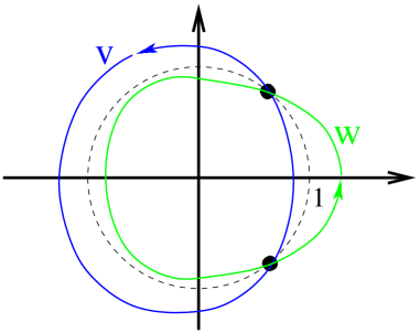
Figure 11: Deformed contours: $v$–contour in blue and $w$–contour in green. The dashed contour is the unit circle and the black dots indicate the critical points of $S(z)$.

We claim that now $\Re S(v)<0$ everywhere on its contour except at critical points $e^{\pm i\phi}$, and $\Re S(w)>0$ everywhere on its contour except at critical points $e^{\pm i\phi}$ ($\Re S(v)=\Re S(w)=0$ at $e^{\pm\phi}$.) To prove that observe that $\Re S(z)=0$ for $z$ on the unit circle $|z|=1$ and compute the gradient of $\Re S(z)=\Re S(a+bi)$ on the unit circle (i.e. when $a^{2}+b^{2}=1$):

$$\Re S(a+bi)=a-\frac{a}{a^{2}+b^{2}}-\frac{u}{2}\ln(a^{2}+b^{2}),$$

$$\nabla\Re S(a+bi)=\left(1-\frac{b^{2}-a^{2}}{(a^{2}+b^{2})^{2}}-\frac{au}{a^{2}+b^{2}}\,,\,\frac{2ab}{(a^{2}+b^{2})^{2}}-\frac{bu}{a^{2}+b^{2}}\right)\\ =\left(1-b^{2}+a^{2}-au\,,2ab-bu\right)=\left(2a^{2}-au\,,2ab-bu\right)=(2a-u)(a,b).$$ (5.9)

Identity (5.9) implies that the gradient vanishes at points $e^{\pm i\phi}$, points outwards the unit circle on the right arc joining the critical points and points inwards on the left arc. This implies our inequalities for $\Re S(z)$ on the contours. (We assume that the contours are fairly close to the unit circle so that the gradient argument works.)

Now it follows that after the deformation of the contours the integral vanishes as $\theta\to\infty$. Does this mean that the correlation functions also vanish? Actually, no. The reason is that the integrand in (5.8) has a singularity at $v=w$. Therefore, when we deform the contours from the contour configuration with $|w|<|v|$, as we had in Corollary 5.4, to the contours of Figure 11 we get a residue of the integrand in (5.8) at $z=w$ along the arc of the unit circle joining $e^{\pm i\phi}$. This residue is

$$\frac{1}{2\pi{\mathbf{i}}}\int_{e^{-i\phi}}^{e^{i\phi}}\frac{dz}{z}=\frac{\phi}{\pi}.$$

We conclude that if $u=2\cos(\phi)$ with $0<\phi<\pi$, then

$$\lim_{\theta\to\infty}K_{\theta}(u\theta,u\theta)=\frac{\phi}{\pi}.$$

Turning to the original picture we see that the asymptotic density of particles at point $i$ changes from $0$ when $i\approx 2\theta$ to $1$ when $i\approx-2\theta$. This means that after rescaling by the factor $\theta^{-1}$ times the Plancherel–random Young diagram asymptotically looks like in Figure 12. This is a manifestation of the Vershik–Kerov–Logan–Shepp limit shape theorem, see [Vershik-Kerov-77], [Logan-Shepp-77].

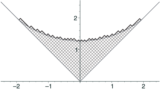
Figure 12: The celebrated Vershik–Kerov–Logan-Shepp curve as a limit shape for the Plancherel random Young diagrams.

More generally, what happens with $K_{\theta}(i,j)$ when $i=u\theta+x$, $j=u\theta+y$ and $\theta\to\infty$? In other words, we want to study how the point configuration (or the boundary of the random Young diagram $\lambda$) behaves in the limit locally near a ‘‘bulk point’’. One proves the following theorem.

Theorem 5.5 ([Borodin-Okounkov-Olshanski-00]).

For any $-2<u<2$ and any two integers $x$, $y$ we have

$$\lim_{\theta\to\infty}K_{\theta}(\lfloor u\theta\rfloor+x,\lfloor u\theta\rfloor+y)=\begin{cases}\dfrac{\sin(\phi(x-y))}{\pi(x-y)},&\text{ if }x\neq y,\\ \dfrac{\phi}{\pi},&\text{ otherwise,}\end{cases}$$ (5.10)

where $\phi=\arccos(u/2)$.

Remark. The right–hand side of (5.10) is known as the discrete sine kernel and it is similar to the continuous sine kernel which arises as a universal local limit of correlation functions for eigenvalues of random Hermitian (Wigner) matrices, see e.g. [Erdos-Yau-12], [Tao-Vu-12] and references therein.

Proof of Theorem 5.5.

The whole argument remains the same as in the case $x=y=0$, except for the computation of the residue which is now

$$\frac{1}{2\pi{\mathbf{i}}}\int_{e^{-i\phi}}^{e^{i\phi}}\frac{dz}{z^{x-y+1}}=\frac{\sin(\phi(x-y))}{\pi(x-y)}.$$ (5.11)

We conclude that if $u=2\cos(\phi)$ with $0<\phi<\pi$, then

$$\lim_{\theta\to\infty}K_{\theta}(\lfloor u\theta\rfloor+x,\lfloor u\theta\rfloor+y)=\frac{\sin(\phi(x-y))}{\pi(x-y)}.$$

∎

So far we got some understanding on what’s happening in the bulk, while we started with the Last Passage Percolation which is related to the so-called edge asymptotic behavior, i.e. limit fluctuations of $\lambda_{1}$. This corresponds to having $u=2$, at which point the above arguments no longer work. With some additional efforts one can prove the following theorem:

Theorem 5.6 ([Borodin-Okounkov-Olshanski-00],[Johansson-01a]).

For any two reals $x$, $y$ we have

$$\lim_{\theta\to\infty}\theta^{1/3}K_{\theta}(2\theta+x\theta^{1/3},2\theta+y\theta^{1/3})=K_{Airy}(x,y)$$ (5.12)

where

$$K_{Airy}(x,y)=\frac{1}{(2\pi{\mathbf{i}})^{2}}\int\int e^{\widetilde{v}^{3}/3-\widetilde{w}^{3}/3+\widetilde{v}x-\widetilde{w}y}\frac{d\widetilde{v}d\widetilde{w}}{\tilde{v}-\tilde{w}},$$ (5.13)

with contours shown at the right panel of Figure 13.

Remark 1. Theorem 5.6 means that the random point process $X(\lambda)$ ‘‘at the edge’’, after shifting by $2\theta$ and rescaling by $\theta^{1/3}$, converges to a certain non-degenerate determinantal random process with state space $\mathbb{R}$ and correlation kernel $K_{Airy}$.

Remark 2. As we will see, Theorem 5.6 implies the following limit theorem for the Last Passage Percolation Time $\lambda_{1}$: For any $s\in\mathbb{R}$

$$\lim_{\theta\to\infty}\mathbb{P}(\lambda_{1}\leq 2\theta+s\theta^{1/3})=\det({\mathbf{1}}-K_{Airy}(x,y))_{L_{2}(s,+\infty)}.$$

One shows that the above Fredholm determinant is the Tracy–Widom distribution $F_{2}(s)$ from Section 1, see [Tracy-Widom-94].

Proof of Theorem 5.6.

We start as in the proof of Theorem 5.5. When $u=2$ the two critical points of $S(z)$ merge, so that the contours now look as in Figure 13 (left panel) and the integral in (5.11) vanishes. Therefore, the correlation functions near the edge tend to $0$. This is caused by the fact that points of our process near the edge rarify, distances between them become large, and the probability of finding a point in any given location tends to $0$.

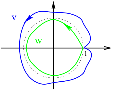
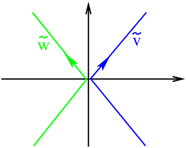
Figure 13: Contours for the edge–scaling limit ($u=2$). Left panel: $v$–contour in blue and $w$–contour in green. The dashed contour is the unit circle. Right panel: limiting contours.

In order to see some nontrivial behavior we need rescaling. Set

$$v=1+\theta^{-1/3}\widetilde{v},\quad w=1+\theta^{-1/3}\widetilde{w}$$

in the contour integral. Note that $z=1$ is a double critical point of $S(z)=z-z^{-1}-2\ln(z)$, so that in the neighborhood of $1$ we have

$$S(z)=\frac{1}{3}(z-1)^{3}+O((z-1)^{4})$$

Now as $\theta\to\infty$ we have

$$\exp\bigg{(}\theta(S(v)-S(w))\bigg{)}=\exp\left(\theta\left(\frac{1}{3}(\theta^{-1/3}\widetilde{v})^{3}-\frac{1}{3}(\theta^{-1/3}\tilde{w})^{3}\right)+o(1)\right)\\ =\exp\left(\frac{1}{3}\widetilde{v}^{3}-\frac{1}{3}\tilde{w}^{3}\right).$$

We conclude that as $\theta\to\infty$

$$K_{\theta}(2\theta+x\theta^{1/3},2\theta+y\theta^{1/3})\approx\frac{\theta^{-1/3}}{(2\pi{\mathbf{i}})^{2}}\int\int e^{\widetilde{v}^{3}/3-\widetilde{w}^{3}/3+\widetilde{v}x-\widetilde{w}y}\frac{d\widetilde{v}d\widetilde{w}}{\tilde{v}-\tilde{w}},$$ (5.14)

and the contours here are contours of Figure 13 (left panel) in the neighborhood of 1; they are shown at the right panel of Figure 13. ∎

Using Theorem 5.6 we can now compute the asymptotic behavior of the Last Passage Percolation time, i.e. of $\lambda_{1}$. Using the inclusion–exclusion principle, for any $A\in\mathbb{R}$ we have

$$\mathbb{P}(\lambda_{1}\leq A)=1-\sum_{x>A}\rho_{1}(x)+\frac{1}{2!}\sum_{x,y>A}\rho_{2}(x,y)-\frac{1}{3!}\sum_{x,y,z>A}\rho_{3}(x,y,z)+\dots$$ (5.15)

Recall that correlation functions $\rho_{k}$ are $k\times k$ determinants involving kernel $K_{\theta}$, substitute $A=2\theta+s\theta^{1/3}$ and send $\theta\to\infty$. The sums in (5.15) turn into the integrals and we get (ignoring convergence issues, which can, however, be handled)

$$\lim_{\theta\to\infty}\mathbb{P}(\lambda_{1}\leq 2\theta+s\theta^{1/3})=1-\int_{x>s}K_{Airy}(x,x)dx\\ +\frac{1}{2!}\int_{x,y>s}\det\begin{bmatrix}K_{Airy}(x,x)&K_{Airy}(x,y)\\ K_{Airy}(y,x)&K_{Airy}(y,y)\end{bmatrix}dxdy-\dots\,.$$

In the last expression one recognizes the Fredholm determinant expansion (see e.g. [Lax-02] or [Simon-05]) for

$$\det({\mathbf{1}}-K_{Airy}(x,y))_{L_{2}(s,+\infty)}.$$

The conceptual conclusion from all the above is that as soon as we have an integral representation for the correlation kernel of a point process, many limiting questions can be answered by analyzing these integrals. The method for the analysis that we presented is, actually, quite standard and is well-known (at least since the $XIX$ century) under the steepest descent method name. In the context of determinantal point processes and Plancherel measures it was pioneered by Okounkov and we recommend [Okounkov-03] for additional details.

6 The Schur processes and Markov chains

While in the previous sections we gave a few of tools for solving the problems of probabilistic origin, in this section we present a general framework, which produces ‘‘analyzable’’ models.

6.1 The Schur process

The following definition is due to [Okounkov-Reshetikhin-01].

Definition 6.1.

The Schur process (of rank $N$) is a probability measure on sequences of Young diagrams $\lambda^{(1)},\mu^{(1)},\lambda^{(2)},\mu^{(2)},\dots,\mu^{(N-1)},\lambda^{(N)}$, parameterized by $2N$ Schur–positive specializations $\rho_{0}^{+},\dots,\rho^{+}_{N-1}$, $\rho_{1}^{-},\dots,\rho_{N}^{-}$ and given by

$$\mathbb{P}\bigg{(}\lambda^{(1)},\mu^{(1)},\lambda^{(2)},\mu^{(2)},\dots,\mu^{(N-1)},\lambda^{(N)}\bigg{)}\\ =\frac{1}{Z}s_{\lambda^{(1)}}(\rho^{+}_{0})s_{\lambda^{(1)}/\mu^{(1)}}(\rho^{-}_{1})s_{\lambda^{(2)}/\mu^{(1)}}(\rho^{+}_{1})\cdots s_{\lambda^{(N)}/\mu^{(N-1)}}(\rho^{+}_{N-1})s_{\lambda^{(N)}}(\rho^{-}_{N}),$$ (6.1)

where $Z$ is a normalization constant.

Proposition 2.8 implies that in Definition 6.1 almost surely

$$\lambda^{(1)}\supset\mu^{(1)}\subset\lambda^{(2)}\supset\dots\supset\mu^{(N-1)}\subset\lambda^{(N)}.$$

It is convenient to use the graphical illustration for the Schur process as shown in Figure 14.

Figure 14: Graphical illustration for the Schur process with $N=3$.

Note that if we set $N=1$ in the definition of the Schur process then we get back the Schur measure of Definition 5.1.

Let us introduce some further notations. For two Schur–positive specializations $\rho$, $\rho^{\prime}$ we set

$$H(\rho;\rho^{\prime})=\exp\left(\sum_{k=1}^{\infty}\frac{p_{k}(\rho)p_{k}(\rho^{\prime})}{k}\right).$$

Given two specializations $\rho_{1},\rho_{2}$, their union $(\rho_{1},\rho_{2})$ is defined through its values on power sums $p_{k}$

$$p_{k}(\rho_{1},\rho_{2})=p_{k}(\rho_{1})+p_{k}(\rho_{2}).$$

Theorem 2.11 implies that if $\rho_{1}$ is a Schur–positive specialization with parameters $(\alpha^{(1)},\beta^{(1)},\gamma^{(1)})$, and $\rho_{2}$ is a Schur–positive specialization with parameters $(\alpha^{(2)},\beta^{(2)},\gamma^{(2)})$, then $(\rho_{1},\rho_{2})$ is a Schur–positive specialization with parameters $(\alpha^{(1)}\bigcup\alpha^{(2)},\beta^{(1)}\bigcup\beta^{(2)},\gamma^{(1)}+\gamma^{(2)})$, where $\alpha^{(1)}\bigcup\alpha^{(2)}$ stands for the sequence obtained by rearranging the union of sequences $\alpha^{(1)}$ and $\alpha^{(2)}$ in decreasing order (and similarly for $\beta$). In particular, if $\rho_{1}$ and $\rho_{2}$ specialize symmetric functions by substituting sets of variables, say $(x_{1},x_{2},\dots)$ and $(y_{1},y_{2},\dots)$ (which corresponds to zero $\beta_{i}$ and $\gamma$), then $(\rho_{1},\rho_{2})$ substitutes all the variables $(x_{1},x_{2},\dots,y_{1},y_{2},\dots)$.

The definition implies that for specializations $\rho_{1},\dots,\rho_{k}$, $\rho^{\prime}_{1},\dots,\rho^{\prime}_{m}$ we have

$$H(\rho_{1},\dots,\rho_{k};\rho^{\prime}_{1},\dots,\rho^{\prime}_{m})=\prod_{i=1}^{k}\prod_{j=1}^{m}H(\rho_{i};\rho_{j}).$$

Proposition 6.2.

Suppose that for every $i<j$ we have $H(\rho_{i}^{+};\rho_{j}^{-})<\infty$. Then the Schur process is well–defined and the normalization constant $Z$ in its definition is

$$Z=\prod_{i<j}H(\rho_{i}^{+};\rho_{j}^{-}).$$

Proof.

The proof is based on the iterated applications of identities

$$\sum_{\mu\in\mathbb{Y}}s_{\mu/\lambda}(\rho)s_{\mu/\nu}(\rho^{\prime})\\ =H(\rho;\rho^{\prime})\sum_{\kappa\in\mathbb{Y}}s_{\lambda/\kappa}(\rho^{\prime})s_{\nu/\kappa}(\rho)$$

and

$$s_{\lambda/\mu}(\rho,\rho^{\prime})=\sum_{\nu\in\mathbb{Y}}s_{\lambda/\nu}(\rho)s_{\nu/\mu}(\rho^{\prime}).$$

The above identities are valid for any specializations $\rho$, $\rho^{\prime}$ such that all the sums are convergent and are just the results of the application of these specializations to the statements of Propositions 2.7 and 2.9.

We have:

$$\sum s_{\lambda^{(1)}}(\rho^{+}_{0})s_{\lambda^{(1)}/\mu^{(1)}}(\rho^{-}_{1})s_{\lambda^{(2)}/\mu^{(1)}}(\rho^{+}_{1})\cdots s_{\lambda^{(N)}/\mu^{(N-1)}}(\rho^{+}_{N})s_{\lambda^{(N)}}(\rho^{-}_{N})\\ =H(\rho^{+}_{0};\rho^{-}_{1})\sum s_{\varnothing/\nu}(\rho^{-}_{1})s_{\mu^{(1)}/\nu}(\rho^{+}_{0})s_{\lambda^{(2)}/\mu^{(1)}}(\rho^{+}_{1})\cdots s_{\lambda^{(N)}/\mu^{(N-1)}}(\rho^{+}_{N})s_{\lambda^{(N)}}(\rho^{-}_{N})\\ =H(\rho^{+}_{0};\rho^{-}_{1})\sum s_{\varnothing/\nu}(\rho^{-}_{1})s_{\lambda^{(2)}/\nu}(\rho^{+}_{0},\rho^{+}_{1})\cdots s_{\lambda^{(N)}/\mu^{(N-1)}}(\rho^{+}_{N})s_{\lambda^{(N)}}(\rho^{-}_{N})\\ =H(\rho^{+}_{0};\rho^{-}_{1})\sum s_{\lambda^{(2)}}(\rho^{+}_{0},\rho^{+}_{1})\cdots s_{\lambda^{(N)}/\mu^{(N-1)}}(\rho^{+}_{N})s_{\lambda^{(N)}}(\rho^{-}_{N}),$$ (6.2)

where we used the fact that $s_{\varnothing/\nu}=0$ unless $\lambda^{(1)}=\varnothing$, and $s_{\varnothing/\varnothing}=1$. Note, that the summation in the last line of (6.2) runs over $\lambda^{(2)},\mu^{(2)},\dots,\mu^{(N-1)},\lambda^{(N)}$, i.e. there is no summation over $\lambda^{(1)},\mu^{(1)}$ anymore. Iterating this procedure, we get the value of the normalization constant $Z$. ∎

It turns out that ‘‘one–dimensional’’ marginals of the Schur processes are the Schur measures:

Proposition 6.3.

The projection of the Schur process to the Young diagram $\lambda^{(k)}$ is the Schur measure $\mathbb{S}_{\rho_{1};\rho_{2}}$ with specializations

$$\rho_{1}=(\rho^{+}_{0},\rho^{+}_{1},\dots,\rho^{+}_{k-1}),\quad\rho_{2}=(\rho^{-}_{k},\rho^{-}_{k+1},\dots,\rho^{-}_{N}).$$

Proof.

The proof is analogous to that of Proposition 6.2. ∎

Proposition 6.3 means that the projection of a Schur process to the Young diagram $\lambda^{(k)}$ can be identified with a determinantal point process and, thus, can be analyzed with methods of Section 5. In fact, a more general statement is true: The joint distribution of all Young diagrams of a Schur process is also a determinantal point process with correlation kernel similar to that of Theorem 5.3, see [Okounkov-Reshetikhin-01], [Borodin-Rains-05].

Note that if one of the specializations, say $\rho^{+}_{k}$ is trivial, i.e. this is the Schur positive specialization $(0;0;0)$, then (since $s_{\lambda/\mu}(0;0;0)=0$ unless $\lambda=\mu$) two of the Young diagrams should coincide, namely $\mu^{(k)}=\lambda^{(k+1)}$. In this case we can safely forget about $\mu^{(k)}$ and omit it from our notations. This also shows that in the definition of the Schur process we could replace the saw–like diagram of Figure 14 by any staircase–like scenario.

Let us give two examples of the Schur processes.

6.2 Example 1. Plane partitions

A plane partition $Y$ is a $2d$ array of non-negative integers $Y_{ij}$, $i,j=1,2,\dots$, such that $\sum_{i,j}Y_{ij}<\infty$ and the numbers weakly decrease along the rows and columns, i.e. if $i^{\prime}\geq i$ and $j^{\prime}\geq j$, then $Y_{ij}\geq Y_{i^{\prime}j^{\prime}}$. The sum $\sum_{i,j}Y_{ij}$ is called the volume of the plane partition $Y$. In the same way as ordinary partitions were identified with Young diagrams in Section 2, plane partitions can be identified with $3d$ Young diagrams. To see that, view a plane partition as a collection of numbers written in the vertices of the regular square grid on the plane and put $k$ unit cubes on each number $k$. The resulting $3d$ body is the desired $3d$ Young diagram; an example is shown in Figure 15.

Figure 15: Left panel: Plane partition of volume $5$. Right panel: The corresponding $3d$ Young diagram.

Fix $q$, $0<q<1$ and consider the following probability measure on the set of all plane partitions

$$\mathbb{P}(Y)=\frac{1}{M}q^{{\rm volume}(Y)},$$

which is one of the simplest (speaking of definition, not properties) possible probability measures on this set. The normalization constant $M$ is given by the celebrated MacMahon formula (see [MacMahon-1912], [Stanley-99, Section 7.20], [Macdonald-95, Chapter I, Section 5, Example 13])

$$M=\prod_{n=1}^{\infty}(1-q^{n})^{-n}.$$

We claim that the above measure can be described via a Schur process. In fact this is a particular case of a more general statement that we now present.

Definition 6.4.

Fix two natural numbers $A$ and $B$. For a Young diagram $\pi\subset B^{A}=(\underbrace{B,\dots,B}_{A\text{ times}})$, set $\bar{\pi}=B^{A}/\pi$. A skew plane partition $\Pi$ with support $\bar{\pi}$ is a filling of all boxes of $\bar{\pi}$ by nonnegative integers $\Pi_{i,j}$ (we assume that $\Pi_{i,j}$ is located in the $i$th row and $j$th column of $B^{A}$) such that $\Pi_{i,j}\geq\Pi_{i,j+1}$ and $\Pi_{i,j}\geq\Pi_{i+1,j}$ for all values of $i,j$. The volume of the skew plane partition $\Pi$ is defined as

$${\rm volume}(\Pi)=\sum_{i,j}\Pi_{i,j}.$$

For an example of a skew plane partition see Figure 16.

Our goal is to explain that the measure on plane partitions with given support $\bar{\pi}$ and weights proportional to $q^{{\rm volume}(\,\cdot\,)}$, $0<q<1$, is a Schur process. This fact has been observed and used in [Okounkov-Reshetikhin-01], [Okounkov-Reshetikhin-05], [Okounkov-Reshetikhin-06], [Boutillier-Mkrtchyan-Reshetikhin-Tingley-12], [Borodin-11].

The Schur process will be such that for any two neighboring specializations $\rho_{k}^{-},\rho_{k}^{+}$ at least one is trivial. This implies that each $\mu^{(j)}$ coincides either with $\lambda^{(j)}$ or with $\lambda^{(j+1)}$. Thus, we can restrict our attention to $\lambda^{(j)}$’s only.

For a plane partition $\Pi$, we define the Young diagrams $\lambda^{(k)}$ ($1\leq k\leq A+B+1$) via

$$\lambda^{(k)}(\Pi)=\bigl{\{}\Pi_{i,i+k-A-1}\mid(i,i+k-A-1)\in\bar{\pi}\bigr{\}}.$$

Note that $\lambda^{(1)}=\lambda^{(A+B+1)}=\varnothing$. Figure 16 shows a skew plane partition $\Pi$ and corresponding sequence of Young diagrams.

Figure 16: A skew plane partition $\Pi$ with support $B^{A}/\pi$. Here $B=A=4$ and $\pi=(2,1,1)$. The corresponding sequence of Young diagrams is $\varnothing\subset(6)\supset(5)\subset(8,4)\subset(10,5,3)\supset(7,3)\subset(9,6)\supset(8)\supset\varnothing.$

We need one more piece of notation. Define

$${\mathcal{L}}(\pi)=\{A+\pi_{i}-i+1\mid i=1,\dots,A\}.$$

This is an $A$-point subset in $\{1,2,\dots,A+B\}$, and all such subsets are in bijection with the partitions $\pi$ contained in the box $B^{A}$; this is similar to the identification of Young diagrams and point configurations used in Theorem 5.3. The elements of ${\mathcal{L}}(\pi)$ mark the up-right steps in the boundary of $\pi$ (=back wall of $\Pi$), as in Figure 16.

Theorem 6.5.

Let $\pi$ be a partition contained in the box $B^{A}$. The measure on the plane partitions $\Pi$ with support $\bar{\pi}$ and weights proportional to $q^{vol(\Pi)}$, is the Schur process with $N=A+B+1$ and Schur–positive specializations $\{\rho_{i}^{+}\}$, $\{\rho_{j}^{-}\}$ defined by

$$\rho_{0}^{+}=\rho_{N}^{-}=(0;0;0)$$ (6.3)

$$\rho_{j}^{+}=\begin{cases}(q^{-j};0;0),&j\in{\mathcal{L}}(\pi),\\ (0;0;0),&j\notin{\mathcal{L}}(\pi);\end{cases}\qquad\rho_{j}^{-}=\begin{cases}(0;0;0),&j\in{\mathcal{L}}(\pi),\\ (q^{j};0;0),&j\notin{\mathcal{L}}(\pi),\end{cases}$$ (6.4)

where $(a;0;0)$ is the Schur–positive specialization with single non-zero parameter $\alpha_{1}=a$.

Remark. One can send $A,B$ to infinity in Theorem (6.5). If $\pi=\varnothing$, then we get plane partitions ($3d$ Young diagrams) we started with.

Proof of Theorem 6.5.

Definition 6.4 and Proposition 2.12 imply that the set of all skew plane partitions supported by $\bar{\pi}$, as well as the support of the Schur process from the statement of the theorem, consists of sequences $(\lambda^{(1)},\lambda^{(2)},\dots,\lambda^{(N)})$ with

$$\begin{gathered}\lambda^{(1)}=\lambda^{(N)}=\varnothing,\\ \lambda^{(j)}\prec\lambda^{(j+1)}\text{ if }j\in{\mathcal{L}}(\lambda),\qquad\lambda^{(j)}\succ\lambda^{(j+1)}\text{ if }j\notin{\mathcal{L}}(\lambda),\end{gathered}$$

where we write $\mu\prec\nu$ or $\nu\succ\mu$ if $\nu_{1}\geq\mu_{1}\geq\nu_{2}\geq\mu_{2}\geq\dots$ .

On the other hand, Proposition 2.12 implies that the weight of $(\lambda^{(1)},\lambda^{(2)},\dots,\lambda^{(N)})$ with respect to the Schur process from the hypothesis is equal to $q$ raised to the power

$$\sum_{j=2}^{A+B}\left|\lambda^{(j)}\right|\Bigl{(}-(j-1){\mathbb{1}}_{j-1\in{\mathcal{L}}(\pi)}-(j-1){\mathbb{1}}_{j-1\notin{\mathcal{L}}(\pi)}+j{\mathbb{1}}_{j\in{\mathcal{L}}(\pi)}+j{\mathbb{1}}_{j\notin{\mathcal{L}}(\pi)}\Bigr{)},$$

where the four terms are the contributions of $\rho_{j-1}^{+},\rho_{j-1}^{-},\rho_{j}^{+},\rho_{j}^{-}$, respectively.

Clearly, the sum is equal to $\sum_{j=2}^{A+B}|\lambda^{(j)}|={\rm volume}(\Pi)$. ∎

Theorem 6.5 gives a way for analyzing random (skew) plane partitions via the approach of Section 5. Using this machinery one can prove various interesting limit theorems describing the asymptotic behavior of the model as $q\to 1$, see [Okounkov-Reshetikhin-01], [Okounkov-Reshetikhin-05], [Okounkov-Reshetikhin-06], [Boutillier-Mkrtchyan-Reshetikhin-Tingley-12].

6.3 Example 2. RSK and random words

Our next example is based on the Robinson–Schensted–Knuth correspondence and is a generalization of constructions of Section 4.

Take the alphabet of $N$ letters $\{1,\dots,N\}$ and a collection of positive parameters $a_{1},\dots,a_{N}$. Consider a growth process of the random word $\omega_{N}(t)$ with each letter $j$ appearing (independently) at the end of the word according to a Poisson process of rate $a_{j}$. In particular, the length $|\omega_{N}(t)|$ of the word at time $t$ is a Poisson random variable with parameter $(a_{1}+\dots+a_{N})t$:

$$\mathbb{P}(|\omega_{N}(t)|=k)=e^{-(a_{1}+\dots+a_{N})t}\frac{((a_{1}+\dots+a_{N})t)^{k}}{k!}.$$

The growth of $\omega_{N}(t)$ can be illustrated by the random point process with point $(t,j)$ appearing if the letter $j$ is added to the word at time $t$, see Figure 17. For any $T>0$, one can produce a Young diagram $\lambda^{(N)}(T)$ from all the points $(t,j)$ with $t\leq T$ using the Robinson–Schensted-Knuth (RSK) algorithm, whose geometric version was given in Section 4. (We again address the reader to [Sagan-01], [Fulton-97], [Knuth-73] for the details on RSK.) In particular, the length of the first row of $\lambda^{(N)}(T)$ equals the maximal number of points one can collect along a monotonous path joining $(0,0)$ and $(T,N)$, as in Figure 17. More generally, let $w_{N-k}(t)$ be the word obtained from $w_{N}(t)$ by removing all the instances of letters $N,N-1,\dots,N-k+1$, and let $\lambda^{(N-k)}(T)$ denote the Young diagram corresponding to $w_{N-k}(t)$, i.e. this is the Young diagram obtained from all the points $(t,j)$ with $t\leq T$, $j\leq N-k$.

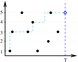
Figure 17: Collection of points with coordinates $(t,j)$ corresponding to the growth of random word and the path collecting maximal number of points $\ell_{N}(T)=\lambda^{(N)}(T)=5$. Here $N=5$.

Proposition 6.6.

For any $t$ and $N$ the collection of (random) Young diagrams $\lambda^{(1)}(t),\lambda^{(2)}(t),\dots,\lambda^{(N)}(t)$ forms a Schur process with probability distribution

$$\frac{1}{Z}s_{\lambda^{(1)}}(a_{1})s_{\lambda^{(2)}/\lambda^{(1)}}(a_{2})\cdots s_{\lambda^{(N)}/\lambda^{(N-1)}}(a_{N})s_{\lambda(N)}(\rho_{t}),$$

where we identify $a_{i}$ with the Schur–positive specialization with parameter $\alpha_{1}=a_{i}$ and all other parameters $0$, and $\rho_{t}$ is the specialization with single non-zero parameter $\gamma=t$.

Proof.

This statement follows from properties of RSK correspondence, cf. [Johansson-05]. ∎

Now let us concentrate on the random vector $(\ell_{1}(t),\dots,\ell_{N}(t))=(\lambda^{(1)}_{1}(t),\dots,\lambda_{1}^{(N)}(t))$ and try to describe its time evolution as $t$ grows. Recall that in Figure 17 the value of $\ell_{k}(T)$ is the maximal number of points collected along monotonous paths joining $(0,0)$ and $(T,k)$. Suppose that at time $t$ a new letter $k$ appears, so that there is a point $(t,k)$ in the picture. It means that $\ell_{k}$ grows by $1$ ($\ell_{k}(t)=\ell_{k}(t-)+1$), because we can add this point to any path coming to any $(t^{\prime},k)$ with $t^{\prime}<k$. Clearly, $\ell_{j}$ does not change for $j<k$. Note that if $\ell_{k+1}(t-)>\ell_{k}(t-)$, then $\ell_{k+1}$ also does not change, since the maximal number of points collected along a path passing through $(t,k)$ is at most $\ell_{k}(t)$. Finally, if $\ell_{k}(t-)=\ell_{k+1}(t-)=\dots=\ell_{k+m}(t-)$, then all the numbers $\ell_{k},\dots,\ell_{k+m}$ should increase by $1$, since the optimal path will now go through $(t,k)$ and collect $\ell_{k}$ points.

The above discussion shows that the evolution of $(\ell_{1}(t),\dots,\ell_{N}(t))$ is a Markov process, and it admits the following interpretation. Take $N$ (distinct) particles on $\mathbb{Z}$ with coordinates $\ell_{1}+1<\ell_{2}+2<\dots<\ell_{N}+N$. Each particle has an independent exponential clock of rate $a_{i}$. When a clock rings, the corresponding particle attempts to jump to the right by one. If that spot is empty then the particle jumps and nothing else happens. Otherwise, in addition to the jump, the particle pushes all immediately right adjacent particles by one, see Figure 18 for an illustration of these rules. The dynamics we have just described is known as the Long Range Totally Asymmetric Exclusion Process, and it is also a special case of PushASEP, see [Borodin-Ferrari-08a], [Spitzer-70].

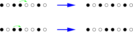
Figure 18: PushASEP. Top panel: jump of a particle. Bottom panel: jump of a particle which results in pushing.

We also note (without proof) that if instead of $(\lambda^{(1)}_{1}(t),\dots,\lambda_{1}^{(N)}(t))$ one considers the random vector $(\lambda^{(1)}_{1}(t),\lambda^{(2)}_{2}(t)\dots,\lambda_{N}^{(N)}(t))$, then the fixed time distribution of the particles $\lambda_{N}^{(N)}-N<\lambda_{N-1}^{(N-1)}-(N-1)<\dots<\lambda_{1}^{(1)}-1$ coincides with that of the well-known TASEP process that was presented in Section 1.

The conclusion now is that Proposition 6.6 together with methods of Section 5 gives a way of the asymptotic analysis of TASEP and PushASEP stochastic dynamics at large times. In particular, one can prove the analogues of Theorems 1.3, 1.4, 1.5, see e.g. [Johansson-00], [Borodin-Ferrari-08a].

6.4 Markov chains on Schur processes

In the last section we linked Schur processes to simple particle dynamics like TASEP using the RSK correspondence. In this section we produce another family of Markov dynamics connecting such objects whose description is arguably more straightforward and independent of complicated combinatorial algorithms, such as RSK.

We start by introducing a general framework. Let $\rho$ and $\rho^{\prime}$ be two Schur–positive specializations such that $H(\rho;\rho^{\prime})<\infty$. Define matrices $p^{\uparrow}_{\lambda\to\mu}$ and $p^{\downarrow}_{\lambda\to\mu}$ with rows and columns indexed by Young diagrams $\lambda$ and $\mu$ as follows:

$$p^{\uparrow}_{\lambda\to\mu}(\rho;\rho^{\prime})=\frac{1}{H(\rho;\rho^{\prime})}\frac{s_{\mu}(\rho)}{s_{\lambda}(\rho)}s_{\mu/\lambda}(\rho^{\prime}),$$ (6.5)

$$p^{\downarrow}_{\lambda\to\mu}(\rho;\rho^{\prime})=\frac{s_{\mu}(\rho)}{s_{\lambda}(\rho,\rho^{\prime})}s_{\lambda/\mu}(\rho^{\prime}).$$ (6.6)

Proposition 6.7.

The matrices $p^{\uparrow}_{\lambda\to\mu}$ and $p^{\downarrow}_{\lambda\to\mu}$ are stochastic, i.e. all matrix elements are non-negative, and for every $\lambda\in\mathbb{Y}$ we have

$$\sum_{\mu\in\mathbb{Y}}p^{\uparrow}_{\lambda\to\mu}(\rho,\rho^{\prime})=1,$$ (6.7)

$$\sum_{\mu\in\mathbb{Y}}p^{\downarrow}_{\lambda\to\mu}(\rho,\rho^{\prime})=1.$$ (6.8)

Proof.

Non-negativity of matrix elements follows from the definition of Schur–positive specializations. Equality (6.7) is a specialized version of the skew Cauchy identity of Proposition 2.7, and equality (6.8) is a specialized version of Proposition 2.9. ∎

Proposition 6.7 means that matrices $p^{\uparrow}_{\lambda\to\mu}$ and $p^{\downarrow}_{\lambda\to\mu}$ can be viewed as transitional probabilities of Markov chains. Definitions (6.5), (6.6) and Proposition 2.8 imply that $p^{\uparrow}_{\lambda\to\mu}=0$ unless $\mu\supset\lambda$, i.e. the Young diagram increases, and $p^{\downarrow}_{\lambda\to\mu}=0$ unless $\mu\subset\lambda$, i.e. the Young diagram decreases (hence up and down arrows in the notations).

One of the important properties of the above stochastic matrices is that they agree with Schur measures, i.e. Markov chains defined using them preserve the class of Schur measures. Formally, we have the following statement:

Proposition 6.8.

For any $\mu\in\mathbb{Y}$ we have

$$\sum_{\lambda\in\mathbb{Y}}{\mathbb{S}}_{\rho_{1};\rho_{2}}(\lambda)p^{\uparrow}_{\lambda\to\mu}(\rho_{2};\rho_{3})={\mathbb{S}}_{\rho_{1},\rho_{3};\rho_{2}}(\mu)$$

and

$$\sum_{\lambda\in\mathbb{Y}}{\mathbb{S}}_{\rho_{1};\rho_{2},\rho_{3}}(\lambda)p^{\downarrow}_{\lambda\to\mu}(\rho_{2};\rho_{3})={\mathbb{S}}_{\rho_{1};\rho_{2}}(\mu).$$

Remark. Informally, $p^{\uparrow}_{\lambda\to\mu}$ increases the specialization by adding $\rho_{3}$, while $p^{\downarrow}_{\lambda\to\mu}$ decreases the specialization by removing $\rho_{3}$. Note also that ${\mathbb{S}}_{\rho_{1};\rho_{2}}={\mathbb{S}}_{\rho_{2};\rho_{1}}$ for any $\rho_{1},\rho_{2}$.

Proof of Proposition 6.8.

This is an application of the specialized versions of Propositions 2.7 and 2.9. ∎

Next, note that the distribution of the Schur process of the form which appeared in Proposition 6.6

$$\frac{1}{Z}s_{\lambda^{(1)}}(\rho^{+}_{0})s_{\lambda^{(2)}/\lambda^{(1)}}(\rho^{+}_{1})\cdots s_{\lambda^{(N)}/\lambda^{(N-1)}}(\rho^{+}_{N-1})s_{\lambda(N)}(\rho_{-})$$

can be rewritten as

$${\mathbb{S}}_{\rho^{+}_{0},\dots,\rho^{+}_{N-1};\rho^{-}}(\lambda^{(N)})p^{\downarrow}_{\lambda^{(N)}\to\lambda^{(N-1)}}(\rho^{+}_{0},\dots,\rho^{+}_{N-2};\rho^{+}_{N-1})\cdots p^{\downarrow}_{\lambda^{(2)}\to\lambda^{(1)}}(\rho^{+}_{0};\rho^{+}_{1}).$$

More generally, any Schur process can be viewed as a trajectory of a Markov chain with transitional probabilities given by matrices $p^{\uparrow}$ and $p^{\downarrow}$ (with suitable specializations) and initial distribution being a Schur measure.

Another property that we need is the following commutativity.

Proposition 6.9.

The following commutation relation on matrices $p^{\uparrow}_{\lambda\to\mu}$ and $p^{\downarrow}_{\lambda\to\mu}$ holds:

$$p^{\uparrow}(\rho_{1},\rho_{2};\rho_{3})p^{\downarrow}(\rho_{1};\rho_{2})=p^{\downarrow}(\rho_{1};\rho_{2})p^{\uparrow}(\rho_{1};\rho_{3})$$ (6.9)

Remark. In terms of acting on Schur measures, as in Proposition 6.8, (6.9) says that adding $\rho_{3}$ and then removing $\rho_{2}$ is the same as first removing $\rho_{2}$ and then adding $\rho_{3}$:

$$\begin{array}[]{ll}{\mathbb{S}}_{\rho_{4};\rho_{1},\rho_{2}}p^{\uparrow}(\rho_{1},\rho_{2};\rho_{3})={\mathbb{S}}_{\rho_{3},\rho_{4};\rho_{1},\rho_{2}},&{\mathbb{S}}_{\rho_{3},\rho_{4};\rho_{1},\rho_{2}}p^{\downarrow}(\rho_{1};\rho_{2})={\mathbb{S}}_{\rho_{3},\rho_{4};\rho_{1}},\\ {\mathbb{S}}_{\rho_{4};\rho_{1},\rho_{2}}p^{\downarrow}(\rho_{1};\rho_{2})={\mathbb{S}}_{\rho_{4};\rho_{1}},&{\mathbb{S}}_{\rho_{4};\rho_{1}}p^{\uparrow}(\rho_{1};\rho_{3})={\mathbb{S}}_{\rho_{3},\rho_{4};\rho_{1}}.\end{array}$$

Proof of Proposition 6.9.

We should prove that for any $\lambda,\nu\in\mathbb{Y}$

$$\sum_{\mu\in\mathbb{Y}}p^{\uparrow}_{\lambda\to\mu}(\rho_{1},\rho_{2};\rho_{3})p^{\downarrow}_{\mu\to\nu}(\rho_{1};\rho_{2})=\sum_{\mu\in\mathbb{Y}}p^{\downarrow}_{\lambda\to\mu}(\rho_{1};\rho_{2})p^{\uparrow}_{\mu\to\nu}(\rho_{1};\rho_{3}).$$

Using definitions (6.5), (6.6) this boils down to the specialized version of the skew Cauchy Identity, which is Proposition 2.7, cf. [Borodin-11]. ∎

Commutativity relation (6.9) paves the way to introducing a family of new Markov chains through a construction that we now present. This construction first appeared in [Diaconis-Fill-90] and was heavily used recently for probabilistic models related to Young diagrams, see [Borodin-Ferrari-08b], [Borodin-Gorin-08], [Borodin-Gorin-Rains-10], [Borodin-Duits-11], [Borodin-11], [Borodin-Olshanski-12], [Betea-11], [Borodin-Corwin-11].

Take two Schur–positive specializations $\rho_{1}$, $\rho_{2}$ and a state space $\mathbb{Y}^{(2)}$ of pairs of Young diagrams $\lambda^{(2)}\choose\lambda^{(1)}$ such that $p^{\downarrow}_{\lambda^{(2)}\to\lambda^{(1)}}(\rho_{1};\rho_{2})>0$. Define a Markov chain on $\mathbb{Y}^{(2)}$ with the following transition probabilities:

$$\mathbb{P}\left({\lambda^{(2)}\choose\lambda^{(1)}}\to{\mu^{(2)}\choose\mu^{(1)}}\right)=p^{\uparrow}_{\lambda^{(1)}\to\mu^{(1)}}(\rho_{1};\rho^{\prime})\dfrac{p^{\uparrow}_{\lambda^{(2)}\to\mu^{(2)}}(\rho_{1},\rho_{2};\rho^{\prime})p^{\downarrow}_{\mu^{(2)}\to\mu^{(1)}}(\rho_{1};\rho_{2})}{\sum_{\mu}p^{\uparrow}_{\lambda^{(2)}\to\mu}(\rho_{1},\rho_{2};\rho^{\prime})p^{\downarrow}_{\mu\to\mu^{(1)}}(\rho_{1};\rho_{2})}$$ (6.10)

In words (6.10) means that the first Young diagram $\lambda^{(1)}\to\mu^{(1)}$ evolves according to the transition probabilities $p^{\uparrow}_{\lambda^{(1)}\to\mu^{(1)}}(\rho_{1};\rho^{\prime})$, and given $\lambda^{(2)}$ and $\mu^{(1)}$ the distribution of $\mu^{(2)}$ is the distribution of the middle point in the two-step Markov chain with transitions $p^{\uparrow}_{\lambda^{(2)}\to\mu}(\rho_{1},\rho_{2};\rho^{\prime})$ and $p^{\downarrow}_{\mu\to\mu^{(1)}}(\rho_{1};\rho_{2})$.

Proposition 6.10.

The above transitional probabilities on $\mathbb{Y}^{(2)}$ map the Schur process with distribution

$${\mathbb{S}}_{\rho_{1},\rho_{2};\rho^{-}}(\lambda^{(2)})p^{\downarrow}_{\lambda^{(2)}\to\lambda^{(1)}}(\rho_{1};\rho_{2})$$

to the Schur process with distribution

$${\mathbb{S}}_{\rho_{1},\rho_{2};\rho^{-},\rho^{\prime}}(\lambda^{(2)})p^{\downarrow}_{\lambda^{(2)}\to\lambda^{(1)}}(\rho_{1};\rho_{2}).$$

Informally, the specialization $\rho^{\prime}$ was added to $\rho^{-}$ and nothing else changed.

Proof.

Direct computation based on Proposition 6.9, cf. [Borodin-Ferrari-08b, Section 2.2]. ∎

More generally, we can iterate the above constructions and produce a Markov chain on sequences of Young diagrams $\lambda^{(N)},\dots,\lambda^{(1)}$ as follows. The first Young diagram $\lambda^{(1)}$ evolves according to transition probabilities $p^{\uparrow}_{\lambda^{(1)}\to\mu^{(1)}}(\rho_{1};\rho^{\prime})$. Then, for any $k\geq 2$, as soon as $\mu^{(k-1)}$ is defined and given $\lambda^{(k)}$ the distribution of $\mu^{(k)}$ is the distribution of the middle point in the two-step Markov chain with transitions $p^{\uparrow}_{\lambda^{(k)}\to\mu}(\rho_{1},\dots,\rho_{k};\rho^{\prime})$ and $p^{\downarrow}_{\mu\to\mu^{(k-1)}}(\rho_{1},\dots,\rho_{k-1};\rho_{k})$.

Similarly to Proposition 6.10 one proves that one step of thus constructed Markov chain adds $\rho^{\prime}$ to the specialization $\rho^{-}$ of the Schur process with distribution

$${\mathbb{S}}_{\rho_{1},\dots,\rho_{N};\rho^{-}}(\lambda^{(N)})p^{\downarrow}_{\lambda^{(N)}\to\lambda^{(N-1)}}(\rho_{1},\dots,\rho_{N-1};\rho_{N})\cdots p^{\downarrow}_{\lambda^{(2)}\to\lambda^{(1)}}(\rho_{1};\rho_{2}).$$ (6.11)

The above constructions might look quite messy, so let us consider several examples, where they lead to relatively simple Markov chains.

Take each $\rho_{k}$ to be the Schur–positive specialization with single non–zero parameter $\alpha_{1}=1$, and let $\rho^{\prime}$ be the Schur–positive specialization with single non-zero parameter $\beta_{1}=b$. Consider a discrete time homogeneous Markov chain $(\lambda^{(1)}(t),\dots,\lambda^{(N)}(t))$ with defined above transitional probabilities and started from the Schur process as in (6.11) with $\rho^{-}$ being trivial specialization (with all zero parameters). This implies that $(\lambda^{(1)}(0),\dots,\lambda^{(N)}(0))=(\varnothing,\dots,\varnothing)$. Note that at any time $t$ the Young diagram $\lambda^{(k)}(t)$ has at most $k$ non-empty rows and their coordinates satisfy the following interlacing conditions:

$$\lambda^{(k)}_{1}\geq\lambda^{(k-1)}_{1}\geq\lambda^{(k)}_{2}\geq\dots\geq\lambda^{(k-1)}_{k-1}\geq\lambda^{(k)}_{k}.$$ (6.12)

In particular, $\lambda^{(1)}$ has a single row, i.e. it is a number. The definitions imply that the transitional probabilities for $\lambda^{(1)}$ are

$$p^{\uparrow}_{\lambda^{(1)}\to\mu^{(1)}}(\rho_{1};\rho^{\prime})=\begin{cases}\frac{b}{1+b},&\text{ if }\mu^{(1)}=\lambda^{(1)}+1,\\ \frac{1}{1+b},&\text{ if }\mu^{(1)}=\lambda^{(1)},\\ 0,&\text{ otherwise.}\end{cases}$$

In other words, the evolution of $\lambda^{(1)}$ is a simple Bernoulli random walk with probability of move $p=b/(1+b)$. More generally, given that $\lambda^{(k)}(t)=\lambda$ and $\lambda^{(k-1)}(t+1)=\mu$ the distribution of $\lambda^{(k)}(t+1)$ is given by

$${\rm Prob}(\lambda^{(k)}(t+1)=\nu\mid\lambda^{(k)}(t)=\lambda,\lambda^{(k-1)}(t+1)=\mu)=\\ =\dfrac{s_{\nu/\lambda}(0;b;0)s_{\nu/\mu}(1;0;0)}{\sum_{\eta}s_{\eta/\lambda}(0;b;0)s_{\eta/\mu}(1;0;0)}\sim b^{|\nu|-|\lambda|},$$

given that $0\leq\nu_{i}-\lambda_{i}\leq 1$, and $\mu$ and $\nu$ satisfy the interlacing conditions (6.12). In other words, the length of each row of $\lambda^{(k)}$ independently increases by $1$ with probability $b/(1+b)$ unless this contradicts interlacing conditions (in which case that length either stays the same or increases by $1$ with probability $1$).

In order to visualize the above transitional probabilities consider $N(N+1)/2$ interlacing particles with integer coordinates $x_{i}^{j}=\lambda^{(j)}_{j+1-i}-N+i$, $j=1,\dots,N$, $i=1,\dots,j$. In other words, for each $j$ we reorder the coordinates $\lambda^{(j)}_{i}$ and make them strictly increasing. The coordinates of particles thus satisfy the inequalities

$$x_{i-1}^{j}<x_{i-1}^{j-1}\leq x_{i}^{j}.$$ (6.13)

Such arrays are often called Gelfand–Tsetlin patterns (or schemes) of size $N$ and under this name they are widely used in representation-theoretic context. We typically use the notation $x_{i}^{j}$ both for the location of a particle and the particle itself. It is convenient to put particles $x_{i}^{j}$ on adjacent horizontal lines, as shown in Figure 19.

Figure 19: Interlacing particles.

Now the dynamics has the following description. At each time $t$ each of the $N(N+1)/2$ particles flips a biased coin with probability of ‘‘heads’’ $p=b/(1+b)$ (all flips are independent). After that positions $x_{i}^{j}(t+1)$ of particles at time $t+1$ are obtained by the following sequential update. First, we define $x_{1}^{1}(t+1)$, then $x_{i}^{2}(t+1)$, $i=1,2$, then $x_{i}^{3}(t+1)$, $i=1,2,3$, etc. To start with, we set $x_{1}^{1}(t+1)=x_{1}^{1}(t)+1$, if the coin of the particle $x_{1}^{1}$ came ‘‘heads’’, otherwise, $x_{1}^{1}(t+1)=x_{1}^{1}(t)$. Subsequently, once the values of $x^{j}_{i}(t+1)$, $j=1,\dots,k-1$, $i=1,\dots,j$ are determined, we define $x_{i}^{k}(t+1)$ for each $i=1,\dots,k$ independently by the following procedure, in which each rule 3 is performed only if the conditions for the previous two are not satisfied.

1. If $i>1$ and $x_{i}^{k}(t)=x_{i-1}^{k-1}(t+1)-1$, then we say that particle $x_{i}^{k}$ is pushed by $x_{i-1}^{k-1}$ and set $x_{i}^{k}(t+1)=x_{i}^{k}(t)+1$.

2. If $x_{i}^{k-1}(t+1)=x_{i}^{k}(t)+1$, then we say that particle $x_{i}^{k}$ is blocked by $x_{i}^{k-1}$ and set $x_{i}^{k}(t+1)=x_{i}^{k}(t)$.

3. If the coin of the particle $x_{i}^{k}$ came ‘‘heads’’, then we set $x_{i}^{k}(t+1)=x_{i}^{k}(t)+1$, otherwise, we set $x_{i}^{k}(t+1)=x_{i}^{k}(t)$.

Informally, one can think of each particle having a weight depending on its vertical coordinate, with higher particles being lighter. The dynamics is defined in such a way that heavier particles push lighter ones and lighter ones are blocked by heavier ones in order to preserve the interlacement conditions.

One interesting fact about this dynamics is that the joint distribution of $x_{i}^{j}(t+j)$ is the projection of the uniform distribution on the domino tilings of the so-called Aztec diamond, see [Nordenstam-10], [Borodin-Ferrari-08b]. A computer simulation showing the connection with tilings can be found on Ferrari’s website [Ferrari].

Sending $b\to 0$ and rescaling the time we get a continuous version of the above dynamics. Formally, the process $Y(t)=\{Y_{i}^{j}(t)\}$, $t\geq 0$, $j=1,\dots,N$, $i=1,\dots,j$, is a continuous-time Markov chain defined as follows. Each of the $N(N+1)/2$ particles has an independent exponential clock of rate $1$ (in other words, the times when clocks of particles ring are independent standard Poisson processes). If the clock of the particle $Y_{i}^{j}$ rings at time $t$, we check whether $Y_{i}^{j-1}(t-)=Y_{i}^{j}(t-)+1$. If so, then nothing happens; otherwise we let $Y_{i}^{j}(t)=Y_{i}^{j}(t-)+1$. If $Y_{i}^{j}(t-)=Y_{i+1}^{j+1}(t-)=\dots=Y_{i+k}^{j+k}(t-)$, then we also set $Y_{i+1}^{j+1}(t)=Y_{i+1}^{j+1}(t-)+1,\dots,Y_{i+k}^{j+k}(t)=Y_{i+k}^{j+k}(t-)+1$.

The Markov chain $Y$ was introduced in [Borodin-Ferrari-08b] as an example of a 2d growth model relating classical interacting particle systems and random surfaces arising from dimers. The computer simulation of $Y(t)$ can be found at Ferrari’s website [Ferrari]. The restriction of $Y$ to the $N$ leftmost particles $Y_{1}^{1},\dots,Y_{1}^{N}$ is the familiar totally asymmetric simple exclusion process (TASEP), the restriction $Y$ to the $N$ rightmost particles $Y_{1}^{1},\dots,Y_{N}^{N}$ is long range TASEP (or PushASEP), while the particle configuration $Y(t)$ at a fixed time $t$ can be identified with a lozenge tiling of a sector in the plane and with a stepped surface (see the introduction in [Borodin-Ferrari-08b] for the details).

One proves that the fixed time distribution of $Y(t)$ is the Schur process of Section 6.3 with $a_{i}=1$ (under the above identification of particle configurations and sequences of Young diagrams). Moreover, the restriction of $Y(t)$ on $N$ leftmost particles $Y_{1}^{1},Y_{1}^{2}\dots,Y_{1}^{N}$ is the same as the restriction of the dynamics of Section 6.3 and similar statement is true for restrictions on $Y_{1}^{1},Y_{2}^{2}\dots,Y_{N}^{N}$ and on $Y_{1}^{N},Y_{2}^{N},\dots,Y_{N}^{N}$. Nevertheless, the dynamics $Y(t)$ is different from that of Section 6.3.

By appropriate limit transition we can also make the state space of our dynamics continuous.

Theorem 6.11 ([Gorin–Shkolnikov-12]).

The law of $N(N+1)/2$ dimensional stochastic process $(Y(Lt)-tL)/\sqrt{L}$, $t\geq 0$ converges in the limit $L\to\infty$ to the law of a continuous time-space process $W(t)$.

Note that for $N=1$ Theorem 6.11 is a classical statement (known as Donsker invariance principle) on the convergence of Poisson process towards the Brownian motion (see e.g. [Billingsley-95, Section 37] or [Kallenberg-02, Section 12]).

The process $W(t)$ was introduced in [Warren-07] and has an independent probabilistic description: $W_{1}^{1}$ is the standard Brownian motion; given $W_{i}^{j}$ with $j<k$ the coordinate $W_{i}^{k}$ is defined as the Brownian motion reflected by the trajectories $W_{i-1}^{k-1}$ (if $i>1$) and $W_{i}^{k-1}$ (if $i<k$) (see [Warren-07] for a more detailed definition). The process $W$ has many interesting properties: For instance, its projection $W_{i}^{N}$, $i=1,\dots,N$, is the $N$-dimensional Dyson’s Brownian motion, namely the process of $N$ independent Brownian motions conditioned to never collide with each other. The fixed time distribution of vector $W_{i}^{N}$, $i=1,\dots,N$, can be identified with the distribution of eigenvalues of the random Hermitian matrix from the Gaussian Unitary Ensemble (it was introduced after Definition 3.8 above), and the fixed–time distribution of the whole process $W(t)$ is the so–called GUE–corners process, cf. [Baryshnikov-01], [Johansson-Nordenstam-06].

Our construction of Markov dynamics can be adapted to the measures on (skew) plane partitions of Section 6.2. In particular, this leads to an efficient perfect sampling algorithm, which allows to visualize how a typical random (skew) plane partition looks like, see [Borodin-11] for details and Figure 20 for a result of a computer simulation.

Figure 20: Sample from the measure $q^{\rm volume}$ on skew plane partitions with one particular choice of support.

Further generalizations include, in particular, various probability distributions on boxed plane partitions (see [Borodin-Gorin-08], [Borodin-Gorin-Rains-10], [Betea-11]]) and directed polymers in random media which we discuss in the next section.

One feature that all of the above Markov chains share is that the transitional probabilities decompose into relatively simple $1d$ distributions. In other words, each step of the dynamics boils down to sampling from several explicit distributions and applying not very complicated combinatorial rules. But in the same time, after we do several steps, we arrive at highly non-trivial probabilistic objects of independent interest, such as random plane partitions or eigenvalues of random matrices.

7 Macdonald polynomials and directed polymers

In this section we generalize the constructions of Sections 5, 6 based on the Schur functions to their $(q,t)$ deformation known as Macdonald symmetric functions and discuss new applications.

7.1 Preliminaries on Macdonald polynomials

In what follows we assume that $q$ and $t$ are real numbers satisfying $0<q<1$, $0<t<1$.

One way to define Macdonald symmetric functions $P_{\lambda}(\,\cdot\,;q,t)$ indexed by Young diagrams $\lambda$ is through the Gram–Schmidt orthogonalization procedure. Define the following scalar product on $\Lambda$ via its values on the basis of power sums as

$$\left\langle p_{\lambda},p_{\mu}\right\rangle_{q,t}=\delta_{\lambda=\mu}z_{\lambda}\prod_{i=1}^{\ell(\lambda)}\frac{1-q^{\lambda_{i}}}{1-t^{\lambda_{i}}},$$

where $z_{\lambda}$, $p_{\lambda}$ are as in Theorem 2.5.

Definition 7.1.

Macdonald symmetric functions $P_{\lambda}(\,\cdot\,;q,t)$ form a unique linear basis in $\Lambda$ such that

1. The leading coefficient of $P_{\lambda}(\,\cdot\,;q,t)$ (with respect to lexicographic ordering on monomials) is $x_{1}^{\lambda_{1}}x_{2}^{\lambda_{2}}\cdots$.

2. $\left\langle P_{\lambda}(\,\cdot\,;q,t),P_{\mu}(\,\cdot\,;q,t)\right\rangle_{q,t}=0$, unless $\lambda=\mu$.

We omit the dependence on $(q,t)$ and write simply $P_{\lambda}(\,\cdot\,)$ when it leads to no confusion.

Since $\Lambda$ is a projective limit of algebras $\Lambda_{N}$ of symmetric polynomials in $N$ variables $x_{1},\dots,x_{N}$, the functions $P_{\lambda}$ automatically define Macdonald symmetric polynomials in $N$ variables $P_{\lambda}(x_{1},\dots,x_{N};q,t)$. The latter can be characterized (for generic $q$, $t$) by being eigenvectors of certain difference operators.

Definition 7.2.

The $r$th Macdonald difference operator $\mathcal{D}_{r}^{N}$ is defined as

$$\mathcal{D}_{r}^{N}=\sum_{I\subset\{1,\dots,N\},\,|I|=r}A_{I}(x;t)\prod_{i\in I}T_{i},$$

where

$$A_{I}(x;t)=t^{r(r-1)/2}\prod_{i\in I,\,j\notin I}\frac{tx_{i}-x_{j}}{x_{i}-x_{j}},$$

and $T_{i}$ is the $q$–shift operator in variable $x_{i}$

$$(T_{i}f)(x_{1},\dots,x_{N})=f(x_{1},\dots,x_{i-1},qx_{i},x_{i+1},\dots,x_{N}).$$

In particular,

$$(\mathcal{D}_{1}^{N}f)(x_{1},\dots,x_{N})=\sum_{i=1}^{N}\prod_{j\neq i}\frac{tx_{i}-x_{j}}{x_{i}-x_{j}}f(x_{1},\dots,x_{i-1},qx_{i},x_{i+1},\dots,x_{N}).$$

Proposition 7.3.

For any $N\geq 1$, polynomials $P_{\lambda}(x_{1},\dots,x_{N};q,t)$ with $\ell(\lambda)\leq N$ form a common eigenbasis of operators $\mathcal{D}_{r}^{N}$, $r=1,\dots,N$. More precisely,

$$\mathcal{D}_{r}^{N}P_{\lambda}(x_{1},\dots,x_{N};q,t)=e_{r}(q^{\lambda_{1}}t^{N-1},q^{\lambda_{2}}t^{N-2},\dots,q^{\lambda_{N}})P_{\lambda}(x_{1},\dots,x_{N};q,t),$$

where $e_{r}$ are the elementary symmetric polynomials. In particular,

$$\mathcal{D}_{1}^{N}P_{\lambda}(x_{1},\dots,x_{N};q,t)=(q^{\lambda_{1}}t^{N-1}+q^{\lambda_{2}}t^{N-2}+\dots+q^{\lambda_{N}})P_{\lambda}(x_{1},\dots,x_{N};q,t).$$

Proposition 7.3 can be taken as an alternative definition of Macdonald polynomials. Both these difference operators and polynomials themselves were introduced by I. Macdonald in the late 80s [Macdonald-88]. Macdonald polynomials generalized various previously known classes of symmetric polynomials. When $q=t$ we get Schur polynomials, when $q=0$ we get Hall–Littlewood polynomials, and if we set $q=t^{a}$ and send $t$ to $1$ then we get Jack polynomials. We follow the notations of Macdonald’s book [Macdonald-95] where an interested reader can find proofs of various properties of Macdonald polynomials that we use.

Macdonald polynomials inherit many of their properties from Schur polynomials. In particular, there exist Macdonald versions of skew functions and Cauchy identity which we used for the definition of the Schur measure (process) and for the construction of the dynamics in Section 6.

Set

$$Q_{\lambda}(\,\cdot\,;q,t)=\frac{P_{\lambda}(\,\cdot\,;q,t)}{\left\langle P_{\lambda}(\,\cdot\,;q,t),P_{\lambda}(\,\cdot\,;q,t)\right\rangle_{q,t}}.$$

The normalizing constant $\left\langle P_{\lambda}(\,\cdot\,;q,t),P_{\lambda}(\,\cdot\,;q,t)\right\rangle_{q,t}$ can be computed explicitly, see [Macdonald-95, Chapter VI].

The following statement is a $(q,t)$–analogue of the Cauchy identity:

Proposition 7.4.

Let $x$ and $y$ be two sets of variables. Then

$$\sum_{\lambda\in\mathbb{Y}}P_{\lambda}(x;q,t)Q_{\lambda}(y;q,t)=\prod_{i,j}\frac{(tx_{i}y_{j};q)_{\infty}}{(x_{i}y_{k};q)_{\infty}},$$

where

$$(a;q)_{\infty}=\prod_{i=0}^{\infty}(1-aq^{i}).$$

Similarly to Definition 2.6 we have

Definition 7.5.

Let $x$ and $y$ be two sets of variables. The skew functions $P_{\lambda/\mu}$ and $Q_{\lambda/\mu}$ are defined via

$$P_{\lambda}(x,y)=\sum_{\mu\in\mathbb{Y}}P_{\lambda/\mu}(x)P_{\mu}(y),$$

and

$$Q_{\lambda}(x,y)=\sum_{\mu\in\mathbb{Y}}Q_{\lambda/\mu}(x)Q_{\mu}(y).$$

There is also a $(q,t)$ analogue of the skew Cauchy identity, see [Macdonald-95, Chapter VI, Section 7].

Another ingredient of our constructions related to Schur functions was the classification of positive specializations of Theorem 2.11. For Macdonald polynomials the following conjecture is due to Kerov:

Conjecture 7.6.

The Macdonald–positive specializations are parameterized by pairs of sequences of non-negative reals $\alpha=(\alpha_{1}\geq\alpha_{2}\geq\dots\geq 0)$ and $\beta=(\beta_{1}\geq\beta_{2}\geq\dots\geq 0)$ satisfying $\sum_{i}(\alpha_{i}+\beta_{i})<\infty$ and an additional parameter $\gamma\geq 0$. The specialization with parameters $(\alpha;\beta;\gamma)$ can be described by its values on power sums

$$p_{1}\mapsto p_{1}(\alpha;\beta;\gamma)=\frac{1-q}{1-t}\gamma+\sum_{i}\left(\alpha_{i}+\frac{1-q}{1-t}\beta_{i}\right),$$

$$p_{k}\mapsto p_{k}(\alpha;\beta;\gamma)=\sum\limits_{i}\left(\alpha_{i}^{k}+(-1)^{k-1}\frac{1-q^{k}}{1-t^{k}}\beta_{i}^{k}\right),\quad k\geq 2,$$

or, equivalently, via generating functions

$$\sum\limits_{k=0}^{\infty}g_{k}(\alpha;\beta;\gamma)z^{k}=e^{\gamma z}\prod\limits_{i\geq 1}(1+\beta_{i}z)\frac{(t\alpha_{i}z;q)_{\infty}}{(\alpha_{i}z;q)_{\infty}},$$

where $g_{k}$ is the one-row $Q$–function

$$g_{k}(\,\cdot\,)=Q_{(k)}(\,\cdot\,;q,t).$$

Remark 1. The fact that all of the above specializations are non-negative on Macdonald symmetric functions $P_{\lambda}$ is relatively simple, see e.g. [Borodin-Corwin-11, Section 2.2.1]. However, the completeness of the list given in Conjecture 7.6 is a hard open problem known as Kerov’s conjecture and stated in [Kerov-03, Section II.9].

Remark 2. One can show that all Macdonald–positive specializations given in Conjecture 7.6 also take non-negative values on skew Macdonald symmetric functions.

Continuing the analogy with Schur functions we define Macdonald measures.

Definition 7.7.

Given two Macdonald–nonnegative specializations $\rho_{1}$, $\rho_{2}$, the Macdonald measure $\mathbb{M}_{\rho_{1};\rho_{2}}$ is a probability measure on the set of all Young diagrams defined through

$$\mathbb{P}_{\rho_{1},\rho_{2}}(\lambda)=\dfrac{P_{\lambda}(\rho_{1})Q_{\lambda}(\rho_{2})}{H_{q,t}(\rho_{1};\rho_{2})},$$

where the normalizing constant $H_{q,t}(\rho_{1};\rho_{2})$ is given by

$$H_{q,t}(\rho_{1};\rho_{2})=\exp\left(\sum_{k=1}^{\infty}\frac{1-t^{k}}{1-q^{k}}\cdot\frac{p_{k}(\rho_{1})p_{k}(\rho_{2})}{k}\right).$$

Remark 1. The above definition makes sense only if $\rho_{1}$, $\rho_{2}$ are such that

$$\sum_{\lambda}P_{\lambda}(\rho_{1})Q_{\lambda}(\rho_{2})<\infty,$$ (7.1)

in which case this sum equals $H_{q,t}(\rho_{1};\rho_{2})$, as follows from Proposition 7.4. The convergence of (7.1) is guaranteed, for instance, if $|p_{k}(\rho_{1})|<Cr^{k}$ and $|p_{k}(\rho_{2})|<Cr^{k}$ with some constants $C>0$ and $0<r<1$.

Remark 2. The definition of Macdonald measure was first given almost ten years ago by Forrester and Rains, see [Forrester-Rains-05]. In addition to the Schur ($q=t$) case, Macdonald measures (and processes) were also studied by Vuletic [Vuletic-09] for the Hall–Littlewood symmetric functions, which correspond to $q=0$. Recently, new applications of these measures and new tools to work with them were developed starting from [Borodin-Corwin-11].

Definition 6.1 of the Schur process also has a straightforward $(q,t)$–analogue involving Macdonald polynomials. In our applications we will use only one particular case of this definitions which is a $(q,t)$ generalization of measures of Section 6.3.

Definition 7.8.

Given Macdonald–nonnegative specializations $\rho_{1}^{+},\dots,\rho_{N}^{+}$ and $\rho^{-}$, the ascending Macdonald process is the probability distribution on sequences of Young diagrams $\lambda^{(1)},\dots,\lambda^{(N)}$ defined via

$$\mathbb{P}(\lambda^{(1)},\dots,\lambda^{(N)})=\dfrac{P_{\lambda^{(1)}}(\rho_{1}^{+})P_{\lambda^{(2)}/\lambda^{(1)}}(\rho_{2}^{+})\cdots P_{\lambda^{(N)}/\lambda^{(N-1)}}(\rho_{N}^{+})Q_{\lambda(N)}(\rho^{-})}{H_{q,t}(\rho_{1}^{+};\rho^{-})\cdots H_{q,t}(\rho_{N}^{+};\rho^{-})}.$$

7.2 Probabilistic models related to Macdonald polynomials

The construction of Section 6.4 of dynamics preserving the class of Schur processes can be literally repeated for Macdonald processes by replacing all instances of skew Schur polynomials by skew Macdonald polynomials, see [Borodin-Corwin-11, Section 2.3] for the details.

Let us focus on one example. We set $t=0$ till the end of this section and, thus, Macdonald functions are replaced with their degeneration known as $q$–Whittaker functions.

We continue the analogy with Section 6.4 and study the example which led to the process $Y(\tau)$ (we replaced the time parameter by $\tau$, since $t$ now has a different meaning). Namely, we set $\rho_{i}^{+}$ to be the specialization with single non-zero parameter $\alpha_{1}=1$ in Definition 7.8 and $\rho^{-}$ to be the specialization with single non-zero $\beta_{1}=b$. At each step of our (discrete time) dynamics another $\beta$ equal to $b$ is added to the specialization $\rho^{-}$. Sending $b\to 0$ and rescaling time we arrive at the continuous time dynamics $Z(\tau)$ which should be viewed as a $q$–analogue of $Y(\tau)$. Let us give a probabilistic description of $Z(\tau)$.

The process $Z(\tau)=\{Z_{i}^{j}(\tau)\}$, $t\geq 0$, $j=1,\dots,N$, $i=1,\dots,j$, is a continuous time Markov evolution of $N(N+1)/2$ particles with its coordinates being integers satisfying the interlacing conditions

$$Z_{i-1}^{j}(\tau)<Z_{i-1}^{j-1}(\tau)\leq Z_{i}^{j}(\tau)$$

for all meaningful $i,j$, and defined as follows. Each of the $N(N+1)/2$ particles has an independent exponential clock. The clock rate of particle $Z_{i}^{j}$ at time $\tau$ is

$$\dfrac{(1-q^{Z^{j-1}_{i}(\tau)-Z^{j}_{i}(\tau)-1})(1-q^{Z^{j}_{i}(\tau)-Z^{j}_{i-1}(\tau)})}{1-q^{Z^{j}_{i}(\tau)-Z^{j-1}_{i-1}(\tau)+1}},$$ (7.2)

in other words, this rate depends on the positions of three neighbors, as shown in Figure 21. If one of the neighbors does not exist, then the corresponding factor disappears from (7.2). When the clock of particle $Z_{i}^{j}$ rings at time $\tau$, we let $Z_{i}^{j}(\tau)=Z_{i}^{j}(\tau-)+1$. If $Z_{i}^{j}(\tau-)=Z_{i+1}^{j+1}(\tau-)=\dots=Z_{i+k}^{j+k}(\tau-)$, then we also set $Z_{i+1}^{j+1}(\tau)=Z_{i+1}^{j+1}(\tau-)+1,\dots,Z_{i+k}^{j+k}(\tau)=Z_{i+k}^{j+k}(\tau-)+1$. Equivalently, one can think that when (7.2) becomes infinite because of the denominator vanishing, the corresponding particle immediately moves by one to the right. Note that if $Z^{j-1}_{i}=Z^{j}_{i}+1$, then the rate (7.2) vanishes, therefore the blocking which was present in the definition of $Y(\tau)$ is also implied by the definition of $Z(\tau)$.

Figure 21: Left panel: The distances to three neighbors which the rate of the particle depends on. Right panel: jump rate for $q$–TASEP.

The restriction of $Z(\tau)$ to the leftmost particles $Z_{1}^{1}(\tau),\dots,Z_{1}^{N}(\tau)$ is a Markovian dynamics known as $q$–TASEP (see [Borodin-Corwin-11]). Namely, the rate of particle $Z_{1}^{i}$ at time $\tau$ is $1-q^{Z^{j-1}_{1}(\tau)-Z^{j}_{1}(\tau)-1}$, as shown in Figure 21. When $q\to 0$ we recover the familiar TASEP.

There is one distinction from $Y(\tau)$, namely, the restriction of $Z(\tau)$ on the rightmost particles is no longer a simple Markov process.

There are various interesting limit transitions as $\tau\to\infty$ and $q\to 1$. Let us concentrate on one where a phenomenon known as crystallization appears. Let

$$q=\exp(-\varepsilon),\quad\tau=\frac{\mathbf{t}}{\varepsilon^{2}},$$

and send $\varepsilon$ to $0$. In this limit, particles $Z_{i}^{j}(\tau)$ approximate a perfect lattice, namely,

$$Z_{i}^{j}(\tau)\approx\frac{\mathbf{t}}{\varepsilon^{2}}-\frac{\ln\varepsilon}{\varepsilon}(2i-j-1).$$

The fluctuations around the points of this lattice are of order $\varepsilon^{-1}$. More precisely, the following theorem holds.

Theorem 7.9.

Let

$$\widehat{Z}_{i}^{j}(\mathbf{t},\varepsilon)=\varepsilon\left(Z_{i}^{j}(\tau)-\frac{\mathbf{t}}{\varepsilon^{2}}+\frac{\ln\varepsilon}{\varepsilon}(2i-j-1)\right),\quad q=\exp(-\varepsilon),\quad\tau=\frac{\mathbf{t}}{\varepsilon^{2}}.$$

Then as $\varepsilon\to 0$, the stochastic process $\widehat{Z}(\tau,\varepsilon)$ weakly converges to a certain random vector $T(\mathbf{t})$.

The proof of Theorem 7.9 can be found in [Borodin-Corwin-11]. The fixed time distribution of $T_{i}^{j}(\mathbf{t})$ is known as the Whittaker process (first introduced in [O’Connell-12]) and it is related to yet another class of symmetric functions (which are no longer polynomials) that can be obtained from Macdonald symmetric functions through a limit transition. These are class one $\mathfrak{gl}_{N}$–Whittaker functions, see e.g. [Kostant-77], [Etingof-99], [Gerasimov-Lebedev-Oblezin-11].

The stochastic dynamics $T_{i}^{j}(\mathbf{t})$ can be also independently defined via certain relatively simple stochastic differential equations, see [O’Connell-12].

The interest in $T_{i}^{j}(\mathbf{t})$ is caused by its remarkable connections with directed polymers found by O’Connell and Yor [O’Connell-Yor-01], [O’Connell-12].

Theorem 7.10.

Consider $N$ independent Brownian motions $B_{1}(s)$,…,$B_{N}(s)$. The distribution of $\exp(T_{1}^{N}(\mathbf{t}))$ coincides with that of the $N-1$–dimensional integral

$$\int\limits_{0<s_{1}<s_{2}<\dots<s_{N-1}<t}\exp\bigg{(}B_{1}(0,s_{1})+B_{2}(s_{1},s_{2})+\dots+B_{N}(s_{N-1},\mathbf{t})\bigg{)}ds_{1}\cdots ds_{N-1},$$ (7.3)

where

$$B_{i}(a,b)=B_{i}(b)-B_{i}(a).$$

The integral (7.3) is known as the partition function of the O’Connell–Yor semidiscrete polymer. This has the following explanation. Identify each sequence $0<s_{1}<s_{2}<\dots<s_{N-1}<\mathbf{t}$ with a piecewise–constant monotonous function with unit increments at $s_{i}$ or, equivalently, with staircase–like path (‘‘directed polymer’’) joining $(0,1)$ and $(\mathbf{t},N)$, as shown in Figure 22. Further, we view $B_{i}(a,b)$ as an integral of the $1d$ white noise along the interval $(a,b)$. Then the sum

$$B_{1}(0,s_{1})+B_{2}(s_{1},s_{2})+\dots+B_{N}(s_{N-1},\mathbf{t})$$

turns into the integral of space–time white noise along the path defined by $0<s_{1}<s_{2}<\dots<s_{N-1}<t$. Integrating over all possible paths we arrive at the partition function, see [Borodin-Corwin-11], [Borodin-Corwin-Ferrari-12] and references therein for more details.

Figure 22: Staircase–like path corresponding to the sequence $0<s_{1}<s_{2}<\dots<s_{N-1}<\mathbf{t}$. Here $N=5$.

7.3 Analysis of Macdonald measures

In the previous section we explained that the formalism of Macdonald processes leads to quite interesting probability models, but we do not know yet how to analyze them. The methods we used for the Schur processes were based on the determinantal point processes. Similar determinantal structure is not known to exist for the Macdonald processes and, probably, there is no such structure at all. However, there is another approach based on the Macdonald difference operators.

We start from the $(q,t)$–Cauchy identity of Proposition 7.4 in the form

$$\sum_{\lambda\in\mathbb{Y}}P_{\lambda}(x_{1},\dots,x_{N};q,t)Q_{\lambda}(Y;q,t)=\prod_{i=1}^{N}\Pi(x_{i};Y),$$ (7.4)

where

$$\Pi(x;Y)=\prod_{j}\frac{(txy_{j};q)_{\infty}}{(xy_{k};q)_{\infty}}=\exp\left(\sum_{k=1}^{\infty}\frac{1-t^{k}}{1-q^{k}}\frac{p_{k}(Y)x^{k}}{k}\right).$$

Let us apply the Macdonald difference operator ${\mathcal{D}}^{r}_{N}$ to both sides of (7.4) with respect to the variables $x_{1},\dots,x_{N}$. Proposition 7.3 yields

$$\sum_{\lambda\in\mathbb{Y}}e_{r}(q^{\lambda_{1}}t^{N-1},\dots,q^{\lambda_{N}})P_{\lambda}(x_{1},\dots,x_{N};q,t)Q_{\lambda}(Y;q,t)={\mathcal{D}}^{r}_{N}\left(\prod_{i=1}^{N}\Pi(x_{i};Y)\right).$$

We immediately arrive at the following statement.

Proposition 7.11.

Let $\lambda\in\mathbb{Y}$ be distributed according to the Macdonald measure $\mathbb{M}_{\rho_{1},\rho_{2}}$, where $\rho_{1}$ is the specialization with finitely many $\alpha$–parameters $a_{1},\dots,a_{N}$. Then for $r=1,\dots,N$

$$\mathbb{E}\bigg{(}e_{r}(q^{\lambda_{1}}t^{N-1},\dots,q^{\lambda_{N}})\bigg{)}=\frac{{\mathcal{D}}^{r}_{N}\left(\prod_{i=1}^{N}\Pi(x_{i};\rho_{2})\right)}{\prod_{i=1}^{N}\Pi(x_{i};\rho_{2})}\rule[-15.07996pt]{0.7pt}{36.98857pt}_{\,x_{i}=a_{i},\,\,1\leq i\leq N,}$$ (7.5)

where

$$\Pi(x;\rho)=\exp\left(\sum_{k=1}^{\infty}\frac{1-t^{k}}{1-q^{k}}\frac{p_{k}(\rho)x^{k}}{k}\right).$$

Remark. Clearly, we can replace ${\mathcal{D}}^{r}_{N}$ with any product of such operators, similarly replacing $e_{r}(q^{\lambda_{1}}t^{N-1},\dots,q^{\lambda_{N}})$ with the corresponding product, and the statement will still be valid.

The remarkable property of Proposition 7.11 is that while the Macdonald polynomials themselves are fairly mysterious objects with complicated definition, the right–hand side of (7.5) is explicit. Therefore, we have the formulas for averages of certain observables of Macdonald measures. These formulas can be compactly written via contour integrals. Let us present one particular case of such formulas.

Theorem 7.12.

Assume that, in the notations of Proposition 7.11, $t=0$, all parameters $a_{i}$ are equal to $1$, and $\rho_{2}$ is the Macdonald–positive specialization with single non-zero parameter $\gamma=\tau$. In other words, we deal with probability measure

$$e^{-N\tau}P_{\lambda}(1,\dots,1;q,0)Q_{\lambda}((0;0;\tau);q,0).$$

Then

$$\mathbb{E}\Bigl{(}q^{k\lambda_{N}}\Bigr{)}=\frac{(-1)^{k}q^{\frac{k(k-1)}{2}}}{(2\pi{\mathbf{i}})^{k}}\oint\dots\oint\prod_{A<B}\frac{z_{A}-z_{B}}{z_{A}-qz_{B}}\prod_{j=1}^{k}\frac{e^{(q-1)\tau z_{j}}}{(1-z_{j})^{N}}\frac{dz_{j}}{z_{j}},$$

where the integration is over the nested contours such that $z_{j}$–contour contains $1$ and also $qz_{j+1},\dots,qz_{k}$, and no other singularities of the integrand, see Figure 23.

Remark 1. The measure of Theorem 7.12 via the identification of Young diagrams with $N$–rows and $N$–point particle configurations coincides with the distribution of the vector $Z_{1}^{N}(\tau),\dots,Z_{N}^{N}(\tau)$ of the stochastic dynamics of Section 7.2.

Remark 2. Theorem 7.12 admits various generalizations: $t$ can be non-zero, both specializations can be arbitrary, we can compute expectations related to the higher order Macdonald operators and also apply it to the joint distributions of various Young diagrams of the Macdonald process. See [Borodin-Corwin-11], and [Borodin-Corwin-Gorin-Shakirov-13] for details.

Figure 23: Nested contours of integration. Here $N=3$, $z_{1}$ is integrated over the largest contour and $z_{3}$ is integrated over the smallest one.

The moments of $q^{\lambda_{N}}$ can be combined into a $q$–Laplace transform for which we can also get a neat expression in the form of a Fredholm determinant.

Theorem 7.13.

In the notations of Theorem 7.12, for all $\zeta\in\mathbb{C}\setminus\mathbb{R}_{+}$ we have

$$\mathbb{E}\left(\frac{1}{(\zeta q^{\lambda_{N}};q)_{\infty}}\right)=\det(\mathbf{I}+K_{\zeta})_{L^{2}(C_{\omega})},$$

where $C_{\omega}$ is a positively oriented small circle around $1$, and the operator $K_{\zeta}$ is an integral operator defined in terms of its kernel

$$K_{\zeta}(w,w^{\prime})=\frac{1}{2\pi{\mathbf{i}}}\int_{-{\mathbf{i}}\infty+1/2}^{{\mathbf{i}}\infty+1/2}\Gamma(-s)\Gamma(1+s)(-\zeta)^{s}g_{w,w^{\prime}}(q^{s})ds,$$

where

$$g_{w,w^{\prime}}(q^{s})=\frac{1}{q^{s}w-w^{\prime}}\left(\frac{(q^{s}w;q)_{\infty}}{(w;q)_{\infty}}\right)^{N}\exp\bigg{(}\tau w(q^{s}-1)\bigg{)}.$$

The operator $K_{\zeta}$ is trace-class for all $\zeta\in\mathbb{C}\setminus\mathbb{R}_{+}$.

The appearance of the Fredholm determinant in Theorem 7.13 is unexpected. As we already mentioned, there is no known structure of determinantal point process for the Macdonald measure. The computation which leads to this determinant (see [Borodin-Corwin-11] for the proof) turns out to be parallel to the ‘‘shift contour argument’’ in the harmonic analysis on Riemannian symmetric spaces, which goes back to Helgason and Heckman–Opdam, see [Heckman-Opdam-97] and references therein. The main step of the proof is the modification of contours of integration in Theorem 7.12 and careful residue book-keeping. In the end all the residues miraculously combine into a single Fredholm determinant, which should be viewed as a manifestation of the fact that we are working in the representation–theoretic framework.

Through the limit transition described in Section 7.2 we can now get some information about the partition function of the semi–discrete O’Connell–Yor polymer. Namely, the limit of Theorem 7.12 gives moments of this partition function and the limit of Theorem 7.13 gives the expectation of its Laplace transform, see [Borodin-Corwin-11] for an exact statement.

Interestingly enough, the argument relating the Laplace transform to the moments no longer works after the limit transition. The desired relation between the moments and the Laplace transform of a random variable $\xi$ is

$$\mathbb{E}\exp(u\xi)=\mathbb{E}\left(\sum_{k=0}^{\infty}\frac{u^{k}\xi^{k}}{k!}\right)=\sum_{k=0}^{\infty}\frac{u^{k}}{k!}\mathbb{E}\xi^{k}.$$ (7.6)

However, the moments of the partition function of the O’Connell–Yor directed polymer grow rapidly (as $e^{k^{2}}$, cf. [Borodin-Corwin-12]) and the series in the right side of (7.6) does not converge for any $u\neq 0$. This is caused by the intermittency which we discussed in Section 1. Similar things happen when one considers fully continuous polymer which we briefly mentioned in Section 1, i.e. when one integrated $2d$ white noise over the paths of Brownian bridges. Nevertheless, physicists tried to overcome these difficulties and find the Laplace transform (and the distribution itself after that) using the moments (the latter could be computed in this model using the so–called Bethe ansatz for the delta quantum Bose–gas). A non-rigorous argument used here is known as replica trick and it has a long history (first applied to directed polymers in random media in [Kardar-87]); this is some sort of an analytic continuation argument for the function with specified values at integer points. However, the first answers to this problem obtained via the replica trick were incorrect. (They were later corrected though, cf. [Dotsnenko-10], [Calabrese-Doussal-Rosso-10].) A correct mathematical computation of the Laplace transform for the continuous directed polymer appeared concurrently in the work of Amir–Corwin–Quastel [Amir-Corwin-Quastel-11] (which is fully rigorous) and, independently, of Sasamoto–Spohn [Sasamoto-Spohn-10]; it was based on previous work of Tracy–Widom on ASEP, see [Tracy-Widom-11] and references therein.

Therefore, the manipulations with contours which deduce Theorem 7.13 from Theorem 7.12 can be viewed as a fully rigorous $q$–incarnation (put it otherwise, as a mathematical justification) of the non-rigorous replica trick. See [Borodin-Corwin-Sasamoto-12] for further developments in this direction.

The asymptotic analysis of the operator $K$ in the Fredholm determinant of Theorem 7.13 based on the steepest descent ideas that we discussed in Section 5, leads to the Tracy–Widom distribution $F_{2}(s)$ (which is also given by Fredholm determinant, as we remarked after Theorem 5.6). Along these lines one proves the KPZ–universality for the partition function of the O’Connell–Yor directed polymer, and also of certain integrable discrete polymers (Theorem 1.5), see [Borodin-Corwin-11], [Borodin-Corwin-Ferrari-12], [Borodin-Corwin-Remenik-12], [Borodin-Corwin-Sasamoto-12].

References

- [Akemann-Baik-Francesco-11] G. Akemann, J. Baik, P. Di Francesco (editors), The Oxford Handbook of Random Matrix Theory, Oxford University Press, 2011.
- [Alberts-Khanin-Quastel-12a] T. Alberts, K. Khanin, J. Quastel, Intermediate Disorder Regime for 1+1 Dimensional Directed Polymers, Annals of Probability, 42, no. 3 (2014), 1212–1256. arXiv:1202.4398.
- [Alberts-Khanin-Quastel-12b] T. Alberts, K. Khanin, J. Quastel, The Continuum Directed Random Polymer, Journal of Statistical Physics, 154, no. 1-2 (2014), 305–326. arXiv:1202.4403.
- [Amir-Corwin-Quastel-11] G. Amir, I. Corwin, J. Quastel. Probability distribution of the free energy of the continuum directed random polymer in 1 + 1 dimensions. Communications on Pure and Applied Mathematics, 64(2011), 466–537. arXiv:1003.0443.
- [Anderson-Guionnet-Zeitouni-10] G. W. Anderson, A. Guionnet, O. Zeitouni, An Introduction to Random Matrices, Cambridge University Press, 2010.
- [Baik-Deift-Johansson-99] J. Baik, P. Deift, and K. Johansson, On the distribution of the length of the longest increasing subsequence of random permutations, Journal of the American Mathematical Society, 12, no. 4, 1119– 1178, (1999). arXiv:math/9810105.
- [Barabasi-Stanley-95] A.-L. Barabasi, H. E. Stanley, Fractal Concepts in Surface Growth, Cambridge University Press, 1995.
- [Baryshnikov-01] Y. Baryshnikov, GUEs and queues, Probability Theory and Related Fields, 119, no. 2 (2001), 256–274.
- [Betea-11] D. Betea, Elliptically distributed lozenge tilings of a hexagon, Preprint. arXiv:1110.4176.
- [Billingsley-95] P. Billingsley, Probability and Measure, 3rd Edition, Wiley Series in Probability and Mathematical Statistics, 1995.
- [Borodin-10] A. Borodin, Determinantal point processes, in Oxford Handbook of Random Matrix Theory, Oxford University Press, 2011. arXiv:0911.1153.
- [Borodin-11] A. Borodin, Schur dynamics of the Schur processes. Advances in Mathematics, 228 (2011), 2268–2291. arXiv:1001.3442.
- [Borodin-Corwin-11] A. Borodin, I. Corwin, Macdonald Processes, Probability Theory and Related Fields, 158, no. 1-2 (2014), 225–400. arXiv:1111.4408.
- [Borodin-Corwin-12] A. Borodin, I. Corwin, On the moments of the parabolic Anderson model, Annals of Applied Probability, 24 (2014), 1171 1197. arXiv:1211.7125.
- [Borodin-Corwin-Ferrari-12] A. Borodin, I. Corwin, P. Ferrari, Free energy fluctuations for directed polymers in random media in 1+1 dimension, Communications on Pure and Applied Mathematics, 67 (2014), 1129 1214. arXiv:1204.1024.
- [Borodin-Corwin-Gorin-Shakirov-13] A. Borodin, I. Corwin, V. Gorin, S. Shakirov, Observables of Macdonald processes. to appear in Transactions of American Mathematical Society. arxiv:1306.0659.
- [Borodin-Corwin-Remenik-12] A. Borodin, I. Corwin, D. Remenik, Log-Gamma polymer free energy fluctuations via a Fredholm determinant identity, Communications in Mathematical Physics,324, 215–232. arXiv:1206.4573.
- [Borodin-Corwin-Sasamoto-12] A. Borodin, I. Corwin, T. Sasamoto, From duality to determinants for q-TASEP and ASEP, to appear in Annals of Probability. arXiv:1207.5035.
- [Borodin-Duits-11] A. Borodin, M. Duits. Limits of determinantal processes near a tacnode. Annals of Institut Henri Poincare B, 47 (2011), 243–258. arXiv:0911.1980.
- [Borodin-Ferrari-08a] A. Borodin, P. Ferrari, Large time asymptotics of growth models on space-like paths I: PushASEP, Electronic Journal of Probability, 13 (2008), 1380–1418. arXiv:0707.2813.
- [Borodin-Ferrari-Prähofer-Sasamoto-07] A. Borodin, P. L. Ferrari, M. Prähofer, T. Sasamoto, Fluctuation properties of the TASEP with periodic initial configuration, Journal of Statistical Physics, 129, no. 5-6 (2007), 1055–1080. arXiv:math-ph/0608056.
- [Borodin-Ferrari-08b] A. Borodin, P. Ferrari, Anisotropic growth of random surfaces in 2 + 1 dimensions. Communications in Mathematical Physics, 325 no. 2 (2014), 603–684. arXiv:0804.3035.
- [Borodin-Gorin-08] A. Borodin, V. Gorin, Shuffling algorithm for boxed plane partitions. Advances in Mathematics, 220, no. 6 (2009), 1739–1770, arXiv:0804.3071.
- [Borodin-Gorin-Rains-10] A. Borodin, V. Gorin, E. Rains, -Distributions on boxed plane partitions. Selecta Mathematica, New Series, 16 (2010), no. 4, 731–789, arXiv:0905.0679.
- [Borodin-Okounkov-Olshanski-00] A. Borodin, A. Okounkov and G. Olshanski, Asymptotics of Plancherel measures for symmetric groups, Journal of American Mathematical Society, 13 (2000) 491–515. arXiv:math/9905032.
- [Borodin-Olshanski-00] A. Borodin and G. Olshanski, Distributions on partitions, point processes and the hypergeometric kernel, Communications in Mathematical Physics, 211 (2000) 335–358. arXiv:math/9904010.
- [Borodin-Olshanski-12] A. Borodin, G. Olshanski, Markov processes on the path space of the Gelfand-Tsetlin graph and on its boundary. Journal of Functional Analysis, 263, no. 1, (2012), 248–303. arXiv:1009.2029.
- [Borodin-Rains-05] A. Borodin and E. M. Rains, Eynard-Mehta theorem, Schur process, and their Pfaffian analogs, Journal of Statistical Physics, 121 (2005), 291–317. arXiv:math-ph/0409059.
- [Boutillier-Mkrtchyan-Reshetikhin-Tingley-12] C. Boutillier, S. Mkrtchyan, N. Reshetikhin, P. Tingley, Random skew plane partitions with a piecewise periodic back wall, Annales Henri Poincaré: 13, no. 2 (2012), 271–296. arXiv:0912.3968.
- [Calabrese-Doussal-Rosso-10] P. Calabrese, P. Le Doussal, A. Rosso. Free-energy distribution of the directed polymer at high temperature. European Physics Letters, 90:20002 (2010). arXiv:1002.4560.
- [Corwin-11] I. Corwin. The Kardar-Parisi-Zhang equation and universality class, Random Matrices: Theory and Applications, 1, no. 1 (2012). arXiv:1106.1596
- [Diaconis-Fill-90] P. Diaconis, J. A. Fill. Strong stationary times via a new form of duality. Annals of Probability, 18 (1990), 1483–1522.
- [Dotsnenko-10] V. Dotsenko. Bethe ansatz derivation of the Tracy-Widom distribution for one dimensional directed polymers. European Physics Letter, 90:20003 (2010). arXiv:1003.4899.
- [Dyson-62] F. J. Dyson, Statistical theory of energy levels of complex systems, I, II, and III, Jornal of Mathematical Physics, 3 (1962) 140–156; 157–165; 166–175.
- [Edrei-53] A. Edrei, On the generating function of a doubly–infinite, totally positive sequence, Transactions of American Mathematical Society, 74 (3) (1953), 367–383.
- [Erdos-Yau-12] L. Erdos, H.-T. Yau, Universality of local spectral statistics of random matrices, Bulletin of American Mathematical Society, 49 (2012), 377–414, arXiv:1106.4986.
- [Etingof-99] P. Etingof. Whittaker functions on quantum groups and q-deformed Toda operators. Amer. Math. Soc. Transl. Ser.2, 194, 9-25, AMS, Providence, RI, 1999
- [Ferrari] P. Ferrari, Java animations for growth models, available online at http://www-wt.iam.uni-bonn.de/~ferrari/.
- [Forrester-10] P. J. Forrester, Log-Gases and Random Matrices, Princeton University Press, 2010.
- [Forrester-Rains-05] P. J. Forrester, E. M. Rains. Interpretations of some parameter dependent generalizations of classical matrix ensembles. Probability Theory and Related Fields, 131 (2005), 1–61. arXiv:math-ph/0211042.
- [Forster-Nelson-Stephen-77] D. Forster, D. Nelson, and M. Stephen, Large-distance and long–time properties of a randomly stirred fluid. Physical Review A. 16, (1977), 732–749.
- [Fulton-97] W. Fulton: Young Tableaux with Applications to Representation Theory and Geometry, London Mathematical Society Student Texts, vol. 35, Cambridge University Press, 1997.
- [Gerasimov-Lebedev-Oblezin-11] A. Gerasimov, D. Lebedev, S. Oblezin. On a classical limit of q-deformed Whittaker functions, Letters in Mathematical Physics, 100, no. 3 (2012), 279–290. arXiv:1101.4567.
- [Gorin–Shkolnikov-12] V. Gorin, M. Shkolnikov, Limits of Multilevel TASEP and similar processes, Annales de l Institut Henri Poincare - Probabilites et Statistiques, 51, no. 1 (2015), 18–27. arXiv:1206.3817.
- [Hairer-11] M. Hairer, Solving the KPZ equation, Annals of Mathematics, 178, no. 2 (2013), 559–664. arXiv:1109.6811.
- [Hammersley-72] J. M. Hammersley, A few seedlings of research, Proc. Sixth Berkeley Symp. Math. Statist. and Probability, Vol. 1, 345–394, University of California Press, 1972.
- [Heckman-Opdam-97] G. J. Heckman, E. M. Opdam, Yang’s system of particles and Hecke algebras, Annals of Mathematics, 145, no. 1 (1997), 139-173.
- [Hough-Krishnapur-Virag-Peres-10] B. J. Hough, M. Krishnapur, B. Virag and Y. Peres, Zeros of Gaussian Analytic Functions and Determinantal Point Processes, AMS, 2010.
- [Huse-Henley-85] D. A. Huse, C. L. Henley. Pinning and roughening of domain walls in Ising systems due to random impurities. Physical Review Letters, 54 (1985), 2708–2711.
- [Imbrie-Spenser-88] J. Z. Imbrie and T. Spencer. Diffusion of directed polymers in a random environment. Journal of Statistical Physics, 52, no. 3–4 (1988), 609–626.
- [Johansson-00] K. Johansson, Shape Fluctuations and Random Matrices, Communications in Mathematical Physics, 209 (2000), 437–476. arXiv:math/9903134.
- [Johansson-01a] K. Johansson, Discrete orthogonal polynomial ensembles and the Plancherel measure, Annals of Mathematics (2), 153 (2001), no. 2, 259–296. arXiv:math/9906120.
- [Johansson-01b] K. Johansson, Random growth and random matrices, European Congress of Mathematics, Vol. I (Barcelona, 2000), 445–456, Progr. Math., 201, Birkhäuser, Basel, 2001.
- [Johansson-02] K. Johansson, Non-intersecting Paths, Random Tilings and Random Matrices, Probability Theory and Related Fields, 123, no. 2 (2002), 225–280. arXiv:math/0011250.
- [Johansson-05] K. Johansson, Random matrices and determinantal processes. Les Houches 83 (2006), 1–56. arXiv:math-ph/0510038.
- [Johansson-Nordenstam-06] K. Johansson, E. Nordenstam, Eigenvalues of GUE Minors. Electronic Journal of Probability 11 (2006), paper 50, 1342-1371. arXiv:math/0606760
- [Kallenberg-02] O. Kallenberg, Foundations of Modern Probability, Second Edition, Springer, 2002.
- [Kardar-87] M. Kardar. Replica-Bethe Ansatz studies of two-dimensional interfaces with quenched random impurities. Nuclear Physics B, 290 (1987), 582–602.
- [Kardar-Parisi-Zhang-86] K. Kardar, G. Parisi, Y. Z. Zhang. Dynamic scaling of growing interfaces. Physical Review Letters, 56 (1986), 889–892.
- [Karlin-Mcgregor-59] S. Karlin and J. McGregor, Coincidence probabilities, Pacific Journal of Mathematics, 9 (1959) 1141–1164.
- [Kerov-03] S. Kerov: Asymptotic Representation Theory of the Symmetric Group and its Applications in Analysis, Amer. Math. Soc., Providence, RI, 2003.
- [Kerov-Okounkov-Olshanski-98] S. Kerov, A. Okounkov, G. Olshanski, The boundary of Young graph with Jack edge multiplicities, International Mathematics Research Notices, no. 4 (1998), 173–199. arXiv:q-alg/9703037
- [Kenyon-09] R. W. Kenyon, Lectures on dimers, IAS/Park City Mathematical Series, vol. 16: Statistical Mechanics, AMS, 2009. arXiv:0910.3129.
- [Knuth-73] D. E. Knuth, The Art of Computer Programming, Vol. 3: Sorting and Searching. London: Addison–Wesley, 1973.
- [Kostant-77] B. Kostant. Quantisation and representation theory. In: Representation Theory of Lie Groups, Proc. SRC/LMS Research Symposium, Oxford 1977, LMS Lecture Notes 34, Cambridge University Press, 287–316, 1977.
- [Krattenthaler-99] C. Krattenthaler, Advanced determinant calculus, Séminaire Lotharingien Combin. 42 (‘‘The Andrews Festschrift’’) (1999), Article B42q, 67 pp.
- [Lax-02] P. D. Lax. Functional analysis. Wiley-Interscience, 2002.
- [Lieb-Liniger-63] E. H. Lieb, W. Liniger. Exact Analysis of an Interacting Bose Gas. I. The General Solution and the Ground State. Physical Review Letters, 130 (1963), 1605–1616.
- [Liggett-85] T. Liggett, Interacting Particle Systems, Springer-Verlag, New York, 1985.
- [Liggett-99] T. Liggett, Stochastic Interacting Systems: Contact, Voter and Exclusion Processes. Grundlehren der mathematischen Wissenschaften, volume 324, Springer, 1999.
- [Logan-Shepp-77] B. F. Logan, L. A. Shepp: A variational problem for random Young tableaux, Advances in Mathematics, 26 (1977), no. 2, 206–222.
- [Lyons-03] R. Lyons, Determinantal probability measures, Publications Mathematiques de l’Institut des Hautes Etudes Scientifiques, 98 (2003) 167–212. arXiv:math/0204325.
- [Macchi-75] O. Macchi, The coincidence approach to stochastic point processes, Advances in Applied Probability, 7 (1975) 83–122.
- [Macdonald-88] I. G. Macdonald, A new class of symmetric functions, Publ. I.R.M.A., Strasbourg, Actes 20-e Seminaire Lotharingen, (1988), 131–171.
- [Macdonald-95] I. G. Macdonald, Symmetric functions and Hall polynomials, Second Edition. The Clarendon Press, Oxford University Press, New York, 1995
- [MacMahon-1912] P. A. MacMahon, Memoir on the Theory of the Partitions of Numbers. VI: Partitions in Two-Dimensional Space, to which is Added an Adumbration of the Theory of Partitions in Three-Dimensional Space. Phil. Trans. Roy. Soc. London Ser. A 211 (1912), 345-373.
- [McGuire-64] J. B. McGuire. Study of exactly soluble one-dimensional N-body problems. Journal of Mathematical Physics, 5 (1964), 622–636.
- [Meakin-98] P. Meakin, Fractals, Scaling, and Growth Far From Equilibrium. Cambridge University Press, Cambridge, 1998
- [Mehta-04] M. L. Mehta, Random Matrices (3rd ed.), Amsterdam: Elsevier/Academic Press, 2004.
- [Nordenstam-10] E. Nordenstam, On the Shuffling Algorithm for Domino Tilings, Electonic Journal of Probability, 15 (2010), Paper no. 3, 75–95. arXiv:0802.2592.
- [O’Connell-12] N. O’Connell. Directed polymers and the quantum Toda lattice, Annals of Probability, 40 (2012), 437–458. arXiv:0910.0069.
- [O’Connell-Yor-01] N. O’Connell, M. Yor. Brownian analogues of Burke’s theorem. Stochastic Processes and Applications, 96 (2001), 285–304.
- [Okounkov-94] A. Yu. Okounkov: Thoma’s theorem and representations of infinite bisymmetric group, Functional Analysis and Applications, 28, no. 2 (1994), 100–107.
- [Okounkov-01] A. Okounkov. Infinite wedge and random partitions. Selecta Mathematica 7 (2001), 57–81. arXiv:math/9907127.
- [Okounkov-03] A. Okounkov, Symmetric functions and random partitions, Symmetric functions 2001: Surveys of Developments and Perspectives (S. Fomin, ed.), Kluwer Academic Publishers, 2002. arXiv:math/0309074.
- [Okounkov-Reshetikhin-01] A. Okounkov, N. Reshetikhin, Correlation functions of Schur process with application to local geometry of a random 3-dimensional Young diagram. Journal of American Mathematical Society, 16 (2003), 581–603. arXiv:math.CO/0107056
- [Okounkov-Reshetikhin-05] A. Okounkov, N. Reshetikhin, Random skew plane partitions and the Pearcey process, Communications in Mathematical Physics, 269, no. 3 (2007), 571–609. arXiv:math.CO/0503508.
- [Okounkov-Reshetikhin-06] A. Yu. Okounkov, N. Yu. Reshetikhin, The birth of a random matrix, Moscow Mathematical Journal, 6, no. 3 (2006), 553–566
- [Prähofer-Spohn-00] M. Prähofer, H. Spohn, Universal distributions for growth processes in 1+1 dimensions and random matrices. Physical Review Letters 84 (2000), 4882–4885. arXiv:cond-mat/9912264.
- [Prähofer-Spohn-02] M. Prähofer, H. Spohn, Scale Invariance of the PNG Droplet and the Airy Process, Journal of Statistical Physics,108, no. 5–6 (2002), 1071–1106. arXiv:math/0105240.
- [Sagan-01] B. E. Sagan, The Symmetric group: Representations, Combinatorial Algorithms, and Symmetric Functions, Second Edition, Springer, 2001.
- [Sasamoto-05] T. Sasamoto, Spatial correlations of the KPZ surface on a flat substrate, Journal of Physics A 38 (2005), 549–556. arXiv:cond-mat/0504417.
- [Sasamoto-Spohn-10] T. Sasamoto, H. Spohn. One-dimensional KPZ equation: an exact solution and its universality. Physical Review Letters, 104, 230602 (2010). arXiv:1002.1883
- [Seppäläinen-12] T. Seppäläinen, Scaling for a one-dimensional directed polymer with boundary conditions, Annals of Probability 2012, Vol. 40, No. 1, 19-73. arXiv:0911.2446.
- [Simon-05] B. Simon. Trace ideals and their applications. AMS, 2005.
- [Spitzer-70] F. Spitzer, Interaction of Markov processes, Advances in Math. 5, no. 2 (1970), 246–290.
- [Stanley-99] R. P. Stanley: Enumerative Combinatorics, vol. 2, Cambridge University Press, 1999.
- [Stembridge-90] J. R. Stembridge, Nonintersecting Paths, Pfaffians, and Plane Partitions, Advances in Mathematics, 83 (1990), 96–131.
- [Tao-Vu-12] T. Tao, V. Vu, Random matrices: The Universality phenomenon for Wigner ensembles, Preprint, arXiv:1202.0068.
- [Thoma-64] E. Thoma: Die unzerlegbaren, positiv-definiten Klassenfunktionen der abzählbar unendlichen, symmetrischen Gruppe, Mathematische Zeitschrift, 85 (1964), 40–61.
- [Tracy-Widom-94] C. Tracy, H. Widom, Level-spacing distributions and the Airy kernel, Communications in Mathematical Physics, 159, no. 1 (1994), 151–174.
- [Tracy-Widom-96] C.A. Tracy and H. Widom, On orthogonal and symplectic matrix ensembles, Communications in Mathematical Physics, 177 (1996), 727–754.
- [Tracy-Widom-11] C.A. Tracy and H. Widom, Formulas and Asymptotics for the Asymmetric Simple Exclusion Process, Mathematical Physics, Analysis and Geometry, 14, no. 3 (2011), 211–235. arXiv:1101.2682.
- [Ulam-61] S. M. Ulam, Monte Carlo calculations in problems of mathematical physics, in: Modern Mathematics for the Engineers, E. F. Beckenbach, ed., McGraw–Hill, 1961, 261–281.
- [Vershik-Kerov-77] A. M. Vershik and S. V. Kerov, Asymptotics of the Plancherel measure of the symmetric group and the limiting form of Young tables, Soviet Mathematical Doklady, 18 (1977), 527–531.
- [Vershik-Kerov-81] A. Vershik, S. Kerov, Asymptotic theory of characters of the symmetric group, Functional Analisis and its Applications, 15, no. 4 (1981), 246–255.
- [Vuletic-09] M. Vuletic. A generalization of MacMahon’s formula. Transactions of American Mathematical Soc.iety, 361 (2009), 2789–2804. arXiv:0707.0532.
- [Warren-07] J. Warren, Dyson’s Brownian motions, intertwining and interlacing, Electonica Journal of Probability, 12 (2007), Paper no. 19, 573–590. arXiv:math/0509720.