MATRIX DESIGN FOR OPTIMAL SENSING

Abstract

We design optimal $2\times N$ ($2<N$) matrices, with unit columns, so that the maximum condition number of all the submatrices comprising 3 columns is minimized. The problem has two applications. When estimating a 2-dimensional signal by using only three of $N$ observations at a given time, this minimizes the worst-case achievable estimation error. It also captures the problem of optimum sensor placement for monitoring a source located in a plane, when only a minimum number of required sensors are active at any given time. For arbitrary $N\geq 3$, we derive the optimal matrices which minimize the maximum condition number of all the submatrices of three columns. Surprisingly, a uniform distribution of the columns is not the optimal design for odd $N\geq 7$.

Index Terms—  matrix design, sensor network, source localization and monitoring, condition number, singular value

1 Introduction

We consider the problem of designing sensing schemes to optimize the worst-case estimation performance when only a subset of sensors are operational in sensor networks. Consider a set of $N$ sensors which are used to estimate an $M$-dimensional signal, where $N\geq M$. In our problem, only $K$ out of these $N$ sensors operate at any instant of time. For example, to maximize the lifetime of a sensor network [1, 3, 9, 11, 12, 14], at any single time instant, only $K$ sensors are turned on to monitor the $M$-dimensional signal. If we assume that each time these $K$ sensors are uniformly selected from the $\binom{N}{K}$ possible subsets, on average the lifetime of the sensor network is extended by a factor of $N/K$. As another example, in hostile environments such as battlefields, it is very common that only a limited number of sensors, say $K$ out of $N$, are able to survive and operate as designed. In these scenarios, while we only have a limited sensing resources at a single time instant, we wish to achieve the best estimation from limited observations. It is thus useful to maximize the worst-case performance of the sensing system, no matter what set of sensors are used or survive. We thus study the design of sensing schemes that optimize worst-case performance. Before a formal mathematical formulation, we review two sensor network applications which relate singular values of certain matrices to estimation performance.

1.1 Signal Estimation

With $x\in\mathbb{R}^{M}$ representing the signal, consider a sensing matrix $A\in\mathbb{R}^{M\times N}$. Each of the $N$ sensors generates a real observation represented by an inner product between $x$ and a column of $A$. Let ${KS}\subseteq\{1,2...,N\}$, with cardinality $|KS|=K$, be the subset of sensors that are active at a given time. The measurement matrix of the active sensors is then $A_{{KS}}\in\mathbb{R}^{M\times K}$ consisting of the $K$ columns of $A$ indexed by $KS$. With noise $w$, the measurement $y\in\mathbb{R}^{K}$ is

$$y=A_{KS}^{T}x+w,$$ (1.1)

Suppose the singular values of $A_{KS}$ are $\sigma_{i}$. Then as long as $A_{KS}$ has full row rank, the estimation error satisfies

$$\|\hat{x}-x\|_{2}=\|(A_{KS}A_{KS}^{T})^{-1}A_{KS}(w)\|_{2}\leq\frac{\|w\|_{2}}{\sigma_{min}}.$$

To optimize the worst-case performance, we must design $A$ to maximize the smallest singular value among all the $\binom{N}{K}$ possible submatrices $A_{KS}$. To make the problem meaningful, we assume that each column of $A$ has unit $\ell_{2}$ norm. When $M=2$, this is equivalent to minimizing the maximum condition number among all $\binom{N}{K}$ submatrices $A_{KS}$.

1.2 Source Monitoring in the Plane

A second motivating application for this paper is optimum sensor placement for source monitoring in $\mathbb{R}^{2}$, [5]-[8]. Monitoring is related to the notion of localization, where several sensors collaborate to locate a source, using some relative position information. The latter could be distance, bearing, time of arrival, time difference of arrival or received signal strength (RSS). Monitoring assumes that a hazardous source has already been located at some $z\in\mathbb{R}^{2}$, and a group of sensors at $x_{i}\in\mathbb{R}^{2}$ monitor it by continuously estimating its position from a safe distance. Thus [5]-[8] place sensors, i.e. choose $x_{i}$, so that the minimum eigenvalue of the Fisher Information Matrix (FIM) underlying the estimation problem is maximized. This ensures that under continuous monitoring and Maximum Likelihood (ML) estimation, asymptotically, the mean-square error in estimating $z$, is minimized, [4, 15, 16]. As $z$ is at least roughly known, so also is the FIM.

Consider [5, 10], where no sensor can be closer than $D$ from the source. Each measures the RSS of the signal emanating from the source under log-normal shadowing, i.e. with known positive real scalars $A$ and $\beta$, the RSS $s_{i}$ at the $i$-th sensor obeys, for mutually independent $w_{i}\sim{\cal N}\left(0,\sigma^{2}\right)$:

$$\ln s_{i}=\ln A-\beta\ln||x_{i}-z||+w_{i},$$ (1.2)

The underlying FIM with $N$-sensors is, [5]

$$G=\frac{\beta^{2}}{\sigma^{2}(\ln 10)^{2}}\sum_{i\in N}\frac{(x_{i}-z)(x_{i}-z)^{T}}{||x_{i}-z||^{4}}.$$ (1.3)

The optimal sensor placement problem then becomes: Given, $z\in\mathbb{R}^{2}$, and $D>0$, find $x_{i}\in\mathbb{R}^{2}$, $i\in\{1,\cdots,N\}$ so that the minimum eigenvalue of $G$ is maximized, subject to: $||x_{i}-z||\geq D.$ Because of the denominator in (1.3), the minimum eigenvalue of $G$ is maximized only if for all $i\in\{1,\cdots,N\}$, $\|x_{i}-z\|=D$. Without loss of generality one can assume $D=1$ and $z=0$. Thus effectively one must maximize the minimum eigenvalue of

$$\sum_{i\in N}x_{i}x_{i}^{T},$$ (1.4)

subject to $\|x_{i}\|=1$. This is tantamount to minimizing the condition number of $F$ as its trace is constrained to be $N$.

Now suppose to prolong battery life, only a subset of sensors is activated at a given time, [12, 14]. The logical problem to consider is then for some $K$, $KS$ as defined above, and

$$F_{KS}=\sum_{i\in KS}x_{i}x_{i}^{T},$$ (1.5)

to minimize the largest condition number of $F_{KS}$, among all $KS\subseteq\{1,\cdots,N\}$. With $A_{KS}$ having columns $x_{i}$, $i\in KS$, we have $F_{KS}=A_{KS}A_{KS}^{T}$, and a similar setting of Section 1.1. We observe, that the minimum $K$ needed for source monitoring is three, motivating the rest of this paper where $K=3$ is considered. In particular RSS provides a distance estimate. Distances from three non-collinear sources are necessary to localize, [17]. This scenario also applies to the case where only three sensors survive hostilities.

The rest of this paper is organized as follows. Section 2 gives a precise mathematical formulation. Section 3 provides a formula for the minimum condition number of submatrices when $M=2$. Section 4 characterizes optimal solutions all for $M=2$, $K=3$ and arbitrary $N\geq 3$. Section 5 presents simulations.

2 Problem Formulation

Let $M\leq N$ be positive integers and $A=[a_{1},a_{2},...,a_{N}]$, where $a_{i}\in\mathbb{R}^{M}$ obey $||a_{i}||_{2}=1$ for $1\leq i\leq N$. Let ${KS}\subseteq\{1,2,...,N\}$ be a subset with cardinality $|KS|=K$. Now, $A_{{KS}}\in\mathbb{R}^{M\times K}$ is the submatrix $A_{{KS}}=[a_{i_{1}},a_{i_{2}},.....,a_{i_{K}}]$ with columns indices $i_{j}$, $1\leq j\leq K$, from the set $KS$. Then our optimal design problem for the parameter set $(M,N,K)$ is:

$$\max_{A\in\mathbb{R}^{M\times N}\text{with unit-normed columns}}\left\{\underset{{KS\subseteq\{1,2,...,N\}}}{\text{min}}{\sigma_{min}(A_{KS})}\right\}.$$

For $M=2$, this is equivalent to minimizing the condition number:

$$\min_{A\in\mathbb{R}^{M\times N}\text{with unit-normed columns}}\left\{\underset{{KS\subseteq\{1,2,...,N\}}}{\text{max}}\frac{\sigma_{max}(A_{KS})}{\sigma_{min}(A_{KS})}\right\}.$$

Note the similarity between this problem and the problem of designing compressive sensing matrices [2] satisfying the restricted isometry property (RIP), which also requires the condition numbers for the submatrices be small. As opposed to the design of compressive sensing matrices satisfying RIP [2], in our problem, the submatrices $A_{KS}$ are wide rather than tall. The motivating applications are also different from compressive sensing.

As noted earlier, motivated in part by 2-dimensional source monitoring with the minimum number of sensors i.e. $K=3$, we restrict attention to the case of $K=3$ and $M=2$, where closed form expressions are possible and surprising conclusions, that may illuminate the problem solution for higher values of $K$ and $M$, are obtained.

3 Derivation of the Condition Number for $M=2$

The condition number of $\tilde{A}_{KS}=A_{KS}A_{KS}^{T}$ is given by

$$\kappa(\tilde{A}_{KS})=\frac{\max_{||\eta||=1}(\eta^{T}\tilde{A}_{KS}\eta)}{\min_{||\eta||=1}(\eta^{T}\tilde{A}_{KS}\eta)}$$ (3.1)

Since the columns of $A$ are unit-normed, we can represent $A=[a_{1},a_{2},....,a_{N}]$ with

$$a_{i}=\left(\begin{array}[]{cc}\cos\theta_{i}&\sin\theta_{i}\end{array}\right)^{T}$$ (3.2)

for $1\leq i\leq N$, where $\theta_{i}\in[0,\pi)$ (we do notice shifting $\theta_{i}$ by $\pi$ will not change the condition number of any submatrix). Since $||\eta||_{2}=1$ we can choose $\eta=\left(\begin{array}[]{cc}\cos\alpha&\sin\alpha\end{array}\right)^{T}.$ Thus

$$\eta^{T}\tilde{A}_{KS}\eta=\frac{{K}}{2}+\frac{1}{2}\sum_{j=1}^{{K}}\cos(2(\alpha-\theta_{i_{j}}))=J(\alpha).$$

Let us define

$$J(\alpha)=\frac{{K}}{2}+\frac{1}{2}\sum_{j=1}^{{K}}\cos(2(\alpha-\theta_{i_{j}})).$$ (3.3)

Then the minimum (maximum) eigenvalue of $\tilde{A}_{KS}$ is achieved when $J^{\prime}(\alpha)=0$ and $J^{\prime\prime}(\alpha)>(<)0$. With

$$\gamma={(\sum_{j=1}^{{K}}\sin(2\theta_{i_{j}}))^{2}+(\sum_{j=1}^{{K}}\cos(2\theta_{i_{j}}))^{2}}\neq 0,$$

at a minimum or maximum, $\alpha$ satisfies

$$\cos(2\alpha)=\sum_{j=1}^{{K}}\cos(2\theta_{i_{j}})/\gamma$$

and

$$\sin(2\alpha)=\sum_{j=1}^{{K}}\sin(2\theta_{i_{j}})/\gamma.$$

Thus,

$$J(\alpha)=\frac{{K}}{2}+\frac{1}{2}\sum_{j=1}^{{K}}\cos(2\alpha)\cos(2\theta_{i_{j}})+\frac{1}{2}\sum_{j=1}^{{K}}\sin(2\alpha)\sin(2\theta_{i_{j}}).$$ (3.4)

Combining the optimizing $\alpha$ and (3.4), we have

$$J(\alpha)=\frac{{K}}{2}+$$

$$\frac{1}{2}\frac{\sum_{j=1}^{{K}}\sum_{l=1}^{{K}}(\cos(2\theta_{i_{l}})\cos(2\theta_{i_{j}})+\sin(2\theta_{i_{l}})\sin(2\theta_{i_{j}}))}{\sqrt{(\sum_{l=1}^{{K}}\sin(2(\theta_{i_{l}})))^{2}+(\sum_{l=1}^{{K}}\cos(2\theta_{i_{l}}))^{2}}}.$$

On simplification, the maximum and minimum eigenvalues of $\tilde{A}_{KS}$ are given by

$$J(\alpha_{max})=\frac{{K}}{2}+\frac{1}{2}\sqrt{\frac{{K}}{2}+\sum_{j=1}^{{K}}\sum_{l=j+1}^{{K}}\cos 2(\theta_{i_{l}}-\theta_{i_{j}})},$$ (3.5)

and

$$J(\alpha_{min})=\frac{{K}}{2}-\frac{1}{2}\sqrt{\frac{{K}}{2}+\sum_{j=1}^{{K}}\sum_{l=j+1}^{{K}}\cos 2(\theta_{i_{l}}-\theta_{i_{j}})}.$$ (3.6)

respectively. Thus minimizing the condition number of $\tilde{A}_{{KS}}$ for a given set of indices $\{i_{1},i_{2},..,i_{{K}}\}$ is the same as (the equation inside the square root is always nonnegative)

$$\min_{{\theta_{i_{1}},...,\theta_{i_{K}}}} {\sum_{j=1}^{{K}}\sum_{l=j+1}^{{K}}\cos 2(\theta_{i_{l}}-\theta_{i_{j}})}.$$ (3.7)

With $KS\subseteq\{1,2,...,N\}$, the optimal sensing matrix design problem for $M=2$ can be reformulated as,

$$\min_{\theta_{1},...,\theta_{N}}\underset{KS=\{i_{1},i_{2},..,i_{K}\}}{\text{max}}{\sum_{j=1}^{{K}}\sum_{l=j+1}^{{K}}\cos 2(\theta_{i_{l}}-\theta_{i_{j}})}.$$

In the following sections, we will derive the optimal design for $K=3$, which has important applications in location monitoring in sensor networks.

4 Optimal placement

We now consider solutions for $M=2$, $K=3$ and different values of $N$.

4.1 $K=3$, $N$ is an even number

For even-numbered $N$, the optimal design is given as below.

Theorem 4.1

If $K=3$ and $N$ is an even number, then the set of angles (a) $\theta_{i}=\frac{2\pi(i-1)}{N}\mod\pi$, $1\leq i\leq N$, or (b) $\theta_{i}=\frac{2\pi(i-1)}{N}$, $1\leq i\leq N$, minimizes the maximum condition number among all sub-matrices with $K$ columns.

Observe, (a) actually aligns pairs of angles together (see Fig 1) and is not useful for source monitoring where at least three distinct sensor locations are necessary, [17]. On the other hand (b) leads to distinct locations by separating adjacent sensors $2\pi/N$ radians apart.

4.2 $K=3$, $N=3$ or $5$

These stand apart from other odd $N$ values:

Theorem 4.2

Let $K=3$ and $N=3$ or $5$. Then the set of angles $\theta_{i}=\frac{\pi(i-1)}{N}$, $1\leq i\leq N$, minimizes the maximum condition number among all sub-matrices with $K=3$ columns.

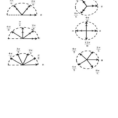
Fig. 1: Illustration of angle arrangements $\theta_{i}$’s for $N=6$, $7$ and $5$ respectively, using the $3$ rows of figures from top to bottom. The left figures represent the angle ($\theta_{i}$) for the columns of sensing matrices. Right figures are doubling those angles ($2\theta_{i}$) as in the objective function in (3.7).

4.3 $K=3$, $N\geq 7$ is an Odd Number

One might think that the uniform distributed design is optimal for $N\geq 7$. However, this is not true from the following theorem. Instead, the optimal design is to eliminate one angle from the optimal design for $(N+1)$.

Theorem 4.3

If $K=3$ and $N\geq 7$ is an odd number, then $\theta_{i}=\frac{2\pi(i-1)}{N+1}\mod\pi$, $1\leq i\leq N$, minimizes the maximum condition number among all sub-matrices with $K=3$ columns.

5 Simulation Results

We now present simulation results.

5.1 Worst Case Condition Number vs $N$

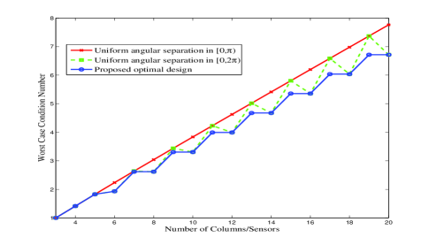
Fig. 2: Worst case condition number versus $N$

We compare the maximum condition number among all the possible $2\times 3$ submatrices in three different cases shown in Fig.2. The cases are, (i) when successive sensors are placed in a semicircle $\pi/N$ apart, namely $\theta_{i}=0,\frac{\pi}{N},...,\frac{\pi(N-1)}{N}$, (ii) they are placed $2\pi/N$ apart, namely $\theta_{i}=0,\frac{2\pi}{N},...,\frac{2\pi(N-1)}{N}$, and (iii) they are placed in a manner specified by our theorems. That the performance of (ii) matches (iii) for even $N$ conforms with earlier observations.

5.2 Worst Mean Square Signal Estimation Error vs $N$

Consider the setting of Section 1.1. We compare in Fig. 3 the mean square error (MSE) for worst-case submatrices yielded by (i) above with that yielded by the postulated optimum for sensors ranging in number from 3 to 15. The signal $x$ in (1.1) is $[9,9]^{T}$. The noise in each measurement is ${\cal N}\sim(0,1)$. For each value $N$, the estimation error $||\hat{x}-x||^{2}$ for worst-case submatrices was averaged over 2000 instances. Again the predicted optimal placement is superior.

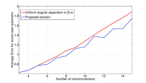
Fig. 3: Worst case estimation error versus the number of columns in the sensing matrix.

5.3 Monitoring Error vs SNR

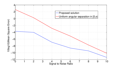
Fig. 4: Mean square error(dB) in the source location estimate when the worst performing subset of sensors are active versus the Signal to Noise Ratio(dB).

Fig. 4 compares the ML estimation of a source at the origin with $N=10$, from RSS under log-normal shadowing in the case where the sensors are placed as in (i) against optimal placement. The latter’s superiority is evident.

6 Conclusion and Future Work

We propose the problem designing optimal $M\times N$ ($M\leq N$) sensing matrices which minimize the maximum condition number of all the submatrices of $K$ columns. Such matrices minimize the worst-case estimation errors when only $K$ sensors out of $N$ sensors are available for sensing at a given time. When $M=2$ and $K=3$, for an arbitrary $N\geq 3$, we derive the optimal matrices which minimize the maximum condition number of all the submatrices of $K$ columns. It is interesting that minimizing the maximum coherence between columns does not always guarantee minimizing the maximum condition number.

References

- [1] I. Akyildiz and M. Vuran. Wireless Sensor Networks. Advanced Texts in Communications and Networking. John Wiley & Sons, 2010.
- [2] E. Candès. The restricted isometry property and its implications for compressed sensing. Comptes Rendus Mathematique, 2008.
- [3] M. Cardei and D.Z. Du. Improving wireless sensor network lifetime through power aware organization. Wireless Networks, 11(3):333–340, May 2005.
- [4] T. Cover and J. Thomas. Elements of Information Theory. 2nd Edition. Wiley, 2006.
- [5] S. Dasgupta, S. Ibeawuchi, and Z. Ding. Optimum sensor placement for source monitoring under log-normal shadowing, Proceedings of IFAC Symnposium on System Identification, Saint Malo, France, 2008.
- [6] S. Dasgupta, S. Ibeawuchi, and Z. Ding. Optimum sensor placement for source monitoring under log-normal shadowing in three dimensions. Proceedings of the 9th International Symposium on Communications and Information Technology, pages 376 –381, 2009.
- [7] A. Bishop, B. Fidan, B. Anderson, K. Dogancay and P. Pathirana, Optimality analysis of sensor-target localization geometries. In Automatica, pp. 479-492, 2010.
- [8] S. Martínez and F. Bullo, Optimal sensor placement and motion coordination for target tracking. Automatica, 42(4):661 – 668, 2006.
- [9] H. Godrich, A. Petropulu, and H.V. Poor. Sensor selection in distributed multiple-radar architectures for localization: A knapsack problem formulation. IEEE Transactions on Signal Processing, 60(1):247 –260, jan. 2012.
- [10] S. Ibeawuchi. Optimum sensor placement for source localization and monitoring from received signal strength, Ph.D dissertation, The University of Iowa, 2010.
- [11] E. Masazade, R. Niu, P. Varshney, and M. Keskinoz. Energy aware iterative source localization for wireless sensor networks. IEEE Transactions on Signal Processing, 58(9):4824 –4835, sept. 2010.
- [12] Y. Oshman. Optimal sensor selection strategy for discrete-time state estimators. IEEE Transactions on Aerospace and Electronic Systems, 30(2):307 –314, 1994.
- [13] T. Rappaport. Wireless communications: principles and practice. Prentice Hall communications engineering and emerging technologies series, 2002.
- [14] A. Savkin, R. Evans, and E. Skafidas. The problem of optimal robust sensor scheduling. In Proceedings of the 39th IEEE Conference on Decision and Control, volume 4, pages 3791 –3796, 2000.
- [15] L. Scharf and L. McWhorter. Geometry of the Cramer-Rao bound. Signal Processing, 31(3):301 – 311, 1993.
- [16] H. L. Van Trees, Detection, Estimation, and Modulation Theory: Detection, estimation, and linear modulation theory. Wiley, 2001.
- [17] B. Fidan, S, Dasgupta and B. Anderson, “Guaranteeing practical convergence in algorithms for sensor and source localization”, IEEE Transactions on Signal Processing, 56 (9), pp. 4458-4469, 2008.