Final state interaction effects in exclusive
electrodisintegration of the deuteron

S. G. Bondarenko
Joint Institute for Nuclear Research, Dubna, Russia
E-mail: bondarenko@jinr.ru
V. V. Burov
Joint Institute for Nuclear Research, Dubna, Russia
E-mail: burov@theor.jinr.ru
E. P. Rogochaya
Joint Institute for Nuclear Research, Dubna, Russia
E-mail: rogochaya@theor.jinr.ru

The exclusive electrodisintegration of the deuteron is considered within the Bethe-Salpeter approach with a separable interaction kernel. The relativistic kernel of nucleon-nucleon interaction is obtained considering the phase shifts in the elastic neutron-proton scattering and properties of the deuteron. The differential cross section is calculated within the impulse approximation under several kinematic conditions of the Bonn experiment. Final state interactions between the outgoing nucleons are taken into account. Partial-wave states of the neutron-proton pair with total angular momentum $J=0,1$ are considered.

1 Introduction

The exclusive electrodisintegration of the deuteron is a useful instrument which makes it possible to investigate the electromagnetic structure not only of the bound state - deuteron but also the scattering states of the neutron-proton ($np$) system. Many approaches have been elaborated to describe this reaction for the last 40 years [1, 2, 3, 4, 5]. The simplest of them considered the electrodisintegration within a nonrelativistic model of the nucleon-nucleon (NN) interaction and outgoing nucleons were supposed to be free [1] (the plane-wave approximation - PWA). Those approaches were in a good agreement with experimental data at low energies. However, further investigations have shown that the final state interaction (FSI) between outgoing nucleons, two-body currents and other effects should be taken into account to obtain a reasonable agreement with existing experimental data at higher energies. Most of these effects have been considered within nonrelativistic models [2, 3]. In relativistic models, FSI effects could be calculated within quasipotential approaches using the on-mass-shell nucleon-nucleon $T$ matrix [4, 5].

One of the fundamental approaches used to describe of the $np$ system is based on the Bethe-Salpeter (BS) equation [6]. The separable ansatz [7] for the NN interaction kernel was successfully applied to solve this equation. However, the approach was not applicable for the most of high-energy NN processes for a while since calculated expressions contained nonintegrable singularities. The problem was solved in [8, 9, 10] where kernels of special type were proposed. Using them FSI can be taken into account (in particular, considering the electrodisintegration) in a wide range of energy.

In the present paper, the electrodisintegration cross section is calculated under different kinematic conditions of Bonn experiments [11, 12]. The rank-six NN interaction potential MY6 [9] is used to describe scattered states ${}^{3}S_{1}$-${}^{3}D_{1}$ and the deuteron. The uncoupled partial-wave states with total angular momentum $J=0,1$ (${}^{1}S_{0}$, ${}^{1}P_{1}$, ${}^{3}P_{0}$, ${}^{3}P_{1}$) are described by multirank separable potentials [10].

The paper is organized as follows. In Sec.2, the exclusive three-differential cross section of the $d(e,e^{\prime}p)n$ reaction is calculated within the relativistic impulse approximation. The used BS formalism is presented in Sec.3. The details of calculations are considered in Sec.4. Then the obtained relativistic results are compared with experimental data of the Bonn experiments [11, 12] in Sec.5.

2 Cross section

When all particles are unpolarized the exclusive electrodisintegration of the deuteron $d(e,e^{\prime}p)n$ can be described by the differential cross section in the deuteron rest frame - laboratory system (LS), which has the following form:

$$\frac{d^{3}\sigma}{dE_{e}^{\prime}d\Omega_{e}^{\prime}d\Omega_{p}}=\frac{\sigma_{\textmd{Mott}}}{8M_{d}(2\pi)^{3}}{\frac{{\mbox{\boldmath$p$}}_{p}^{2}{\sqrt{s}}}{\sqrt{1+\eta}|{\mbox{\boldmath$p$}}_{p}|-E_{p}\sqrt{\eta}\cos\theta_{p}}}$$ (1)

$$\times\left[l^{0}_{00}W_{00}+l^{0}_{++}(W_{++}+W_{--})+2l^{0}_{+-}\cos 2\phi~{}{\rm Re}W_{+-}-2l^{0}_{+-}\sin 2\phi~{}{\rm Im}W_{+-}\right.$$

$$\hskip 14.22636pt\left.-2l^{0}_{0+}\cos\phi~{}{\rm Re}(W_{0+}-W_{0-})-2l^{0}_{0+}\sin\phi~{}{\rm Im}(W_{0+}+W_{0-})\right].$$

where $\sigma_{\rm Mott}=(\alpha\cos\frac{\theta}{2}/2E_{e}\sin^{2}\frac{\theta}{2})^{2}$ is the Mott cross section, $\alpha={e^{2}}/{(4\pi)}$ is the fine structure constant; $M_{d}$ is the mass of the deuteron; $q=p_{e}-p_{e}^{\prime}=(\omega,{\mbox{\boldmath$q$}})$ is the momentum transfer; $p_{e}=(E_{e},{\mbox{\boldmath$l$}})$ and $p_{e}^{\prime}=(E_{e}^{\prime},{\mbox{\boldmath$l$}}^{\prime})$ are initial and final electron momenta, respectively; $\Omega_{e}^{\prime}$ is the outgoing electron solid angle; $\theta$ is the electron scattering angle. The outgoing proton is described by momentum ${\mbox{\boldmath$p$}}_{p}$ ($E_{p}=\sqrt{{\mbox{\boldmath$p$}}_{p}^{2}+m^{2}}$, $m$ is the mass of the nucleon) and solid angle $\Omega_{p}=(\theta_{p},\phi)$ where $\theta_{p}$ is the zenithal angle between the ${\mbox{\boldmath$p$}}_{p}$ and $q$ momenta and $\phi$ is the azimuthal angle between the (ee^′) and (qp) planes. Factor $\eta={\mbox{\boldmath$q$}}^{2}/s$ can be calculated through the $np$ pair total momentum $P$ squared:

$$s=P^{2}=(p_{p}+p_{n})^{2}=M_{d}^{2}+2M_{d}\omega+q^{2},$$ (2)

defined by the sum of the proton $p_{p}$ and neutron $p_{n}$ momenta. The photon density matrix elements have the following form:

$$l_{00}^{0}=\frac{Q^{2}}{{\mbox{\boldmath$q$}}^{2}},\quad l_{0+}^{0}=\frac{Q}{|{\mbox{\boldmath$q$}}|\sqrt{2}}\sqrt{\frac{Q^{2}}{{\mbox{\boldmath$q$}}^{2}}+\tan^{2}\frac{\theta}{2}},l_{++}^{0}=\tan^{2}\frac{\theta}{2}+\frac{Q^{2}}{2{\mbox{\boldmath$q$}}^{2}},\quad l_{+-}^{0}=-\frac{Q^{2}}{2{\mbox{\boldmath$q$}}^{2}},$$ (3)

where $Q^{2}=-q^{2}$ is introduced for convenience. The hadron density matrix elements have the following form:

$$W_{\lambda\lambda^{\prime}}=W_{\mu\nu}\varepsilon_{\lambda}^{\mu}\varepsilon_{\lambda^{\prime}}^{\nu},$$ (4)

where $\lambda$, $\lambda^{\prime}$ are photon helicity components [13], can be calculated using the photon polarization vectors $\varepsilon$ and Cartesian components of hadron tensor

$$W_{\mu\nu}=\frac{1}{3}\sum_{s_{d}s_{n}s_{p}}\left|<np:SM_{S}|j_{\mu}|d:1M>\right|^{2},$$ (5)

where $S$ is the spin of the $np$ pair and $M_{S}$ is its projection; $s_{d}$, $s_{n}$ and $s_{p}$ are deuteron, neutron and proton momentum projections, respectively. The matrix element $<np:SM_{S}|j_{\mu}|d:1M>$ can be written using the Mandelstam technique [14] as follows:

$$<np:SM_{S}|j_{\mu}|d:1M>=i\sum_{n=1,2}\int\frac{d^{4}p^{\rm\mbox{\tiny CM}}}{(2\pi)^{4}}{\rm Sp}\left\{\Lambda({\cal L}^{-1})\bar{\psi}_{SM_{S}}(p^{\rm\mbox{\tiny CM}},{p^{*}}^{\rm\mbox{\tiny CM}};P^{\rm\mbox{\tiny CM}})\Lambda({\cal L})\right.\times$$ (6)

$$\hskip 85.35826pt\Gamma_{\mu}^{(n)}(q)S^{(n)}\left(\frac{K_{(0)}}{2}-(-1)^{n}p-\frac{q}{2}\right)\left.\Gamma^{M}\left(p+(-1)^{n}\frac{q}{2};K_{(0)}\right)\right\}$$

within the relativistic impulse approximation in LS. The sum over $n=1,2$ corresponds to the interaction of the virtual photon with proton and with neutron in the deuteron, respectively. The total $P^{\rm\mbox{\tiny CM}}$ and relative ${p^{*}}^{\rm\mbox{\tiny CM}}$ momenta of the outgoing nucleons and the integration momentum $p^{\rm\mbox{\tiny CM}}$ are considered in the final $np$ pair rest frame - center-of-mass system (CMS), $p$ denotes the relative $np$ pair momentum in LS. To perform the integration, momenta $p$, $q$ and deuteron total momentum $K_{(0)}=(M_{d},{\mbox{\boldmath$0$}})$ in LS are written in CMS using the Lorenz-boost transformation ${\cal L}$ along the $q$ direction. The $np$ pair wave function $\psi_{SM_{S}}$ is transformed from CMS to LS applying the corresponding boost operator $\Lambda$. A detailed description of $\psi_{SM_{S}}$, the $n$th nucleon interaction vertex $\Gamma_{\mu}^{(n)}$, the propagator of the $n$th nucleon $S^{(n)}$, and the deuteron vertex function $\Gamma^{M}$ can be found in our previous works [15, 16].

3 Separable kernel of NN interaction

The outgoing $np$ pair is described by the $T$ matrix which can be found solving the inhomogeneous Bethe-Salpeter equation [6]:

$$T(p^{\prime},p;P)=V(p^{\prime},p;P)+\frac{i}{4\pi^{3}}\int d^{4}k\,V(p^{\prime},k;P)\,S_{2}(k;P)\,T(k,p;P),$$ (7)

where $V$ is the NN interaction kernel, $S_{2}$ is the free two-particle Green function:

$$S_{2}^{-1}(k;P)=\bigl{(}\tfrac{1}{2}\>{\not{P}}+{\not{k}}-m\bigr{)}^{(1)}\bigl{(}\tfrac{1}{2}\>{\not{P}}-{\not{k}}-m\bigr{)}^{(2)},$$ (8)

and $p~{}(p^{\prime})$ is the relative momentum of initial (final) nucleons, $P$ is the total $np$ pair momentum.

To solve the BS equation (7) partial-wave decomposition [17] for the $T$ matrix:

$$T_{\alpha\beta,\gamma\delta}(p^{\prime},p;{P_{(0)}})=\sum_{JMab}t_{ab}(p_{0}^{\prime},|{\mbox{\boldmath$p^{\prime}$}}|;p_{0},|{\mbox{\boldmath$p$}}|;s)({\cal Y}_{aM}(-{{\mbox{\boldmath$p^{\prime}$}}})U_{C})_{\alpha\beta}\otimes(U_{C}{\cal Y}^{{\dagger}}_{bM}({{\mbox{\boldmath$p$}}}))_{\delta\gamma}$$ (9)

is used. Here $P_{(0)}=(\sqrt{s},{\mbox{\boldmath$0$}})$ is the $np$ pair total momentum in CMS, $U_{C}=i\gamma^{2}\gamma^{0}$ is the charge conjugation matrix. Indices $a,b$ correspond to the set ${}^{2S+1}L_{J}^{\rho}$ of spin $S$, orbital $L$ and total $J$ angular momenta, $\rho=+$ defines a positive-energy partial-wave state, $\rho=-$ corresponds to a negative-energy one. Greek letters $\{\alpha,\beta,\gamma,\delta\}$ in (9) are used to denote Dirac matrix indices. The spin-angle functions:

$${\cal Y}_{JM:LS{\rho}}({\mbox{\boldmath$p$}})U_{C}=i^{L}\sum_{m_{L}m_{S}m_{1}m_{2}\rho_{1}\rho_{2}}C_{\frac{1}{2}\rho_{1}\frac{1}{2}\rho_{2}}^{S_{\rho}{\rho}}C_{Lm_{L}Sm_{S}}^{JM}C_{\frac{1}{2}m_{1}\frac{1}{2}m_{2}}^{Sm_{S}}Y_{L{m_{L}}}(\hat{\mbox{\boldmath$p$}}){U^{\rho_{1}}_{m_{1}}}^{(1)}({\mbox{\boldmath$p$}}){{U^{\rho_{2}}_{m_{2}}}^{(2)}}^{T}(-{\mbox{\boldmath$p$}})$$

are constructed using free nucleon Dirac spinors $u,~{}v$. It should be mentioned that only positive-energy states with $\rho=+$ are considered in this paper. Performing similar decomposition for $V$, the BS equation for radial parts of the $T$ matrix and kernel $V$ is obtained:

$$t_{ab}(p_{0}^{\prime},|{\mbox{\boldmath$p^{\prime}$}}|;p_{0},|{\mbox{\boldmath$p$}}|;s)=v_{ab}(p_{0}^{\prime},|{\mbox{\boldmath$p^{\prime}$}}|;p_{0},|{\mbox{\boldmath$p$}}|;s)$$ (10)

$$+\frac{i}{4\pi^{3}}\sum_{cd}\int\limits_{-\infty}^{+\infty}\!dk_{0}\int\limits_{0}^{\infty}\!{\mbox{\boldmath$k$}}^{2}d|{\mbox{\boldmath$k$}}|\,v_{ac}(p_{0}^{\prime},|{\mbox{\boldmath$p^{\prime}$}}|;k_{0},|{\mbox{\boldmath$k$}}|;s)S_{cd}(k_{0},|{\mbox{\boldmath$k$}}|;s)\,t_{db}(k_{0},|{\mbox{\boldmath$k$}}|;p_{0},|{\mbox{\boldmath$p$}}|;s).$$

To solve the resulting equation (10), a separable ansatz [7] for the interaction kernel $v$ is used:

$$v_{ab}(p_{0}^{\prime},|{\mbox{\boldmath$p^{\prime}$}}|;p_{0},|{\mbox{\boldmath$p$}}|;s)=\sum_{i,j=1}^{N}\lambda_{ij}(s)g_{i}^{[a]}(p_{0}^{\prime},|{\mbox{\boldmath$p^{\prime}$}}|)g_{j}^{[b]}(p_{0},|{\mbox{\boldmath$p$}}|),$$ (11)

where $N$ is a rank of a separable kernel, $g_{i}$ are model functions, $\lambda_{ij}$ is a parameter matrix. Substituting $v$ (11) into BS equation (7), we obtain the $t$ matrix in a similar separable form:

$$t_{ab}(p_{0}^{\prime},|{\mbox{\boldmath$p^{\prime}$}}|;p_{0},|{\mbox{\boldmath$p$}}|;s)=\sum_{i,j=1}^{N}\tau_{ij}(s)g_{i}^{[a]}(p_{0}^{\prime},|{\mbox{\boldmath$p^{\prime}$}}|)g_{j}^{[b]}(p_{0},|{\mbox{\boldmath$p$}}|)$$ (12)

where:

$$\tau_{ij}(s)=1/(\lambda_{ij}^{-1}(s)+h_{ij}(s)),$$ (13)

and

$$h_{ij}(s)=-\frac{i}{4\pi^{3}}\sum_{a}\int dk_{0}\int{\mbox{\boldmath$k$}}^{2}d|{\mbox{\boldmath$k$}}|\frac{g_{i}^{[a]}(k_{0},|{\mbox{\boldmath$k$}}|)g_{j}^{[a]}(k_{0},|{\mbox{\boldmath$k$}}|)}{(\sqrt{s}/2-E_{\mbox{\scriptsize k}}+i\epsilon)^{2}-k_{0}^{2}}$$ (14)

are auxiliary functions, $E_{\mbox{\scriptsize k}}=\sqrt{{\mbox{\boldmath$k$}}^{2}+m^{2}}$. Thus, the problem of solving the initial integral BS equation (7) turns out to finding functions $g_{i}$ and parameters $\lambda_{ij}$ of separable representation (11). They can be obtained from a description of observables in $np$ elastic scattering [9, 10, 18, 19, 20].

4 Final state interaction

To calculate FSI we need to consider the interacting $np$ pair. The outgoing nucleons are described by the BS amplitude which can be written as a sum of two terms:

$$\psi_{SM_{S}}(p,p^{*};P)=\psi^{(0)}_{SM_{S}}(p,p^{*};P)+\frac{i}{4\pi^{3}}S_{2}(p;P)\int d^{4}k~{}V(p,k;P)\psi_{SM_{S}}(k,p^{*};P).$$ (15)

The first term

$$\psi_{SM_{S}}^{(0)}(p,p^{*};P)=(2\pi)^{4}\chi_{SM_{S}}(p;P)\delta(p-p^{*})$$ (16)

is related to the outgoing pair of free nucleons, $\chi_{SM_{S}}$ is a spinor function for two fermions. The second term in (15) corresponds to the final state interaction of the outgoing nucleons. If we use the following relation:

$$\int d^{4}k~{}V(p,k;P)\psi_{SM_{S}}(k,p^{*};P)=\int d^{4}k~{}T(p,k;P)\psi^{(0)}_{SM_{S}}(k,p^{*};P)$$

then it can be transformed into

$$\psi_{SM_{S}}^{(t)}(p,p^{*};P)=4\pi iS_{2}(p;P)T(p,p^{*};P)\chi_{SM_{S}}(p^{*};P),$$ (17)

here $(t)$ means that this part of the $np$ pair wave function is related to the $T$ matrix. Using the partial-wave decomposition (9) expression (17) can be written as follows:

$$\psi_{SM_{S}}^{(t)}(p,p^{*};P)=4\pi i\sum_{LmJMa}C_{LmSM_{S}}^{JM}Y_{Lm}^{*}(\hat{\mbox{\boldmath$p$}}^{*}){\cal Y}_{aM}({\mbox{\boldmath$p$}})\phi_{a,J:LS+}(p_{0},|{\mbox{\boldmath$p$}}|;s),$$ (18)

where $p^{*}=(0,{\mbox{\boldmath$p$}}^{*})$ with $|{\mbox{\boldmath$p$}}^{*}|=\sqrt{s/4-m^{2}}$ is the relative momentum of on-mass-shell nucleons in CMS, $\hat{\mbox{\boldmath$p$}}^{*}$ denotes the azimuthal angle $\theta_{\mbox{\scriptsize{p${}^{*}$}}}$ between the ${\mbox{\boldmath$p$}}^{*}$ and $q$ vectors and zenithal angle $\phi$. Since only positive-energy partial-wave states are considered here the radial part is:

$$\phi_{a,J:LS+}(p_{0},|{\mbox{\boldmath$p$}}|;s)=\frac{t_{a,J:LS+}(p_{0},|{\mbox{\boldmath$p$}}|;0,|{\mbox{\boldmath$p$}}^{*}|;s)}{(\sqrt{s}/2-E_{\mbox{\scriptsize p}}+i\epsilon)^{2}-p_{0}^{2}}.$$ (19)

According to definition (3) spin-angle functions ${\cal Y}$ can be written as a product of Dirac matrices $\gamma$ in the matrix representation [15] as follows:

$${\cal Y}_{aM}({\mbox{\boldmath$p$}})=\frac{1}{\sqrt{8\pi}}\frac{1}{4E_{\mbox{\scriptsize p}}(E_{\mbox{\scriptsize p}}+m)}(m+{\not{p}}_{1})(1+\gamma_{0}){\cal G}_{aM}(m-{\not{p}}_{2}),$$ (20)

matrices ${\cal G}_{aM}$ are shown in Table 1. Decomposition (18) is considered in detail in [22].

$a={\footnotesize\left\{{}^{2S+1}L_{J}^{\rho}\right\}^{{\phantom{1}}^{\phantom{1}}}}$	${\cal G}_{aM}$
$~{}{{}^{1}S_{0}^{+}}^{{\phantom{1}}^{\phantom{1}}}$	$-\gamma_{5}$
$~{}^{3}S_{1}^{+}$	${\not{\xi}}_{M}$
$~{}^{1}P_{1}^{+}$	$\frac{\sqrt{3}}{|{\mbox{\boldmath$p$}}|}(p_{1}\cdot\xi_{M})\gamma_{5}$
$~{}^{3}P_{0}^{+}$	$-\frac{1}{2|{\mbox{\boldmath$p$}}|}({\not{p}_{1}}-{\not{p}_{2}})$
$~{}^{3}P_{1}^{+}$	$-\sqrt{\frac{3}{2}}\frac{1}{|{\mbox{\boldmath$p$}}|}\left[(p_{1}\cdot\xi_{M})-\frac{1}{2}{\not{\xi}}_{M}({\not{p}_{1}}-{\not{p}_{2}})\right]\gamma_{5}$
$~{}^{3}D_{1}^{+}$	$\frac{1}{\sqrt{2}}\left[{\not{\xi}}_{M}+\frac{3}{2}\frac{1}{{\mbox{\boldmath$p$}}^{2}}(p_{1}\cdot\xi_{M})({\not{p}}_{1}-{\not{p}}_{2})\right]$

Table 1: Spin-angular parts ${\cal G}_{aM}$ (20) for the $np$ pair; $p_{1}=(E_{\mbox{\scriptsize p}},{\mbox{\boldmath$p$}})$, $p_{2}=(E_{\mbox{\scriptsize p}},-{\mbox{\boldmath$p$}})$ are on-mass-shell momenta, $E_{\mbox{\scriptsize p}}=\sqrt{{\mbox{\boldmath$p$}}^{2}+m^{2}}$; $\gamma$ matrices are defined as in [21].

Using definition (15) and substituting (16), (18) into (6), the final expression for hadron current
$<np:SM_{S}|j_{\mu}|d:1M>$ can be obtained. It consists of two parts. One of them:

$$<np:SM_{S}|j_{\mu}|d:1M>^{(0)}=i\sum_{n=1,2}\left\{\Lambda({\cal L}^{-1})\bar{\chi}_{SM_{S}}\left({p^{*}}^{\rm\mbox{\tiny CM}};P^{\rm\mbox{\tiny CM}}\right)\Lambda({\cal L})\right.\times$$ (21)

$$\Gamma_{\mu}^{(n)}(q)S^{(n)}\left(\frac{K_{(0)}}{2}-(-1)^{n}p^{*}-\frac{q}{2}\right)\left.\Gamma^{M}\left(p^{*}+(-1)^{n}\frac{q}{2};K_{(0)}\right)\right\}$$

corresponds to the electrodisintegration in PWA. Another one:

$$<np:SM_{S}|j_{\mu}|d:1M>^{(t)}=\hskip 293.06339pt$$ (22)

$$\frac{i}{4\pi^{3}}\sum_{n=1,2}\sum_{LmJM_{J}L^{\prime}lm^{\prime}}C_{LmSM_{S}}^{JM_{J}}Y_{Lm}(\hat{\mbox{\boldmath$p$}}^{*})\int\limits_{-\infty}^{\infty}dp_{0}^{\rm\mbox{\tiny CM}}\int\limits_{0}^{\infty}{({\mbox{\boldmath$p$}}^{\rm\mbox{\tiny CM}})}^{2}d|{\mbox{\boldmath$p$}}^{\rm\mbox{\tiny CM}}|\int\limits_{-1}^{1}d\cos\theta_{\mbox{\scriptsize p}}^{\rm\mbox{\tiny CM}}\int\limits_{0}^{2\pi}d\phi\times\hskip 71.13188pt$$

$${\rm Sp}\left\{\Lambda({\cal L}^{-1})\bar{\cal Y}_{JL^{\prime}SM_{J}}({\mbox{\boldmath$p$}}^{\rm\mbox{\tiny CM}})\Lambda({\cal L})\Gamma_{\mu}^{(n)}(q)\times\right.\left.S^{(n)}\left(\frac{K_{(0)}}{2}-(-1)^{n}p-\frac{q}{2}\right){\cal Y}_{1lSm^{\prime}}\left({\mbox{\boldmath$p$}}+(-1)^{n}\frac{{\mbox{\boldmath$q$}}}{2}\right)\right\}\times$$

$$\frac{t_{L^{\prime}L}^{*}(p^{\rm\mbox{\tiny CM}}_{0},|{\mbox{\boldmath$p$}}^{\rm\mbox{\tiny CM}}|;0,|{\mbox{\boldmath$p$}}^{*}|;s)}{(\sqrt{s}/2-E_{\mbox{\scriptsize p}}+i\epsilon)^{2}-p_{0}^{2}}g_{l}\left(p_{0}+(-1)^{n}\frac{\omega}{2},{\mbox{\boldmath$p$}}+(-1)^{n}\frac{{\mbox{\boldmath$q$}}}{2};K_{(0)}\right)$$

corresponds to the process when FSI is taken into account. Here $g_{l}$ denotes the radial part of the deuteron vertex function $\Gamma^{M}$. The part ${\rm Sp}\left\{\ldots\right\}$ has been calculated using the algebra manipulation package MAPLE. The three-dimensional integration over $p_{0}^{\rm\mbox{\tiny CM}}$, $|{\mbox{\boldmath$p$}}^{\rm\mbox{\tiny CM}}|$ and $\cos\theta_{\mbox{\scriptsize p}}^{\rm\mbox{\tiny CM}}$ has been performed numerically using the programming language FORTRAN.

		BI	BII	BIII	BIV	BV
$E_{e}$, GeV		1.464	1.569	1.2	1.2	1.2
$E_{e}^{\prime}$, GeV	min	1.175	1.118	0.895	0.895	0.895
	max			0.800	0.800	0.800
$\theta$, ∘		21	21	20.15	20.15	20.15
${\mbox{\boldmath$p$}}_{n}$, GeV/$c$	min	0.314	0.500	0.126	0.197	0.197
	max	0.660	0.773	0.564	0.423	0.488
$\theta_{n}$, ∘	min	60.53	74.60	142.32	155.72	165.36
	max	62.49	63.52	93.96	136.09	112.86
$\theta_{qe}$, ∘	min	61.94	45.57	59.56	51.52	51.25
	max	37.39	29.49	25.57	25.57	25.57
${\mbox{\boldmath$p$}}_{p}$, GeV/$c$	min	0.466	0.681	0.525	0.620	0.622
	max	0.664	0.791	0.834	0.929	0.889
$\theta_{p}$, ∘	min	35.82	45.12	8.42	7.52	4.47
	max	61.68	60.90	42.40	18.41	30.40
$\theta_{pe}$, ∘	min	97.77	90.68	68.00	44.00	56.00
	max	99.08	90.39
$\sqrt{s}$, GeV	min	1.9675	2.1375	1.98	2.04	2.04
	max	2.2125	2.3325	2.28	2.28	2.28
$\sqrt{s}-2m$, GeV	min	0.090	0.260	0.101	0.161	0.161
	max	0.335	0.455	0.401	0.401	0.401
$Q^{2}$, (GeV/$c$)2	min	0.257	0.255	0.154	0.145	0.145
	max	0.206	0.209	0.106	0.106	0.106
$\omega$, GeV	min	0.162	0.348	0.148	0.210	0.210
	max	0.422	0.568	0.476	0.476	0.476
$|{\mbox{\boldmath$q$}}|$, GeV/$c$	min	0.532	0.613	0.420	0.435	0.435
	max	0.620	0.729	0.577	0.577	0.577

Table 2: Kinematic conditions considered in the paper. Here all quantities are given in LS. In addition to those which are defined in the text, they are: angle $\theta_{qe}$ between the beam and the virtual photon; neutron momentum ${\mbox{\boldmath$p$}}_{n}$ and angle $\theta_{n}$ between the neutron and the virtual photon (${\mbox{\boldmath$p$}}_{p},\theta_{p}$ – the same for the proton); $\theta_{pe}$ ($\theta_{qe}$) – the angle between the beam and the proton (virtual photon).

5 Results and discussion

The calculations of the deuteron electrodisintegration within PWA were considered in [9, 16]. As it was shown in [3, 23], a contribution of FSI effects increases with increasing nucleon energies or/and momentum transfer. The reaction near the threshold was considered in [23] (Sacley experiments, see [24, 25]).

In the paper the differential cross section (1) has been calculated under five kinematic conditions of the Bonn experiments [11, 12] (described in Table 2) and is shown in Figs.2-5. The calculations have been performed within the relativistic impulse approximation for two different cases: when the outgoing nucleons are supposed to be free (PWA) and when the final state interaction between the nucleons is taken into account (FSI). The partial-wave states of the $np$ pair with total angular momentum $J=0,1$ have been considered. The used relativistic model consists of two parts: the separable potential MY6 [9] for the bound (deuteron) and scattered ${}^{3}S_{1}$-${}^{3}D_{1}$ states and separable potentials of various ranks [10] - for all other partial-wave states (${}^{1}S_{0}$, ${}^{1}P_{1}$, ${}^{3}P_{0}$, ${}^{3}P_{1}$).

In Figs.2-5, relativistic PWA (solid red line) and FSI (dashed blue line) calculations are shown as a function of $\sqrt{s}$.

As it is seen from Figs.2-5, the effect of FSI increases the cross section for kinematic conditions [11, 12].

In Fig.2, the calculation with FSI describes the experimental data on $\sqrt{s}$ from 2.15 GeV to 2.3 GeV and differs from experimental data starting from 2.3 GeV. Calculations of the cross section shown in Figs.2-2 require additional investigations at high $s$ (for instance, the influence of non-nucleon degrees of freedom).

In Figs.4-5, PWA and FSI calculations under the kinematic conditions [12] are shown. The effect of FSI is small at the threshold but it becomes bigger with increasing $\sqrt{s}$.

The inelasticity effects are nonzero for kinematic conditions of Bonn experiments [11, 12]. However, they will be discussed in a separate paper.

aaa

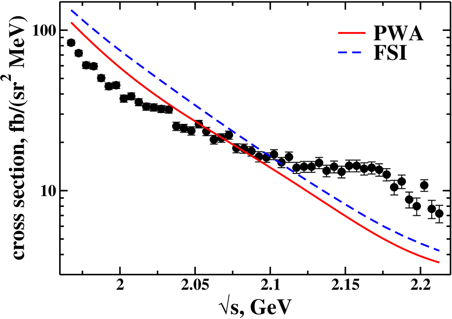
Figure 1: Cross section (1) depending on $\sqrt{s}$ calculated under kinematic conditions set I of the Bonn experiment [11].

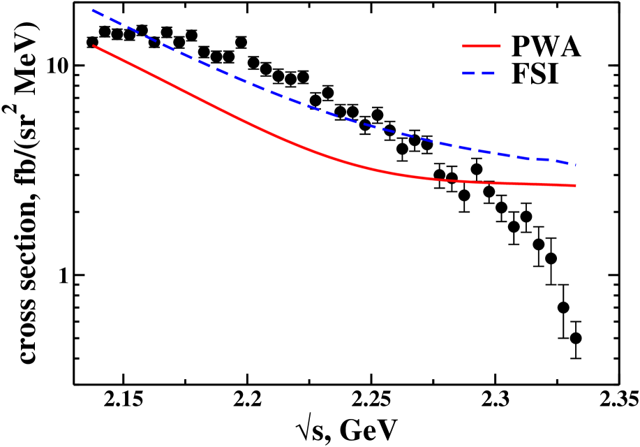
Figure 2: The same as in Fig.2 but under kinematic conditions set II of the Bonn experiment [11].

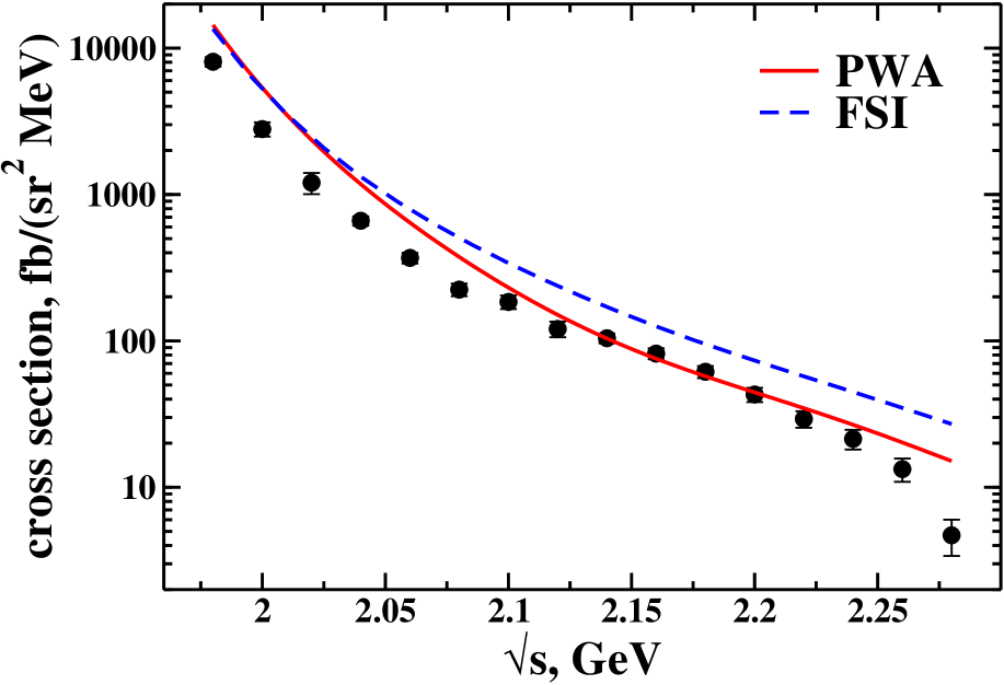
Figure 3: Cross section (1) depending $\sqrt{s}$ calculated under kinematic conditions set III of the Bonn experiment [12].

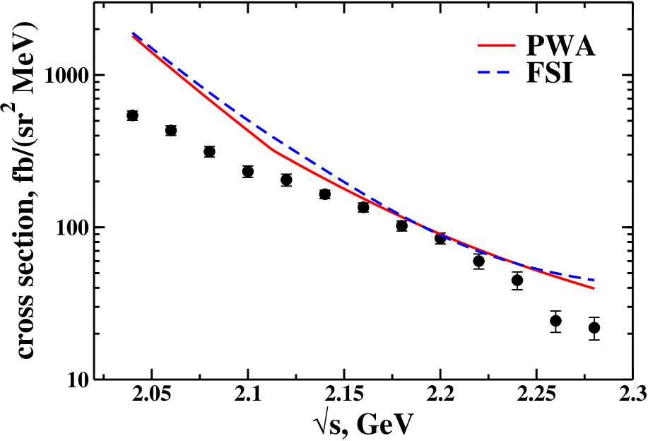
Figure 4: The same as in Fig.2 but under kinematic conditions set IV of the Bonn experiment [12].

aaa

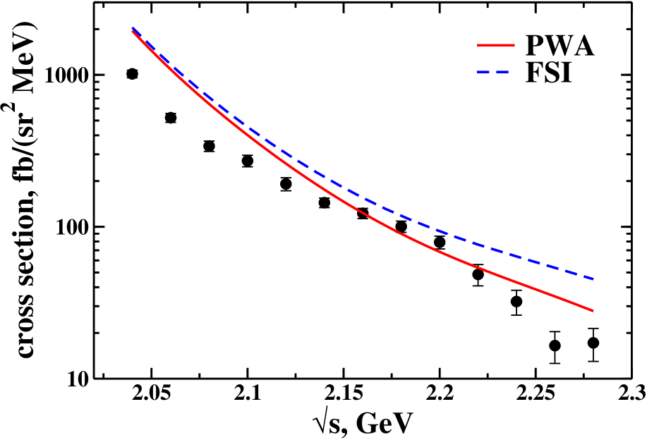
Figure 5: Cross section (1) depending on $\sqrt{s}$ calculated under kinematic conditions set V of the Bonn experiment [12].

References

• [1] T. De Forest, Nucl. Phys. A392, 232 (1983).
• [2] H. Arenhovel, Nucl. Phys. A384, 287 (1982).
• [3] A.Yu. Korchin, Yu.P. Melnik, and A.V. Shebeko, Sov. J. Nucl. Phys. 48, 243 (1988).
• [4] G.I. Gakh, A.P. Rekalo, and E. Tomasi-Gustafsson, Annals Phys. 319, 150 (2005).
• [5] S. Jeschonnek and J.W. Van Orden, Phys. Rev. C78, 014007 (2008).
• [6] E.E. Salpeter and H.A. Bethe, Phys. Rev. 84, 1232 (1951).
• [7] Y. Yamaguchi, Phys. Rev. 95, 1628 (1954);
Y. Yamaguchi and Y. Yamaguchi, Phys. Rev. 95, 1635 (1954).
• [8] S.G. Bondarenko, V.V. Burov, W-Y. Pauchy Hwang, and E.P. Rogochaya, JETP Lett. 87, 653 (2008).
• [9] S.G. Bondarenko, V.V. Burov, W.-Y.Pauchy Hwang, and E.P. Rogochaya, Nucl. Phys. A848, 75 (2010).
• [10] S.G. Bondarenko, V.V. Burov, W.-Y. Pauchy Hwang, and E.P. Rogochaya, Nucl. Phys. A832, 233 (2010).
• [11] H. Breuker et al., Nucl. Phys. A455, 641 (1986).
• [12] B. Boden et al., Nucl. Phys. A549, 471 (1992).
• [13] V. Dmitrasinovic and F. Gross, Phys. Rev. C40, 2479 (1989).
• [14] S. Mandelstam, Proc. Roy. Soc. Lond. A233, 248 (1955).
• [15] S.G. Bondarenko, V.V. Burov, A.V. Molochkov, G.I. Smirnov, and H. Toki, Prog. Part. Nucl. Phys. 48, 449 (2002).
• [16] S.G. Bondarenko, V.V. Burov, E.P. Rogochaya, and A.A. Goy, Phys. Part. Nucl. Lett. 2, 323 (2005);
S.G. Bondarenko, V.V. Burov, E.P. Rogochaya, and A.A. Goy, Phys. Atom. Nucl. 70, 2054 (2007).
• [17] J.J. Kubis, Phys. Rev. D6, 547 (1972).
• [18] G. Rupp and J.A. Tjon, Phys. Rev. C41, 472 (1990).
• [19] L. Mathelitsch, W. Plessas, and W. Schweiger, Phys. Rev. C26, 65 (1982).
• [20] S.G. Bondarenko, V.V. Burov, and E.P. Rogochaya, Phys.Lett. B705, 264-268 (2011); Nucl.Phys.Proc.Suppl. 219-220, 126-129 (2011).
• [21] J.D. Bjorken and S.D. Drell, Relativistic Quantum Mechanics and Relativistic Quantum Fields. McGraw-Hill, New York (1964).
• [22] S.G. Bondarenko, V.V. Burov, K.Yu. Kazakov, and D.V. Shulga, Phys. Part. Nucl. Lett. 1, 178 (2004).
• [23] S.G. Bondarenko, V.V. Burov, and E.P. Rogochaya, JETP Lett. 94, 3 (2012).
• [24] M. Bernheim et al., Nucl. Phys. A365, 349 (1981).
• [25] S. Turck-Chieze et al., Phys. Lett. B142, 145 (1984).