A convergent finite element approximation for the quasi-static Maxwell–Landau–Lifshitz–Gilbert equations thanks: Supported by the Australian Research Council under grant number DP120101886

Kim-Ngan Le School of Mathematics and Statistics, The University of New South Wales, Sydney 2052, Australia. Email: n.le-kim@student.unsw.edu.au, thanh.tran@unsw.edu.au    T. Tran
Abstract

We propose a θ𝜃\theta-linear scheme for the numerical solution of the quasi-static Maxwell–Landau–Lifshitz–Gilbert (MLLG) equations. Despite the strong nonlinearity of the Landau–Lifshitz–Gilbert equation, the proposed method results in a linear system at each time step. We prove that as the time and space steps tend to zero (with no further conditions when θ(12,1]𝜃121\theta\in(\frac{1}{2},1]), the finite element solutions converge weakly to a weak solution of the MLLG equations. Numerical results are presented to show the applicability of the method.

Key words: Maxwell–Landau–Lifshitz–Gilbert, finite element, ferromagnetism

AMS suject classifications: 65M12, 35K55

1 Introduction

The Maxwell–Landau–Lifshitz–Gilbert (MLLG) equations describe the electromagnetic behavior of a ferromagnetic material. In this paper, for simplicity, we suppose that there is a bounded cavity D~3~𝐷superscript3\widetilde{D}\subset{\mathbb{R}}^{3} (with perfectly conducting outer surface D~~𝐷\partial\widetilde{D}) into which a ferromagnet D𝐷D is embedded. We assume further that D~\D¯\~𝐷¯𝐷\widetilde{D}\backslash\bar{D} is a vacuum. We will consider the quasi-static case of the MLLG system. Letting DT:=(0,T)×Dassignsubscript𝐷𝑇0𝑇𝐷D_{T}:=(0,T)\times D and D~T:=(0,T)×D~assignsubscript~𝐷𝑇0𝑇~𝐷\widetilde{D}_{T}:=(0,T)\times\widetilde{D}, the magnetization field 𝒎:DT𝕊2:𝒎subscript𝐷𝑇superscript𝕊2\boldsymbol{m}:D_{T}\rightarrow\mathbb{S}^{2}, where 𝕊2superscript𝕊2\mathbb{S}^{2} is the unit sphere in 3superscript3{\mathbb{R}}^{3}, and the magnetic field 𝑯:D~T3:𝑯subscript~𝐷𝑇superscript3\boldsymbol{H}:\widetilde{D}_{T}\rightarrow\mathbb{R}^{3} satisfy

𝒎t=λ1𝒎×𝑯effλ2𝒎×(𝒎×𝑯eff) in DT,subscript𝒎𝑡subscript𝜆1𝒎subscript𝑯effsubscript𝜆2𝒎𝒎subscript𝑯eff in subscript𝐷𝑇\displaystyle\boldsymbol{m}_{t}=\lambda_{1}\boldsymbol{m}\times\boldsymbol{H}_{\text{eff}}-\lambda_{2}\boldsymbol{m}\times(\boldsymbol{m}\times\boldsymbol{H}_{\text{eff}})\quad\text{ in }D_{T}, (1.1)
μ0𝑯t+σ×(×𝑯)=μ0𝒎~t in D~T,subscript𝜇0subscript𝑯𝑡𝜎𝑯subscript𝜇0subscript~𝒎𝑡 in subscript~𝐷𝑇\displaystyle\mu_{0}\boldsymbol{H}_{t}+\sigma\nabla\times(\nabla\times\boldsymbol{H})=-\mu_{0}\widetilde{\boldsymbol{m}}_{t}\quad\text{ in }\widetilde{D}_{T}, (1.2)

in which λ10subscript𝜆10\lambda_{1}\not=0, λ2>0subscript𝜆20\lambda_{2}>0, σ0𝜎0\sigma\geq 0, and μ0>0subscript𝜇00\mu_{0}>0 are constants. Here 𝒎~:D~T3:~𝒎subscript~𝐷𝑇superscript3\widetilde{\boldsymbol{m}}:\widetilde{D}_{T}\rightarrow{\mathbb{R}}^{3} is the zero extension of 𝒎𝒎\boldsymbol{m} onto D~Tsubscript~𝐷𝑇\widetilde{D}_{T}, i.e.,

𝒎~(t,𝒙)={𝒎(t,𝒙),(t,𝒙)DT0,(t,𝒙)D~T\DT.~𝒎𝑡𝒙cases𝒎𝑡𝒙𝑡𝒙subscript𝐷𝑇0𝑡𝒙\subscript~𝐷𝑇subscript𝐷𝑇\widetilde{\boldsymbol{m}}(t,\boldsymbol{x})=\begin{cases}\boldsymbol{m}(t,\boldsymbol{x}),&\quad(t,\boldsymbol{x})\in D_{T}\\ \hfill 0,&\quad(t,\boldsymbol{x})\in\widetilde{D}_{T}\backslash D_{T}.\end{cases}

For simplicity the effective field 𝑯effsubscript𝑯eff\boldsymbol{H}_{\text{eff}} is taken to be 𝑯eff=Δ𝒎+𝑯subscript𝑯effΔ𝒎𝑯\boldsymbol{H}_{\text{eff}}=\Delta\boldsymbol{m}+\boldsymbol{H}.

The system (1.1)–(1.2) is supplemented with initial conditions

𝒎(0,.)=𝒎0 in Dand𝑯(0,.)=𝑯0 in D~,\boldsymbol{m}(0,.)=\boldsymbol{m}_{0}\text{ in }D\quad\text{and}\quad\boldsymbol{H}(0,.)=\boldsymbol{H}_{0}\text{ in }\widetilde{D}, (1.3)

and boundary conditions

n𝒎=0 on (0,T)×Dand(×𝑯)×n=0 on (0,T)×D~.formulae-sequencesubscript𝑛𝒎0 on 0𝑇𝐷and𝑯𝑛0 on 0𝑇~𝐷\partial_{n}\boldsymbol{m}=0\text{ on }(0,T)\times\partial D\quad\text{and}\quad(\nabla\times\boldsymbol{H})\times n=0\text{ on }(0,T)\times\partial\widetilde{D}. (1.4)

The equation (1.1) is the first dynamical model for the precessional motion of a magnetization, suggested by Landau and Lifshitz [12]. The existence and uniqueness of a local strong solution of (1.1)–(1.4) is shown by Cimrák [8]. He also proposes [7] a finite element method to approximate this local solution and provides error estimation.

Gilbert introduces a different approach for description of damped precession in [9]:

λ1𝒎t+λ2𝒎×𝒎t=μ𝒎×𝑯eff,subscript𝜆1subscript𝒎𝑡subscript𝜆2𝒎subscript𝒎𝑡𝜇𝒎subscript𝑯eff\displaystyle\lambda_{1}\boldsymbol{m}_{t}+\lambda_{2}\boldsymbol{m}\times\boldsymbol{m}_{t}=\mu\boldsymbol{m}\times\boldsymbol{H}_{\text{eff}}, (1.5)

in which μ=λ12+λ22𝜇superscriptsubscript𝜆12superscriptsubscript𝜆22\mu=\lambda_{1}^{2}+\lambda_{2}^{2}. A proof of the equivalence between (1.5) and (1.1) can be found in  [13]. It is easier to numerically solve (1.5) than (1.1) because the latter has a double cross term, namely 𝒎×(𝒎×𝑯eff)𝒎𝒎subscript𝑯eff\boldsymbol{m}\times(\boldsymbol{m}\times\boldsymbol{H}_{\text{eff}}).

Instead of solving (1.1)–(1.4), Baňas, Bartels and Prohl [2] propose an implicit nonlinear scheme to solve problem (1.2)–(1.5), and prove that the finite element solution converges to a weak global solution of the problem. Their method requires a condition on the time step k𝑘k and space step hh (namely k=O(h2)𝑘𝑂superscript2k=O(h^{2})) for the convergence of the nonlinear system of equations resulting from the discretization.

Following the idea developed by Alouges and Jaison [1] for the Landau–Lifshitz–Gilbert (LLG) equation (1.5), we propose a θ𝜃\theta-linear finite element scheme to find a weak global solution to (1.2)–(1.5). We prove that the numerical solutions converge to a weak solution of the problem with no condition imposed on time step and space step as θ(12,1]𝜃121\theta\in(\frac{1}{2},1]. It is required that k=o(h2)𝑘𝑜superscript2k=o(h^{2}) when θ[0,12)𝜃012\theta\in[0,\frac{1}{2}), and k=o(h)𝑘𝑜k=o(h) when θ=12𝜃12\theta=\frac{1}{2}. The implementation aspect of the algorithm is reported in [13] where no convergence analysis is carried out.

The paper is organized as follows. Weak solutions of the MLLG equations are defined in Section 2. We also introduce in this section the θ𝜃\theta-linear finite element scheme. Some technical lemmas are presented in Section 3. In Section 4, we prove that the finite element solutions converge to a weak solution of the MLLG equations. Numerical experiments are presented in the last section.

2 Weak solutions and finite element schemes

Before presenting the definition of a weak solution to the MLLG equations, it is necessary to introduce some function spaces and to assume some conditions on the initial functions 𝒎0subscript𝒎0\boldsymbol{m}_{0} and 𝑯0subscript𝑯0\boldsymbol{H}_{0}.

The function spaces 1(D,3)superscript1𝐷superscript3\mathbb{H}^{1}(D,{\mathbb{R}}^{3}) and (curl;D~)curl~𝐷\mathbb{H}(\operatorname{{curl\/}};\widetilde{D}) are defined as follows:

1(D,3)superscript1𝐷superscript3\displaystyle\mathbb{H}^{1}(D,{\mathbb{R}}^{3}) ={𝒖𝕃2(D,3):𝒖xi𝕃2(D,3)for i=1,2,3.},\displaystyle=\left\{\boldsymbol{u}\in\mathbb{L}^{2}(D,{\mathbb{R}}^{3}):\frac{\partial\boldsymbol{u}}{\partial x_{i}}\in\mathbb{L}^{2}(D,{\mathbb{R}}^{3})\quad\text{for }i=1,2,3.\right\},
(curl;D~)curl~𝐷\displaystyle\mathbb{H}(\operatorname{{curl\/}};\widetilde{D}) ={𝒖𝕃2(D~,3):×𝒖𝕃2(D~,3)}.absentconditional-set𝒖superscript𝕃2~𝐷superscript3𝒖superscript𝕃2~𝐷superscript3\displaystyle=\left\{\boldsymbol{u}\in\mathbb{L}^{2}(\widetilde{D},{\mathbb{R}}^{3}):\nabla\times\boldsymbol{u}\in\mathbb{L}^{2}(\widetilde{D},{\mathbb{R}}^{3})\right\}.

Here, for a domain Ω3Ωsuperscript3\Omega\subset{\mathbb{R}}^{3}, 𝕃2(Ω,3)superscript𝕃2Ωsuperscript3\mathbb{L}^{2}(\Omega,{\mathbb{R}}^{3}) is the usual space of Lebesgue squared integrable functions defined on ΩΩ\Omega and taking values in 3superscript3{\mathbb{R}}^{3}. Throughout this paper, we denote

,Ω:=,𝕃2(Ω,3)andΩ:=𝕃2(Ω,3).\displaystyle\left\langle{\cdot},{\cdot}\right\rangle_{\Omega}:=\left\langle{\cdot},{\cdot}\right\rangle_{\mathbb{L}^{2}(\Omega,{\mathbb{R}}^{3})}\quad\text{and}\quad\|\cdot\|_{\Omega}:=\|\cdot\|_{\mathbb{L}^{2}(\Omega,{\mathbb{R}}^{3})}.

In order to define a weak solution of MLLG equations, we assume that the given functions 𝒎0subscript𝒎0\boldsymbol{m}_{0} and 𝑯0subscript𝑯0\boldsymbol{H}_{0} satisfy

𝒎01(D,3),|𝒎0|=1 a.e. in Dand𝑯0(curl;D~).formulae-sequencesubscript𝒎0superscript1𝐷superscript3formulae-sequencesubscript𝒎01 a.e. in 𝐷andsubscript𝑯0curl~𝐷\boldsymbol{m}_{0}\in\mathbb{H}^{1}(D,{\mathbb{R}}^{3}),\quad|\boldsymbol{m}_{0}|=1\text{\ a.e. in }D\quad\text{and}\quad\boldsymbol{H}_{0}\in\mathbb{H}(\operatorname{{curl\/}};\widetilde{D}). (2.1)

For physical reasons (see [10]), these initial fields must satisfy

div(𝑯0+χD𝒎0)=0 in D~and(𝑯0+χD𝒎0)𝒏=0 on D~.formulae-sequencedivsubscript𝑯0subscript𝜒𝐷subscript𝒎00 in ~𝐷andsubscript𝑯0subscript𝜒𝐷subscript𝒎0𝒏0 on ~𝐷\operatorname{{div\/}}(\boldsymbol{H}_{0}+\chi_{D}\boldsymbol{m}_{0})=0\text{ in }\widetilde{D}\quad\text{and}\quad(\boldsymbol{H}_{0}+\chi_{D}\boldsymbol{m}_{0})\cdot\boldsymbol{n}=0\text{ on }\partial\widetilde{D}. (2.2)

Since equations (1.1) and (1.5) are equivalent (a proof of which can be found in [13]), instead of solving (1.1)–(1.4) we solve (1.2)–(1.5). A weak solution of the problem is defined in the following definition.

Definition 2.1.

Let the initial data (𝐦0,𝐇0)subscript𝐦0subscript𝐇0(\boldsymbol{m}_{0},\boldsymbol{H}_{0}) satisfy (2.1) and (2.2). Then (𝐦,𝐇)𝐦𝐇(\boldsymbol{m},\boldsymbol{H}) is call a weak solution to (1.2)–(1.5) if, for all T>0𝑇0T>0, there hold

  1. 1.

    𝒎1(DT,3)) and |𝒎|=1 a.e. in DT;\boldsymbol{m}\in\mathbb{H}^{1}(D_{T},\mathbb{R}^{3}))\text{ and }|\boldsymbol{m}|=1\text{ a.e. in }D_{T};

  2. 2.

    𝑯,𝑯t,×𝑯𝕃2(D~T,3)𝑯subscript𝑯𝑡𝑯superscript𝕃2subscript~𝐷𝑇superscript3\boldsymbol{H},\boldsymbol{H}_{t},\nabla\times\boldsymbol{H}\in\mathbb{L}^{2}(\widetilde{D}_{T},\mathbb{R}^{3});

  3. 3.

    for all ϕ(DT)bold-italic-ϕsuperscriptsubscript𝐷𝑇\boldsymbol{\phi}\in\mathbb{C}^{\infty}(D_{T}) and 𝜻(D~T)𝜻superscriptsubscript~𝐷𝑇\boldsymbol{\zeta}\in\mathbb{C}^{\infty}(\widetilde{D}_{T}),

    λ1𝒎t,ϕDT+λ2𝒎×𝒎t,ϕDT=μ𝒎,(𝒎×ϕ)DT+μ𝒎×𝑯,ϕDTsubscript𝜆1subscriptsubscript𝒎𝑡bold-italic-ϕsubscript𝐷𝑇subscript𝜆2subscript𝒎subscript𝒎𝑡bold-italic-ϕsubscript𝐷𝑇𝜇subscript𝒎𝒎bold-italic-ϕsubscript𝐷𝑇𝜇subscript𝒎𝑯bold-italic-ϕsubscript𝐷𝑇\displaystyle\lambda_{1}\left\langle{\boldsymbol{m}_{t}},{\boldsymbol{\phi}}\right\rangle_{D_{T}}+\lambda_{2}\left\langle{\boldsymbol{m}\times\boldsymbol{m}_{t}},{\boldsymbol{\phi}}\right\rangle_{D_{T}}=\mu\left\langle{\nabla\boldsymbol{m}},{\nabla(\boldsymbol{m}\times\boldsymbol{\phi})}\right\rangle_{D_{T}}+\mu\left\langle{\boldsymbol{m}\times\boldsymbol{H}},{\boldsymbol{\phi}}\right\rangle_{D_{T}} (2.3)

    and

    μ0𝑯t,𝜻D~T+σ×𝑯,×𝜻D~T=μ0𝒎~t,𝜻D~T,subscript𝜇0subscriptsubscript𝑯𝑡𝜻subscript~𝐷𝑇𝜎subscript𝑯𝜻subscript~𝐷𝑇subscript𝜇0subscriptsubscript~𝒎𝑡𝜻subscript~𝐷𝑇\mu_{0}\left\langle{\boldsymbol{H}_{t}},{\boldsymbol{\zeta}}\right\rangle_{\widetilde{D}_{T}}+\sigma\left\langle{\nabla\times\boldsymbol{H}},{\nabla\times\boldsymbol{\zeta}}\right\rangle_{\widetilde{D}_{T}}=-\mu_{0}\left\langle{\widetilde{\boldsymbol{m}}_{t}},{\boldsymbol{\zeta}}\right\rangle_{\widetilde{D}_{T}}, (2.4)

    where μ=λ12+λ22𝜇superscriptsubscript𝜆12superscriptsubscript𝜆22\mu=\lambda_{1}^{2}+\lambda_{2}^{2};

  4. 4.

    in the sense of traces there holds

    𝒎(0,)=𝒎0,𝒎0subscript𝒎0\boldsymbol{m}(0,\cdot)=\boldsymbol{m}_{0}, (2.5)
  5. 5.

    for almost all T(0,T)superscript𝑇0𝑇T^{\prime}\in(0,T),

    (T)+λ2μ1𝒎tDT2+λ2μ1𝑯tD~T2+2μ01σ×𝑯D~T2(0),superscript𝑇subscript𝜆2superscript𝜇1subscriptsuperscriptnormsubscript𝒎𝑡2subscript𝐷superscript𝑇subscript𝜆2superscript𝜇1subscriptsuperscriptnormsubscript𝑯𝑡2subscript~𝐷superscript𝑇2superscriptsubscript𝜇01𝜎subscriptsuperscriptnorm𝑯2subscript~𝐷superscript𝑇0\displaystyle{\cal E}(T^{\prime})+\lambda_{2}\mu^{-1}\|\boldsymbol{m}_{t}\|^{2}_{D_{T^{\prime}}}+\lambda_{2}\mu^{-1}\|\boldsymbol{H}_{t}\|^{2}_{\widetilde{D}_{T^{\prime}}}+2\mu_{0}^{-1}\sigma\|\nabla\times\boldsymbol{H}\|^{2}_{\widetilde{D}_{T^{\prime}}}\leq{\cal E}(0), (2.6)

    where

    (T)=𝒎(T)D2+𝑯(T)D~2+λ2μ1μ01σ×𝑯(T)D~2.superscript𝑇subscriptsuperscriptnorm𝒎superscript𝑇2𝐷subscriptsuperscriptnorm𝑯superscript𝑇2~𝐷subscript𝜆2superscript𝜇1superscriptsubscript𝜇01𝜎subscriptsuperscriptnorm𝑯superscript𝑇2~𝐷{\cal E}(T^{\prime})=\|\nabla\boldsymbol{m}(T^{\prime})\|^{2}_{D}+\|\boldsymbol{H}(T^{\prime})\|^{2}_{\widetilde{D}}+\lambda_{2}\mu^{-1}\mu_{0}^{-1}\sigma\|\nabla\times\boldsymbol{H}(T^{\prime})\|^{2}_{\widetilde{D}}.

We next introduce the θ𝜃\theta-linear finite element scheme which approximates a weak solution (𝒎,𝑯)𝒎𝑯(\boldsymbol{m},\boldsymbol{H}) defined in Definition 2.1.

Let 𝕋hsubscript𝕋\mathbb{T}_{h} be a regular tetrahedrization of the domain D~~𝐷\widetilde{D} into tetrahedra of maximal mesh-size hh, and let 𝕋h|Devaluated-atsubscript𝕋𝐷\mathbb{T}_{h}|_{D} be its restriction to DD~𝐷~𝐷D\subset\widetilde{D}. We denote by 𝒩h:={𝒙1,,𝒙N}assignsubscript𝒩subscript𝒙1subscript𝒙𝑁{\cal N}_{h}:=\{\boldsymbol{x}_{1},\ldots,\boldsymbol{x}_{N}\} the set of vertices and by h:={e1,,eM}assignsubscriptsubscript𝑒1subscript𝑒𝑀{\cal M}_{h}:=\{e_{1},\ldots,e_{M}\} the set of edges.

To discretize the LLG equation (2.3), we introduce the finite element space 𝕍h1(D,3)subscript𝕍superscript1𝐷superscript3\mathbb{V}_{h}\subset\mathbb{H}^{1}(D,{\mathbb{R}}^{3}) which is the space of all continuous piecewise linear functions on 𝕋h|Devaluated-atsubscript𝕋𝐷\mathbb{T}_{h}|_{D}. A basis for 𝕍hsubscript𝕍\mathbb{V}_{h} can be chosen to be (ϕn)1nNsubscriptsubscriptitalic-ϕ𝑛1𝑛𝑁(\phi_{n})_{1\leq n\leq N}, where ϕn(𝒙m)=δn,m.subscriptitalic-ϕ𝑛subscript𝒙𝑚subscript𝛿𝑛𝑚\phi_{n}(\boldsymbol{x}_{m})=\delta_{n,m}. Here δn,msubscript𝛿𝑛𝑚\delta_{n,m} stands for the Kronecker symbol. The interpolation operator from 0(D,3)superscript0𝐷superscript3{\mathbb{C}}^{0}(D,{\mathbb{R}}^{3}) onto 𝕍hsubscript𝕍\mathbb{V}_{h} is denoted by I𝕍hsubscript𝐼subscript𝕍I_{\mathbb{V}_{h}},

I𝕍h(𝒗)=n=1N𝒗(𝒙n)ϕn(𝒙)𝒗0(D,3).formulae-sequencesubscript𝐼subscript𝕍𝒗superscriptsubscript𝑛1𝑁𝒗subscript𝒙𝑛subscriptitalic-ϕ𝑛𝒙for-all𝒗superscript0𝐷superscript3I_{\mathbb{V}_{h}}(\boldsymbol{v})=\sum_{n=1}^{N}\boldsymbol{v}(\boldsymbol{x}_{n})\phi_{n}(\boldsymbol{x})\quad\forall\boldsymbol{v}\in\mathbb{C}^{0}(D,\mathbb{R}^{3}).

To discretize Maxwell’s equation (2.4), we use the space 𝕐hsubscript𝕐\mathbb{Y}_{h} of lowest order edge elements of Nedelec’s first family [14]. It is known [14] that 𝕐hsubscript𝕐\mathbb{Y}_{h} is a subspace of (curl;D~)curl~𝐷\mathbb{H}(\operatorname{{curl\/}};\widetilde{D}) and that the set {𝝍1,,𝝍M}subscript𝝍1subscript𝝍𝑀\{\boldsymbol{\psi}_{1},\ldots,\boldsymbol{\psi}_{M}\} is a basis for 𝕐hsubscript𝕐\mathbb{Y}_{h} if it satisfies

𝝍q{𝝍:D~3|𝝍|K(𝒙)=𝒂K+𝒃K×𝒙,𝒂K,𝒃K3,K𝕋h},subscript𝝍𝑞conditional-set𝝍formulae-sequence~𝐷superscript3subscript𝝍𝐾𝒙subscript𝒂𝐾subscript𝒃𝐾𝒙subscript𝒂𝐾subscript𝒃𝐾superscript3for-all𝐾subscript𝕋\displaystyle\boldsymbol{\psi}_{q}\in\{\boldsymbol{\psi}:\widetilde{D}\rightarrow{\mathbb{R}}^{3}\ |\ \boldsymbol{\psi}|_{K}(\boldsymbol{x})=\boldsymbol{a}_{K}+\boldsymbol{b}_{K}\times\boldsymbol{x},\ \boldsymbol{a}_{K},\boldsymbol{b}_{K}\in{\mathbb{R}}^{3},\forall K\in\mathbb{T}_{h}\}, (2.7)
ep𝝍q𝝉p𝑑s=δqp,subscriptsubscript𝑒𝑝subscript𝝍𝑞subscript𝝉𝑝differential-d𝑠subscript𝛿𝑞𝑝\displaystyle\int_{e_{p}}\boldsymbol{\psi}_{q}\cdot\boldsymbol{\tau}_{p}\,ds=\delta_{qp},

where 𝝉psubscript𝝉𝑝\boldsymbol{\tau}_{p} is the unit vector in the direction of edge epsubscript𝑒𝑝e_{p}. We also define the following interpolation operator I𝕐hsubscript𝐼subscript𝕐I_{\mathbb{Y}_{h}} from (D~)superscript~𝐷{\mathbb{C}}^{\infty}(\widetilde{D}) onto 𝕐hsubscript𝕐\mathbb{Y}_{h},

I𝕐h(𝒖)=q=1Muq𝝍q𝒖(D~,3),formulae-sequencesubscript𝐼subscript𝕐𝒖superscriptsubscript𝑞1𝑀subscript𝑢𝑞subscript𝝍𝑞for-all𝒖superscript~𝐷superscript3I_{\mathbb{Y}_{h}}(\boldsymbol{u})=\sum_{q=1}^{M}u_{q}\boldsymbol{\psi}_{q}\quad\forall\boldsymbol{u}\in\mathbb{C}^{\infty}(\widetilde{D},\mathbb{R}^{3}),

where uq=eq𝒖𝝉q𝑑s.subscript𝑢𝑞subscriptsubscript𝑒𝑞𝒖subscript𝝉𝑞differential-d𝑠u_{q}=\int_{e_{q}}\boldsymbol{u}\cdot\boldsymbol{\tau}_{q}\,ds.

Fixing a positive integer J𝐽J, we choose the time step k𝑘k to be k=T/J𝑘𝑇𝐽k=T/J and define tj=jksubscript𝑡𝑗𝑗𝑘t_{j}=jk, j=0,,J𝑗0𝐽j=0,\cdots,J. For j=1,2,,J𝑗12𝐽j=1,2,\ldots,J, the functions 𝒎(tj,)𝒎subscript𝑡𝑗\boldsymbol{m}(t_{j},\cdot) and 𝑯(tj,)𝑯subscript𝑡𝑗\boldsymbol{H}(t_{j},\cdot) are approximated by 𝒎h(j)𝕍hsubscriptsuperscript𝒎𝑗subscript𝕍\boldsymbol{m}^{(j)}_{h}\in\mathbb{V}_{h} and 𝑯h(j)𝕐hsuperscriptsubscript𝑯𝑗subscript𝕐\boldsymbol{H}_{h}^{(j)}\in\mathbb{Y}_{h}, respectively.

We define the space 𝕎h(j)subscriptsuperscript𝕎𝑗\mathbb{W}^{(j)}_{h} by

𝕎h(j):={𝒘𝕍h𝒘(𝒙n)𝒎h(j)(𝒙n)=0,n=1,,N},assignsuperscriptsubscript𝕎𝑗conditional-set𝒘subscript𝕍formulae-sequence𝒘subscript𝒙𝑛superscriptsubscript𝒎𝑗subscript𝒙𝑛0𝑛1𝑁\mathbb{W}_{h}^{(j)}:=\left\{\boldsymbol{w}\in\mathbb{V}_{h}\mid\boldsymbol{w}(\boldsymbol{x}_{n})\cdot\boldsymbol{m}_{h}^{(j)}(\boldsymbol{x}_{n})=0,\ n=1,\ldots,N\right\},

and denote

𝑯h(j+1/2):=𝑯h(j+1)+𝑯h(j)2anddt𝑯h(j+1):=k1(𝑯h(j+1)𝑯h(j)).formulae-sequenceassignsubscriptsuperscript𝑯𝑗12subscriptsuperscript𝑯𝑗1subscriptsuperscript𝑯𝑗2andassignsubscript𝑑𝑡subscriptsuperscript𝑯𝑗1superscript𝑘1subscriptsuperscript𝑯𝑗1subscriptsuperscript𝑯𝑗\boldsymbol{H}^{(j+1/2)}_{h}:=\frac{\boldsymbol{H}^{(j+1)}_{h}+\boldsymbol{H}^{(j)}_{h}}{2}\quad\text{and}\quad d_{t}\boldsymbol{H}^{(j+1)}_{h}:=k^{-1}(\boldsymbol{H}^{(j+1)}_{h}-\boldsymbol{H}^{(j)}_{h}).
Algorithm 2.1.

Step 1:

Set j=0𝑗0j=0. Choose 𝒎h(0)=I𝕍h𝒎0subscriptsuperscript𝒎0subscript𝐼subscript𝕍subscript𝒎0\boldsymbol{m}^{(0)}_{h}=I_{\mathbb{V}_{h}}\boldsymbol{m}_{0} and 𝑯h(0)=I𝕐h𝑯0subscriptsuperscript𝑯0subscript𝐼subscript𝕐subscript𝑯0\boldsymbol{H}^{(0)}_{h}=I_{\mathbb{Y}_{h}}\boldsymbol{H}_{0}.

Step 2:

Find (𝒗h(j+1),𝑯h(j+1))𝕎h(j)×𝕐hsuperscriptsubscript𝒗𝑗1subscriptsuperscript𝑯𝑗1superscriptsubscript𝕎𝑗subscript𝕐(\boldsymbol{v}_{h}^{(j+1)},\boldsymbol{H}^{(j+1)}_{h})\in\mathbb{W}_{h}^{(j)}\times\mathbb{Y}_{h} satisfying

λ2𝒗h(j+1),𝒘h(j)Dλ1𝒎h(j)×𝒗h(j+1),𝒘h(j)Dsubscript𝜆2subscriptsuperscriptsubscript𝒗𝑗1superscriptsubscript𝒘𝑗𝐷subscript𝜆1subscriptsuperscriptsubscript𝒎𝑗superscriptsubscript𝒗𝑗1superscriptsubscript𝒘𝑗𝐷\displaystyle\lambda_{2}\left\langle{\boldsymbol{v}_{h}^{(j+1)}},{\boldsymbol{w}_{h}^{(j)}}\right\rangle_{D}-\lambda_{1}\left\langle{\boldsymbol{m}_{h}^{(j)}\times\boldsymbol{v}_{h}^{(j+1)}},{\boldsymbol{w}_{h}^{(j)}}\right\rangle_{D}
=μ(𝒎h(j)+kθ𝒗h(j+1)),𝒘h(j)D+μ𝑯h(j+1/2),𝒘h(j)D𝒘h(j)𝕎h(j),formulae-sequenceabsent𝜇subscriptsuperscriptsubscript𝒎𝑗𝑘𝜃superscriptsubscript𝒗𝑗1superscriptsubscript𝒘𝑗𝐷𝜇subscriptsubscriptsuperscript𝑯𝑗12superscriptsubscript𝒘𝑗𝐷for-allsuperscriptsubscript𝒘𝑗superscriptsubscript𝕎𝑗\displaystyle=-\mu\left\langle{\nabla(\boldsymbol{m}_{h}^{(j)}+k\theta\boldsymbol{v}_{h}^{(j+1)})},{\nabla\boldsymbol{w}_{h}^{(j)}}\right\rangle_{D}+\mu\left\langle{\boldsymbol{H}^{(j+1/2)}_{h}},{\boldsymbol{w}_{h}^{(j)}}\right\rangle_{D}\quad\forall\boldsymbol{w}_{h}^{(j)}\in\mathbb{W}_{h}^{(j)}, (2.8)

and

μ0dt𝑯h(j+1),𝜻hD~subscript𝜇0subscriptsubscript𝑑𝑡subscriptsuperscript𝑯𝑗1subscript𝜻~𝐷\displaystyle\mu_{0}\left\langle{d_{t}\boldsymbol{H}^{(j+1)}_{h}},{\boldsymbol{\zeta}_{h}}\right\rangle_{\widetilde{D}} +σ×𝑯h(j+1/2),×𝜻hD~𝜎subscriptsubscriptsuperscript𝑯𝑗12subscript𝜻~𝐷\displaystyle+\sigma\left\langle{\nabla\times\boldsymbol{H}^{(j+1/2)}_{h}},{\nabla\times\boldsymbol{\zeta}_{h}}\right\rangle_{\widetilde{D}}
=μ0𝒗h(j+1),𝜻hD~𝜻h𝕐h.formulae-sequenceabsentsubscript𝜇0subscriptsubscriptsuperscript𝒗𝑗1subscript𝜻~𝐷for-allsubscript𝜻subscript𝕐\displaystyle=-\mu_{0}\left\langle{\boldsymbol{v}^{(j+1)}_{h}},{\boldsymbol{\zeta}_{h}}\right\rangle_{\widetilde{D}}\quad\forall\boldsymbol{\zeta}_{h}\in\mathbb{Y}_{h}. (2.9)
Step 3:

Define

𝒎h(j+1)(𝒙):=n=1N𝒎h(j)(𝒙n)+k𝒗h(j+1)(𝒙n)|𝒎h(j)(𝒙n)+k𝒗h(j+1)(𝒙n)|ϕn(𝒙).assignsuperscriptsubscript𝒎𝑗1𝒙superscriptsubscript𝑛1𝑁superscriptsubscript𝒎𝑗subscript𝒙𝑛𝑘superscriptsubscript𝒗𝑗1subscript𝒙𝑛superscriptsubscript𝒎𝑗subscript𝒙𝑛𝑘superscriptsubscript𝒗𝑗1subscript𝒙𝑛subscriptitalic-ϕ𝑛𝒙\boldsymbol{m}_{h}^{(j+1)}(\boldsymbol{x}):=\sum_{n=1}^{N}\frac{\boldsymbol{m}_{h}^{(j)}(\boldsymbol{x}_{n})+k\boldsymbol{v}_{h}^{(j+1)}(\boldsymbol{x}_{n})}{\left|\boldsymbol{m}_{h}^{(j)}(\boldsymbol{x}_{n})+k\boldsymbol{v}_{h}^{(j+1)}(\boldsymbol{x}_{n})\right|}\phi_{n}(\boldsymbol{x}).
Step 4:

Set j=j+1𝑗𝑗1j=j+1, and return to Step Step 2: if j<J𝑗𝐽j<J. Stop if j=J𝑗𝐽j=J.

The parameter θ𝜃\theta in (Step 2:) can be chosen arbitrarily in [0,1]01[0,1]. The method is explicit when θ=0𝜃0\theta=0 and fully implicit when θ=1𝜃1\theta=1.

By the Lax–Milgram Theorem, for each j>0𝑗0j>0 there exists a unique solution (𝒗h(j+1),𝑯h(j+1))𝕎h(j)×𝕐hsuperscriptsubscript𝒗𝑗1subscriptsuperscript𝑯𝑗1superscriptsubscript𝕎𝑗subscript𝕐(\boldsymbol{v}_{h}^{(j+1)},\boldsymbol{H}^{(j+1)}_{h})\in\mathbb{W}_{h}^{(j)}\times\mathbb{Y}_{h} of equations (Step 2:)–(Step 2:). Since |𝒎h(j)(𝒙n)|=1superscriptsubscript𝒎𝑗subscript𝒙𝑛1\left|\boldsymbol{m}_{h}^{(j)}(\boldsymbol{x}_{n})\right|=1 and 𝒗h(j+1)(𝒙n)𝒎h(j)(𝒙n)=0superscriptsubscript𝒗𝑗1subscript𝒙𝑛superscriptsubscript𝒎𝑗subscript𝒙𝑛0\boldsymbol{v}_{h}^{(j+1)}(\boldsymbol{x}_{n})\cdot\boldsymbol{m}_{h}^{(j)}(\boldsymbol{x}_{n})=0 for all n=1,,N𝑛1𝑁n=1,\ldots,N , there holds

|𝒎h(j)(𝒙n)+k𝒗h(j+1)(𝒙n)|1.superscriptsubscript𝒎𝑗subscript𝒙𝑛𝑘superscriptsubscript𝒗𝑗1subscript𝒙𝑛1\left|\boldsymbol{m}_{h}^{(j)}(\boldsymbol{x}_{n})+k\boldsymbol{v}_{h}^{(j+1)}(\boldsymbol{x}_{n})\right|\geq 1. (2.10)

Therefore, the algorithm is well defined. There also holds |𝒎h(j+1)(𝒙n)|=1superscriptsubscript𝒎𝑗1subscript𝒙𝑛1\left|\boldsymbol{m}_{h}^{(j+1)}(\boldsymbol{x}_{n})\right|=1 for n=1,,N.𝑛1𝑁n=1,\cdots,N.

3 Some technical lemmas

In this section we present some lemmas which will be used in the rest of the paper. We start by recalling the following lemma proved in [3].

Lemma 3.1.

If there holds

Dϕiϕjd𝒙0for alli,j{1,2,,J} and ij,formulae-sequencesubscript𝐷subscriptitalic-ϕ𝑖subscriptitalic-ϕ𝑗𝑑𝒙0for all𝑖𝑗12𝐽 and 𝑖𝑗\int_{D}\nabla\phi_{i}\cdot\nabla\phi_{j}\,d\boldsymbol{x}\leq 0\quad\text{for all}\quad i,j\in\{1,2,\cdots,J\}\text{ and }i\not=j, (3.1)

then for all 𝐮𝕍h𝐮subscript𝕍\boldsymbol{u}\in\mathbb{V}_{h} satisfying |𝐮(𝐱l)|1𝐮subscript𝐱𝑙1|\boldsymbol{u}(\boldsymbol{x}_{l})|\geq 1, l=1,2,,J𝑙12𝐽l=1,2,\cdots,J, there holds

D|Ih(𝒖|𝒖|)|2𝑑𝒙D|𝒖|2𝑑𝒙.subscript𝐷superscriptsubscript𝐼𝒖𝒖2differential-d𝒙subscript𝐷superscript𝒖2differential-d𝒙\int_{D}\left|\nabla I_{h}\left(\frac{\boldsymbol{u}}{|\boldsymbol{u}|}\right)\right|^{2}\,d\boldsymbol{x}\leq\int_{D}|\nabla\boldsymbol{u}|^{2}\,d\boldsymbol{x}. (3.2)

Condition (3.1) holds if all dihedral angles of the tetrahedra in 𝕋h|Devaluated-atsubscript𝕋𝐷\mathbb{T}_{h}|_{D} are less than or equal to π/2𝜋2\pi/2; see [3]. In the sequel we assume that (3.1) holds.

The next lemma defines a discrete 𝕃psuperscript𝕃𝑝\mathbb{L}^{p}-norm in 𝕍hsubscript𝕍\mathbb{V}_{h} which is equivalent to the usual 𝕃psuperscript𝕃𝑝\mathbb{L}^{p}-norm.

Lemma 3.2.

There exist hh-independent positive constants C1subscript𝐶1C_{1} and C2subscript𝐶2C_{2} such that for all p[1,]𝑝1p\in[1,\infty] and 𝐮𝕍h𝐮subscript𝕍\boldsymbol{u}\in\mathbb{V}_{h} there holds

C1𝒖𝕃p(Ω)phdn=1N|𝒖(𝒙n)|pC2𝒖𝕃p(Ω)p,subscript𝐶1subscriptsuperscriptnorm𝒖𝑝superscript𝕃𝑝Ωsuperscript𝑑superscriptsubscript𝑛1𝑁superscript𝒖subscript𝒙𝑛𝑝subscript𝐶2subscriptsuperscriptnorm𝒖𝑝superscript𝕃𝑝ΩC_{1}\|\boldsymbol{u}\|^{p}_{\mathbb{L}^{p}(\Omega)}\leq h^{d}\sum_{n=1}^{N}|\boldsymbol{u}(\boldsymbol{x}_{n})|^{p}\leq C_{2}\|\boldsymbol{u}\|^{p}_{\mathbb{L}^{p}(\Omega)},

where ΩdΩsuperscript𝑑\Omega\subset{\mathbb{R}}^{d}, d=1,2,3.

A proof of this lemma for p=2𝑝2p=2 and d=2𝑑2d=2 can be found in [11, Lemma 7.3] or [6, Lemma 1.12]. The result for general values of p𝑝p and d𝑑d can be obtained in the same manner.

The following lemma can be proved by using the technique in [11, Lemma 7.3] .

Lemma 3.3.

There exists an hh-independent positive constant C𝐶C such that for each tetrahedron K𝕋h𝐾subscript𝕋K\in\mathbb{T}_{h} and 𝐯𝕍h𝐯subscript𝕍\boldsymbol{v}\in\mathbb{V}_{h} there holds

||𝒗(𝒙)||𝒗(𝒙i)||Ch|𝒗(𝒙)|for all 𝒙K,formulae-sequence𝒗𝒙𝒗subscript𝒙𝑖𝐶𝒗𝒙for all 𝒙𝐾\left||\boldsymbol{v}(\boldsymbol{x})|-|\boldsymbol{v}(\boldsymbol{x}_{i})|\right|\leq Ch|\nabla\boldsymbol{v}(\boldsymbol{x})|\quad\text{for all }\boldsymbol{x}\in K,

where {𝐱i}i=1,2,3subscriptsubscript𝐱𝑖𝑖123\{\boldsymbol{x}_{i}\}_{i=1,2,3} are the vertices of K𝐾K.

Finally the following lemma is elementary; the proof of which is included for completeness.

Lemma 3.4.

The solutions (𝐦h(j),𝐯h(j+1))superscriptsubscript𝐦𝑗superscriptsubscript𝐯𝑗1\left(\boldsymbol{m}_{h}^{(j)},\boldsymbol{v}_{h}^{(j+1)}\right), j=0,1,,J𝑗01𝐽j=0,1,\cdots,J, obtained from Algorithm 2.1 satisfy

|𝒎h(j+1)(𝒙n)𝒎h(j)(𝒙n)k||𝒗h(j+1)(𝒙n)|n=1,2,,N,j=0,,J.formulae-sequencesuperscriptsubscript𝒎𝑗1subscript𝒙𝑛superscriptsubscript𝒎𝑗subscript𝒙𝑛𝑘superscriptsubscript𝒗𝑗1subscript𝒙𝑛formulae-sequencefor-all𝑛12𝑁𝑗0𝐽\left|\frac{\boldsymbol{m}_{h}^{(j+1)}(\boldsymbol{x}_{n})-\boldsymbol{m}_{h}^{(j)}(\boldsymbol{x}_{n})}{k}\right|\leq\left|\boldsymbol{v}_{h}^{(j+1)}(\boldsymbol{x}_{n})\right|\quad\forall n=1,2,\cdots,N,\quad j=0,\ldots,J. (3.3)
Proof.

By using the definition of 𝒎h(j+1)superscriptsubscript𝒎𝑗1\boldsymbol{m}_{h}^{(j+1)}, the property 𝒎h(j)(𝒙n)𝒗h(j+1)(𝒙n)=0superscriptsubscript𝒎𝑗subscript𝒙𝑛superscriptsubscript𝒗𝑗1subscript𝒙𝑛0\boldsymbol{m}_{h}^{(j)}(\boldsymbol{x}_{n})\cdot\boldsymbol{v}_{h}^{(j+1)}(\boldsymbol{x}_{n})=0, and the identity

|𝒎h(j)(𝒙n)+k𝒗h(j+1)(𝒙n)|=1+k2|𝒗h(j+1)(𝒙n)|2superscriptsubscript𝒎𝑗subscript𝒙𝑛𝑘superscriptsubscript𝒗𝑗1subscript𝒙𝑛1superscript𝑘2superscriptsuperscriptsubscript𝒗𝑗1subscript𝒙𝑛2|\boldsymbol{m}_{h}^{(j)}(\boldsymbol{x}_{n})+k\boldsymbol{v}_{h}^{(j+1)}(\boldsymbol{x}_{n})|=\sqrt{1+k^{2}|\boldsymbol{v}_{h}^{(j+1)}(\boldsymbol{x}_{n})|^{2}}

we obtain

|𝒎h(j+1)(𝒙n)𝒎h(j)(𝒙n)k|2superscriptsuperscriptsubscript𝒎𝑗1subscript𝒙𝑛superscriptsubscript𝒎𝑗subscript𝒙𝑛𝑘2\displaystyle\left|\frac{\boldsymbol{m}_{h}^{(j+1)}(\boldsymbol{x}_{n})-\boldsymbol{m}_{h}^{(j)}(\boldsymbol{x}_{n})}{k}\right|^{2} =|𝒎h(j)(𝒙n)+k𝒗h(j+1)(𝒙n)k|𝒎h(j)(𝒙n)+k𝒗h(j+1)(𝒙n)|𝒎h(j)(𝒙n)k|2absentsuperscriptsuperscriptsubscript𝒎𝑗subscript𝒙𝑛𝑘superscriptsubscript𝒗𝑗1subscript𝒙𝑛𝑘superscriptsubscript𝒎𝑗subscript𝒙𝑛𝑘superscriptsubscript𝒗𝑗1subscript𝒙𝑛superscriptsubscript𝒎𝑗subscript𝒙𝑛𝑘2\displaystyle=\left|\frac{\boldsymbol{m}_{h}^{(j)}(\boldsymbol{x}_{n})+k\boldsymbol{v}_{h}^{(j+1)}(\boldsymbol{x}_{n})}{k\left|\boldsymbol{m}_{h}^{(j)}(\boldsymbol{x}_{n})+k\boldsymbol{v}_{h}^{(j+1)}(\boldsymbol{x}_{n})\right|}-\frac{\boldsymbol{m}_{h}^{(j)}(\boldsymbol{x}_{n})}{k}\right|^{2}
=|𝒎h(j)(𝒙n)(1|𝒎h(j)(𝒙n)+k𝒗h(j+1)(𝒙n)|)+k𝒗h(j+1)(𝒙n)|2k2|𝒎h(j)(𝒙n)+k𝒗h(j+1)(𝒙n)|2absentsuperscriptsuperscriptsubscript𝒎𝑗subscript𝒙𝑛1superscriptsubscript𝒎𝑗subscript𝒙𝑛𝑘superscriptsubscript𝒗𝑗1subscript𝒙𝑛𝑘superscriptsubscript𝒗𝑗1subscript𝒙𝑛2superscript𝑘2superscriptsuperscriptsubscript𝒎𝑗subscript𝒙𝑛𝑘superscriptsubscript𝒗𝑗1subscript𝒙𝑛2\displaystyle=\frac{\left|\boldsymbol{m}_{h}^{(j)}(\boldsymbol{x}_{n})\big{(}1-|\boldsymbol{m}_{h}^{(j)}(\boldsymbol{x}_{n})+k\boldsymbol{v}_{h}^{(j+1)}(\boldsymbol{x}_{n})|\big{)}+k\boldsymbol{v}_{h}^{(j+1)}(\boldsymbol{x}_{n})\right|^{2}}{k^{2}|\boldsymbol{m}_{h}^{(j)}(\boldsymbol{x}_{n})+k\boldsymbol{v}_{h}^{(j+1)}(\boldsymbol{x}_{n})|^{2}}
=2+2k2|𝒗h(j+1)(𝒙n)|221+k2|𝒗h(j+1)(𝒙n)|2k2(1+k2|𝒗h(j+1)(𝒙n)|2)absent22superscript𝑘2superscriptsuperscriptsubscript𝒗𝑗1subscript𝒙𝑛221superscript𝑘2superscriptsuperscriptsubscript𝒗𝑗1subscript𝒙𝑛2superscript𝑘21superscript𝑘2superscriptsuperscriptsubscript𝒗𝑗1subscript𝒙𝑛2\displaystyle=\frac{2+2k^{2}\left|\boldsymbol{v}_{h}^{(j+1)}(\boldsymbol{x}_{n})\right|^{2}-2\sqrt{1+k^{2}|\boldsymbol{v}_{h}^{(j+1)}(\boldsymbol{x}_{n})|^{2}}}{k^{2}\left(1+k^{2}|\boldsymbol{v}_{h}^{(j+1)}(\boldsymbol{x}_{n})|^{2}\right)}
=21+k2|𝒗h(j+1)(𝒙n)|21k21+k2|𝒗h(j+1)(𝒙n)|2.absent21superscript𝑘2superscriptsuperscriptsubscript𝒗𝑗1subscript𝒙𝑛21superscript𝑘21superscript𝑘2superscriptsuperscriptsubscript𝒗𝑗1subscript𝒙𝑛2\displaystyle=2\frac{\sqrt{1+k^{2}|\boldsymbol{v}_{h}^{(j+1)}(\boldsymbol{x}_{n})|^{2}}-1}{k^{2}\sqrt{1+k^{2}|\boldsymbol{v}_{h}^{(j+1)}(\boldsymbol{x}_{n})|^{2}}}.

Using the fact that

21+k2|𝒗h(j+1)(𝒙n)|2+121superscript𝑘2superscriptsuperscriptsubscript𝒗𝑗1subscript𝒙𝑛212\leq\sqrt{1+k^{2}|\boldsymbol{v}_{h}^{(j+1)}(\boldsymbol{x}_{n})|^{2}}+1

we deduce

|𝒎h(j+1)(𝒙n)𝒎h(j)(𝒙n)k|2superscriptsuperscriptsubscript𝒎𝑗1subscript𝒙𝑛superscriptsubscript𝒎𝑗subscript𝒙𝑛𝑘2\displaystyle\left|\frac{\boldsymbol{m}_{h}^{(j+1)}(\boldsymbol{x}_{n})-\boldsymbol{m}_{h}^{(j)}(\boldsymbol{x}_{n})}{k}\right|^{2} (1+k2|𝒗h(j+1)(𝒙n)|2+1)(1+k2|𝒗h(j+1)(𝒙n)|21)k2absent1superscript𝑘2superscriptsuperscriptsubscript𝒗𝑗1subscript𝒙𝑛211superscript𝑘2superscriptsuperscriptsubscript𝒗𝑗1subscript𝒙𝑛21superscript𝑘2\displaystyle\leq\frac{\left(\sqrt{1+k^{2}|\boldsymbol{v}_{h}^{(j+1)}(\boldsymbol{x}_{n})|^{2}}+1\right)\left(\sqrt{1+k^{2}|\boldsymbol{v}_{h}^{(j+1)}(\boldsymbol{x}_{n})|^{2}}-1\right)}{k^{2}}
=|𝒗h(j+1)(𝒙n)|2,absentsuperscriptsuperscriptsubscript𝒗𝑗1subscript𝒙𝑛2\displaystyle=\left|\boldsymbol{v}_{h}^{(j+1)}(\boldsymbol{x}_{n})\right|^{2},

proving the lemma. ∎

In the following section, we show that our numerical solution converges to a weak solution of the problem (1.2)–(1.5).

4 Existence of weak solutions

The next lemma provides a bound in the 𝕃2superscript𝕃2\mathbb{L}^{2}-norm for the discrete solutions.

Lemma 4.1.

The sequence {(𝐦h(j),𝐯h(j+1),𝐇h(j))}j=0,1,,Jsubscriptsuperscriptsubscript𝐦𝑗superscriptsubscript𝐯𝑗1subscriptsuperscript𝐇𝑗𝑗01𝐽\left\{\big{(}\boldsymbol{m}_{h}^{(j)},\boldsymbol{v}_{h}^{(j+1)},\boldsymbol{H}^{(j)}_{h}\big{)}\right\}_{j=0,1,\cdots,J} produced by Algorithm 2.1 satisfies

h(j)+Ci=0j1k𝒗h(i+1)D2superscriptsubscript𝑗𝐶superscriptsubscript𝑖0𝑗1𝑘subscriptsuperscriptnormsuperscriptsubscript𝒗𝑖12𝐷\displaystyle{\cal E}_{h}^{(j)}+C\sum_{i=0}^{j-1}k\|\boldsymbol{v}_{h}^{(i+1)}\|^{2}_{D} +λ2μ1i=0j1kdt𝑯h(i+1)D~2subscript𝜆2superscript𝜇1superscriptsubscript𝑖0𝑗1𝑘subscriptsuperscriptnormsubscript𝑑𝑡subscriptsuperscript𝑯𝑖12~𝐷\displaystyle+\lambda_{2}\mu^{-1}\sum_{i=0}^{j-1}k\|d_{t}\boldsymbol{H}^{(i+1)}_{h}\|^{2}_{\widetilde{D}}
+2μ01σi=0j1k×𝑯h(i+1/2)D~2h0,2superscriptsubscript𝜇01𝜎superscriptsubscript𝑖0𝑗1𝑘subscriptsuperscriptnormsubscriptsuperscript𝑯𝑖122~𝐷superscriptsubscript0\displaystyle+2\mu_{0}^{-1}\sigma\sum_{i=0}^{j-1}k\|\nabla\times\boldsymbol{H}^{(i+1/2)}_{h}\|^{2}_{\widetilde{D}}\leq{\cal E}_{h}^{0}, (4.1)

where

h(j)=𝒎h(j)D2+𝑯h(j)D~2+λ2μ1μ01σ×𝑯h(j)D~2,superscriptsubscript𝑗subscriptsuperscriptnormsubscriptsuperscript𝒎𝑗2𝐷subscriptsuperscriptnormsubscriptsuperscript𝑯𝑗2~𝐷subscript𝜆2superscript𝜇1superscriptsubscript𝜇01𝜎subscriptsuperscriptnormsubscriptsuperscript𝑯𝑗2~𝐷{\cal E}_{h}^{(j)}=\|\nabla\boldsymbol{m}^{(j)}_{h}\|^{2}_{D}+\|\boldsymbol{H}^{(j)}_{h}\|^{2}_{\widetilde{D}}+\lambda_{2}\mu^{-1}\mu_{0}^{-1}\sigma\|\nabla\times\boldsymbol{H}^{(j)}_{h}\|^{2}_{\widetilde{D}},

and

C={λ2μ1,θ[12,1]λ2μ1(12θ)C1kh2,θ[0,12),𝐶casessubscript𝜆2superscript𝜇1𝜃121subscript𝜆2superscript𝜇112𝜃subscript𝐶1𝑘superscript2𝜃012C=\begin{cases}\lambda_{2}\mu^{-1},&\quad\theta\in[\frac{1}{2},1]\\ \lambda_{2}\mu^{-1}-(1-2\theta)C_{1}kh^{-2},&\quad\theta\in[0,\frac{1}{2}),\end{cases}

in which C1subscript𝐶1C_{1} is a positive constant which is independent with j𝑗j, k𝑘k and hh.

Proof.

Choosing 𝒘h(j)=𝒗h(j+1)subscriptsuperscript𝒘𝑗subscriptsuperscript𝒗𝑗1\boldsymbol{w}^{(j)}_{h}=\boldsymbol{v}^{(j+1)}_{h} in (Step 2:) and 𝜻h=𝑯h(j+1/2)subscript𝜻subscriptsuperscript𝑯𝑗12\boldsymbol{\zeta}_{h}=\boldsymbol{H}^{(j+1/2)}_{h} in (Step 2:), we obtain

λ2𝒗h(j+1)D2+kθμ𝒗h(j+1)D2=μ𝒎h(j),𝒗h(j+1)D+μ𝑯h(j+1/2),𝒗h(j+1)Dsubscript𝜆2subscriptsuperscriptnormsuperscriptsubscript𝒗𝑗12𝐷𝑘𝜃𝜇subscriptsuperscriptnormsuperscriptsubscript𝒗𝑗12𝐷𝜇subscriptsuperscriptsubscript𝒎𝑗superscriptsubscript𝒗𝑗1𝐷𝜇subscriptsubscriptsuperscript𝑯𝑗12superscriptsubscript𝒗𝑗1𝐷\displaystyle\lambda_{2}\|\boldsymbol{v}_{h}^{(j+1)}\|^{2}_{D}+k\theta\mu\|\nabla\boldsymbol{v}_{h}^{(j+1)}\|^{2}_{D}=-\mu\left\langle{\nabla\boldsymbol{m}_{h}^{(j)}},{\nabla\boldsymbol{v}_{h}^{(j+1)}}\right\rangle_{D}+\mu\left\langle{\boldsymbol{H}^{(j+1/2)}_{h}},{\boldsymbol{v}_{h}^{(j+1)}}\right\rangle_{D} (4.2)
μ02dt𝑯h(j+1)D~2+σ×𝑯h(j+1/2)D~2=μ0𝒗h(j+1),𝑯h(j+1/2)D~.subscript𝜇02subscript𝑑𝑡subscriptsuperscriptnormsubscriptsuperscript𝑯𝑗12~𝐷𝜎subscriptsuperscriptnormsubscriptsuperscript𝑯𝑗122~𝐷subscript𝜇0subscriptsubscriptsuperscript𝒗𝑗1subscriptsuperscript𝑯𝑗12~𝐷\displaystyle\frac{\mu_{0}}{2}d_{t}\|\boldsymbol{H}^{(j+1)}_{h}\|^{2}_{\widetilde{D}}+\sigma\|\nabla\times\boldsymbol{H}^{(j+1/2)}_{h}\|^{2}_{\widetilde{D}}=-\mu_{0}\left\langle{\boldsymbol{v}^{(j+1)}_{h}},{\boldsymbol{H}^{(j+1/2)}_{h}}\right\rangle_{\widetilde{D}}. (4.3)

Multiplying μμ01𝜇superscriptsubscript𝜇01\mu\mu_{0}^{-1} to both sides of (4.3) and adding the resulting equation to (4.2), we deduce

λ2𝒗h(j+1)D2subscript𝜆2subscriptsuperscriptnormsuperscriptsubscript𝒗𝑗12𝐷\displaystyle\lambda_{2}\|\boldsymbol{v}_{h}^{(j+1)}\|^{2}_{D} +kθμ𝒗h(j+1)D2+μ2dt𝑯h(j+1)D~2𝑘𝜃𝜇subscriptsuperscriptnormsuperscriptsubscript𝒗𝑗12𝐷𝜇2subscript𝑑𝑡subscriptsuperscriptnormsubscriptsuperscript𝑯𝑗12~𝐷\displaystyle+k\theta\mu\|\nabla\boldsymbol{v}_{h}^{(j+1)}\|^{2}_{D}+\frac{\mu}{2}d_{t}\|\boldsymbol{H}^{(j+1)}_{h}\|^{2}_{\widetilde{D}}
+μμ01σ×𝑯h(j+1/2)D~2=μ𝒎h(j),𝒗h(j+1)D.𝜇superscriptsubscript𝜇01𝜎subscriptsuperscriptnormsubscriptsuperscript𝑯𝑗122~𝐷𝜇subscriptsuperscriptsubscript𝒎𝑗superscriptsubscript𝒗𝑗1𝐷\displaystyle+\mu\mu_{0}^{-1}\sigma\|\nabla\times\boldsymbol{H}^{(j+1/2)}_{h}\|^{2}_{\widetilde{D}}=-\mu\left\langle{\nabla\boldsymbol{m}_{h}^{(j)}},{\nabla\boldsymbol{v}_{h}^{(j+1)}}\right\rangle_{D}. (4.4)

Since 𝒎h(j)+k𝒗h(j+1)𝕍hsubscriptsuperscript𝒎𝑗𝑘subscriptsuperscript𝒗𝑗1subscript𝕍\boldsymbol{m}^{(j)}_{h}+k\boldsymbol{v}^{(j+1)}_{h}\in\mathbb{V}_{h} and

𝒎h(j+1)=Ih(𝒎h(j)+k𝒗h(j+1)|𝒎h(j)+k𝒗h(j+1)|),superscriptsubscript𝒎𝑗1subscript𝐼subscriptsuperscript𝒎𝑗𝑘subscriptsuperscript𝒗𝑗1subscriptsuperscript𝒎𝑗𝑘subscriptsuperscript𝒗𝑗1\boldsymbol{m}_{h}^{(j+1)}=I_{h}\left(\frac{\boldsymbol{m}^{(j)}_{h}+k\boldsymbol{v}^{(j+1)}_{h}}{|\boldsymbol{m}^{(j)}_{h}+k\boldsymbol{v}^{(j+1)}_{h}|}\right),

it follows from (2.10) and Lemma 3.1 that

𝒎h(j+1)D2(𝒎h(j)+k𝒗h(j+1))D2.subscriptsuperscriptnormsubscriptsuperscript𝒎𝑗12𝐷subscriptsuperscriptnormsubscriptsuperscript𝒎𝑗𝑘subscriptsuperscript𝒗𝑗12𝐷\|\nabla\boldsymbol{m}^{(j+1)}_{h}\|^{2}_{D}\leq\|\nabla(\boldsymbol{m}^{(j)}_{h}+k\boldsymbol{v}^{(j+1)}_{h})\|^{2}_{D}.

Equivalently, we have

𝒎h(j+1)D2𝒎h(j)D2+k2𝒗h(j+1)D2+2k𝒎h(j),𝒗h(j+1)D.subscriptsuperscriptnormsubscriptsuperscript𝒎𝑗12𝐷subscriptsuperscriptnormsubscriptsuperscript𝒎𝑗2𝐷superscript𝑘2subscriptsuperscriptnormsubscriptsuperscript𝒗𝑗12𝐷2𝑘subscriptsubscriptsuperscript𝒎𝑗subscriptsuperscript𝒗𝑗1𝐷\|\nabla\boldsymbol{m}^{(j+1)}_{h}\|^{2}_{D}\leq\|\nabla\boldsymbol{m}^{(j)}_{h}\|^{2}_{D}+k^{2}\|\nabla\boldsymbol{v}^{(j+1)}_{h}\|^{2}_{D}+2k\left\langle{\nabla\boldsymbol{m}^{(j)}_{h}},{\nabla\boldsymbol{v}^{(j+1)}_{h}}\right\rangle_{D}. (4.5)

Equality (4) is used to obtain from (4.5) the following inequality

𝒎h(j+1)D2subscriptsuperscriptnormsubscriptsuperscript𝒎𝑗12𝐷\displaystyle\|\nabla\boldsymbol{m}^{(j+1)}_{h}\|^{2}_{D} 𝒎h(j)D2k2(2θ1)𝒗h(j+1)D22kλ2μ1𝒗h(j+1)D2absentsubscriptsuperscriptnormsubscriptsuperscript𝒎𝑗2𝐷superscript𝑘22𝜃1subscriptsuperscriptnormsubscriptsuperscript𝒗𝑗12𝐷2𝑘subscript𝜆2superscript𝜇1subscriptsuperscriptnormsuperscriptsubscript𝒗𝑗12𝐷\displaystyle\leq\|\nabla\boldsymbol{m}^{(j)}_{h}\|^{2}_{D}-k^{2}(2\theta-1)\|\nabla\boldsymbol{v}^{(j+1)}_{h}\|^{2}_{D}-2k\lambda_{2}\mu^{-1}\|\boldsymbol{v}_{h}^{(j+1)}\|^{2}_{D}
kdt𝑯h(j+1)D~22kμ01σ×𝑯h(j+1/2)D~2.𝑘subscript𝑑𝑡subscriptsuperscriptnormsubscriptsuperscript𝑯𝑗12~𝐷2𝑘superscriptsubscript𝜇01𝜎subscriptsuperscriptnormsubscriptsuperscript𝑯𝑗122~𝐷\displaystyle\quad-kd_{t}\|\boldsymbol{H}^{(j+1)}_{h}\|^{2}_{\widetilde{D}}-2k\mu_{0}^{-1}\sigma\|\nabla\times\boldsymbol{H}^{(j+1/2)}_{h}\|^{2}_{\widetilde{D}}.

Hence,

𝒎h(j+1)D2subscriptsuperscriptnormsubscriptsuperscript𝒎𝑗12𝐷\displaystyle\|\nabla\boldsymbol{m}^{(j+1)}_{h}\|^{2}_{D} +𝑯h(j+1)D~2+2kλ2μ1𝒗h(j+1)D2+2kμ01σ×𝑯h(j+1/2)D~2subscriptsuperscriptnormsubscriptsuperscript𝑯𝑗12~𝐷2𝑘subscript𝜆2superscript𝜇1subscriptsuperscriptnormsuperscriptsubscript𝒗𝑗12𝐷2𝑘superscriptsubscript𝜇01𝜎subscriptsuperscriptnormsubscriptsuperscript𝑯𝑗122~𝐷\displaystyle+\|\boldsymbol{H}^{(j+1)}_{h}\|^{2}_{\widetilde{D}}+2k\lambda_{2}\mu^{-1}\|\boldsymbol{v}_{h}^{(j+1)}\|^{2}_{D}+2k\mu_{0}^{-1}\sigma\|\nabla\times\boldsymbol{H}^{(j+1/2)}_{h}\|^{2}_{\widetilde{D}}
+k2(2θ1)𝒗h(j+1)D2𝒎h(j)D2+𝑯h(j)D~2.superscript𝑘22𝜃1subscriptsuperscriptnormsubscriptsuperscript𝒗𝑗12𝐷subscriptsuperscriptnormsubscriptsuperscript𝒎𝑗2𝐷subscriptsuperscriptnormsubscriptsuperscript𝑯𝑗2~𝐷\displaystyle+k^{2}(2\theta-1)\|\nabla\boldsymbol{v}^{(j+1)}_{h}\|^{2}_{D}\leq\|\nabla\boldsymbol{m}^{(j)}_{h}\|^{2}_{D}+\|\boldsymbol{H}^{(j)}_{h}\|^{2}_{\widetilde{D}}. (4.6)

Next choosing 𝜻h=dt𝑯h(j+1)subscript𝜻subscript𝑑𝑡subscriptsuperscript𝑯𝑗1\boldsymbol{\zeta}_{h}=d_{t}\boldsymbol{H}^{(j+1)}_{h} in equation (Step 2:), we obtain

2kμ0dt𝑯h(j+1)D~2+σ×𝑯h(j+1)D~2=2𝑘subscript𝜇0subscriptsuperscriptnormsubscript𝑑𝑡subscriptsuperscript𝑯𝑗12~𝐷𝜎subscriptsuperscriptnormsubscriptsuperscript𝑯𝑗12~𝐷absent\displaystyle 2k\mu_{0}\|d_{t}\boldsymbol{H}^{(j+1)}_{h}\|^{2}_{\widetilde{D}}+\sigma\|\nabla\times\boldsymbol{H}^{(j+1)}_{h}\|^{2}_{\widetilde{D}}= σ×𝑯h(j)D~2𝜎subscriptsuperscriptnormsubscriptsuperscript𝑯𝑗2~𝐷\displaystyle\sigma\|\nabla\times\boldsymbol{H}^{(j)}_{h}\|^{2}_{\widetilde{D}}
2kμ0𝒗h(j+1),dt𝑯h(j+1)D~.2𝑘subscript𝜇0subscriptsubscriptsuperscript𝒗𝑗1subscript𝑑𝑡subscriptsuperscript𝑯𝑗1~𝐷\displaystyle-2k\mu_{0}\left\langle{\boldsymbol{v}^{(j+1)}_{h}},{d_{t}\boldsymbol{H}^{(j+1)}_{h}}\right\rangle_{\widetilde{D}}.

The term 2kμ0𝒗h(j+1),dt𝑯h(j+1)D~2𝑘subscript𝜇0subscriptsubscriptsuperscript𝒗𝑗1subscript𝑑𝑡subscriptsuperscript𝑯𝑗1~𝐷-2k\mu_{0}\left\langle{\boldsymbol{v}^{(j+1)}_{h}},{d_{t}\boldsymbol{H}^{(j+1)}_{h}}\right\rangle_{\widetilde{D}} can be estimated by

2kμ0𝒗h(j+1),dt𝑯h(j+1)D~kμ0𝒗h(j+1)D2+kμ0dt𝑯h(j+1)D~2.2𝑘subscript𝜇0subscriptsubscriptsuperscript𝒗𝑗1subscript𝑑𝑡subscriptsuperscript𝑯𝑗1~𝐷𝑘subscript𝜇0subscriptsuperscriptnormsubscriptsuperscript𝒗𝑗12𝐷𝑘subscript𝜇0subscriptsuperscriptnormsubscript𝑑𝑡subscriptsuperscript𝑯𝑗12~𝐷-2k\mu_{0}\left\langle{\boldsymbol{v}^{(j+1)}_{h}},{d_{t}\boldsymbol{H}^{(j+1)}_{h}}\right\rangle_{\widetilde{D}}\leq k\mu_{0}\|\boldsymbol{v}^{(j+1)}_{h}\|^{2}_{D}+k\mu_{0}\|d_{t}\boldsymbol{H}^{(j+1)}_{h}\|^{2}_{\widetilde{D}}.

Therefore, we deduce

kμ0dt𝑯h(j+1)D~2+σ×𝑯h(j+1)D~2σ×𝑯h(j)D~2+kμ0𝒗h(j+1)D2.𝑘subscript𝜇0subscriptsuperscriptnormsubscript𝑑𝑡subscriptsuperscript𝑯𝑗12~𝐷𝜎subscriptsuperscriptnormsubscriptsuperscript𝑯𝑗12~𝐷𝜎subscriptsuperscriptnormsubscriptsuperscript𝑯𝑗2~𝐷𝑘subscript𝜇0subscriptsuperscriptnormsubscriptsuperscript𝒗𝑗12𝐷\displaystyle k\mu_{0}\|d_{t}\boldsymbol{H}^{(j+1)}_{h}\|^{2}_{\widetilde{D}}+\sigma\|\nabla\times\boldsymbol{H}^{(j+1)}_{h}\|^{2}_{\widetilde{D}}\leq\sigma\|\nabla\times\boldsymbol{H}^{(j)}_{h}\|^{2}_{\widetilde{D}}+k\mu_{0}\|\boldsymbol{v}^{(j+1)}_{h}\|^{2}_{D}. (4.7)

Multiplying λ2μ1μ01subscript𝜆2superscript𝜇1superscriptsubscript𝜇01\lambda_{2}\mu^{-1}\mu_{0}^{-1} to both sides of (4.7) and adding the resulting equation to (4), we obtain

𝒎h(j+1)D2+𝑯h(j+1)D~2+λ2μ1μ01σ×𝑯h(j+1)D~2subscriptsuperscriptnormsubscriptsuperscript𝒎𝑗12𝐷subscriptsuperscriptnormsubscriptsuperscript𝑯𝑗12~𝐷subscript𝜆2superscript𝜇1superscriptsubscript𝜇01𝜎subscriptsuperscriptnormsubscriptsuperscript𝑯𝑗12~𝐷\displaystyle\|\nabla\boldsymbol{m}^{(j+1)}_{h}\|^{2}_{D}+\|\boldsymbol{H}^{(j+1)}_{h}\|^{2}_{\widetilde{D}}+\lambda_{2}\mu^{-1}\mu_{0}^{-1}\sigma\|\nabla\times\boldsymbol{H}^{(j+1)}_{h}\|^{2}_{\widetilde{D}}
+kλ2μ1𝒗h(j+1)D2+kλ2μ1dt𝑯h(j+1)D~2+2kμ01σ×𝑯h(j+1/2)D~2𝑘subscript𝜆2superscript𝜇1subscriptsuperscriptnormsuperscriptsubscript𝒗𝑗12𝐷𝑘subscript𝜆2superscript𝜇1subscriptsuperscriptnormsubscript𝑑𝑡subscriptsuperscript𝑯𝑗12~𝐷2𝑘superscriptsubscript𝜇01𝜎subscriptsuperscriptnormsubscriptsuperscript𝑯𝑗122~𝐷\displaystyle+k\lambda_{2}\mu^{-1}\|\boldsymbol{v}_{h}^{(j+1)}\|^{2}_{D}+k\lambda_{2}\mu^{-1}\|d_{t}\boldsymbol{H}^{(j+1)}_{h}\|^{2}_{\widetilde{D}}+2k\mu_{0}^{-1}\sigma\|\nabla\times\boldsymbol{H}^{(j+1/2)}_{h}\|^{2}_{\widetilde{D}}
+k2(2θ1)𝒗h(j+1)D2superscript𝑘22𝜃1subscriptsuperscriptnormsubscriptsuperscript𝒗𝑗12𝐷\displaystyle+k^{2}(2\theta-1)\|\nabla\boldsymbol{v}^{(j+1)}_{h}\|^{2}_{D}
\displaystyle\leq\ 𝒎h(j)D2+𝑯h(j)D~2+λ2μ1μ01σ×𝑯h(j)D~2.subscriptsuperscriptnormsubscriptsuperscript𝒎𝑗2𝐷subscriptsuperscriptnormsubscriptsuperscript𝑯𝑗2~𝐷subscript𝜆2superscript𝜇1superscriptsubscript𝜇01𝜎subscriptsuperscriptnormsubscriptsuperscript𝑯𝑗2~𝐷\displaystyle\|\nabla\boldsymbol{m}^{(j)}_{h}\|^{2}_{D}+\|\boldsymbol{H}^{(j)}_{h}\|^{2}_{\widetilde{D}}+\lambda_{2}\mu^{-1}\mu_{0}^{-1}\sigma\|\nabla\times\boldsymbol{H}^{(j)}_{h}\|^{2}_{\widetilde{D}}.

Replacing j𝑗j by i𝑖i in the above inequality and summing over i𝑖i from 00 to j1𝑗1j-1 yield

𝒎h(j)D2+𝑯h(j)D~2+λ2μ1μ01σ×𝑯h(j)D~2+λ2μ1i=0j1k𝒗h(i+1)D2subscriptsuperscriptnormsubscriptsuperscript𝒎𝑗2𝐷subscriptsuperscriptnormsubscriptsuperscript𝑯𝑗2~𝐷subscript𝜆2superscript𝜇1superscriptsubscript𝜇01𝜎subscriptsuperscriptnormsubscriptsuperscript𝑯𝑗2~𝐷subscript𝜆2superscript𝜇1superscriptsubscript𝑖0𝑗1𝑘subscriptsuperscriptnormsuperscriptsubscript𝒗𝑖12𝐷\displaystyle\|\nabla\boldsymbol{m}^{(j)}_{h}\|^{2}_{D}+\|\boldsymbol{H}^{(j)}_{h}\|^{2}_{\widetilde{D}}+\lambda_{2}\mu^{-1}\mu_{0}^{-1}\sigma\|\nabla\times\boldsymbol{H}^{(j)}_{h}\|^{2}_{\widetilde{D}}+\lambda_{2}\mu^{-1}\sum_{i=0}^{j-1}k\|\boldsymbol{v}_{h}^{(i+1)}\|^{2}_{D}
+λ2μ1i=0j1kdt𝑯h(i+1)D~2+2μ01σi=0j1k×𝑯h(i+1/2)D~2subscript𝜆2superscript𝜇1superscriptsubscript𝑖0𝑗1𝑘subscriptsuperscriptnormsubscript𝑑𝑡subscriptsuperscript𝑯𝑖12~𝐷2superscriptsubscript𝜇01𝜎superscriptsubscript𝑖0𝑗1𝑘subscriptsuperscriptnormsubscriptsuperscript𝑯𝑖122~𝐷\displaystyle+\lambda_{2}\mu^{-1}\sum_{i=0}^{j-1}k\|d_{t}\boldsymbol{H}^{(i+1)}_{h}\|^{2}_{\widetilde{D}}+2\mu_{0}^{-1}\sigma\sum_{i=0}^{j-1}k\|\nabla\times\boldsymbol{H}^{(i+1/2)}_{h}\|^{2}_{\widetilde{D}}
+k2(2θ1)i=0j1𝒗h(i+1)D2superscript𝑘22𝜃1superscriptsubscript𝑖0𝑗1subscriptsuperscriptnormsubscriptsuperscript𝒗𝑖12𝐷\displaystyle+k^{2}(2\theta-1)\sum_{i=0}^{j-1}\|\nabla\boldsymbol{v}^{(i+1)}_{h}\|^{2}_{D}
\displaystyle\leq\ 𝒎h0D2+𝑯h0D~2+λ2μ1μ01σ×𝑯h0D~2.subscriptsuperscriptnormsubscriptsuperscript𝒎02𝐷subscriptsuperscriptnormsubscriptsuperscript𝑯02~𝐷subscript𝜆2superscript𝜇1superscriptsubscript𝜇01𝜎subscriptsuperscriptnormsubscriptsuperscript𝑯02~𝐷\displaystyle\|\nabla\boldsymbol{m}^{0}_{h}\|^{2}_{D}+\|\boldsymbol{H}^{0}_{h}\|^{2}_{\widetilde{D}}+\lambda_{2}\mu^{-1}\mu_{0}^{-1}\sigma\|\nabla\times\boldsymbol{H}^{0}_{h}\|^{2}_{\widetilde{D}}. (4.8)

When θ[12,1]𝜃121\theta\in[\frac{1}{2},1], the term k2(2θ1)i=0j1𝒗h(i+1)D2superscript𝑘22𝜃1superscriptsubscript𝑖0𝑗1subscriptsuperscriptnormsubscriptsuperscript𝒗𝑖12𝐷k^{2}(2\theta-1)\sum_{i=0}^{j-1}\|\nabla\boldsymbol{v}^{(i+1)}_{h}\|^{2}_{D} is nonnegative. Hence, from inequality (4) we obtain (4.1) where C=λ2μ1𝐶subscript𝜆2superscript𝜇1C=\lambda_{2}\mu^{-1}. When θ[0,12)𝜃012\theta\in[0,\frac{1}{2}), using the inverse estimate we obtain

C1k2h2(2θ1)i=0j1𝒗h(i+1)D2k2(2θ1)i=0j1𝒗h(i+1)D2,subscript𝐶1superscript𝑘2superscript22𝜃1superscriptsubscript𝑖0𝑗1subscriptsuperscriptnormsubscriptsuperscript𝒗𝑖12𝐷superscript𝑘22𝜃1superscriptsubscript𝑖0𝑗1subscriptsuperscriptnormsubscriptsuperscript𝒗𝑖12𝐷C_{1}k^{2}h^{-2}(2\theta-1)\sum_{i=0}^{j-1}\|\boldsymbol{v}^{(i+1)}_{h}\|^{2}_{D}\leq k^{2}(2\theta-1)\sum_{i=0}^{j-1}\|\nabla\boldsymbol{v}^{(i+1)}_{h}\|^{2}_{D}, (4.9)

where, C1subscript𝐶1C_{1} is a positive constant which is independent with j𝑗j, k𝑘k and hh. Hence, from inequality (4) we obtain (4.1) where C=λ2μ1C1kh2(12θ)𝐶subscript𝜆2superscript𝜇1subscript𝐶1𝑘superscript212𝜃C=\lambda_{2}\mu^{-1}-C_{1}kh^{-2}(1-2\theta). This completes the proof of the lemma. ∎

Remark 4.2.

The constant C𝐶C in the above lemma is positive when θ[1/2,1]𝜃121\theta\in[1/2,1]. When θ[0,1/2)𝜃012\theta\in[0,1/2) the additional condition k=o(h2)𝑘𝑜superscript2k=o(h^{2}) assures us that C𝐶C is positive when hh and k𝑘k are sufficiently small. This condition will be required later in the following lemma and theorem.

The discrete solutions 𝒎h(j)superscriptsubscript𝒎𝑗\boldsymbol{m}_{h}^{(j)}, 𝒗h(j+1)superscriptsubscript𝒗𝑗1\boldsymbol{v}_{h}^{(j+1)} and 𝑯h(j)superscriptsubscript𝑯𝑗\boldsymbol{H}_{h}^{(j)} constructed via Algorithm 2.1 are interpolated in time in the following definition.

Definition 4.3.

For each t[0,T]𝑡0𝑇t\in[0,T], let j{0,,J}𝑗0𝐽j\in\{0,...,J\} be such that t[tj,tj+1)𝑡subscript𝑡𝑗subscript𝑡𝑗1t\in[t_{j},t_{j+1}). We define for t[0,T]𝑡0𝑇t\in[0,T] and 𝐱D𝐱𝐷\boldsymbol{x}\in D

𝒎h,k(t,𝒙)subscript𝒎𝑘𝑡𝒙\displaystyle\boldsymbol{m}_{h,k}(t,\boldsymbol{x}) :=ttjk𝒎h(j+1)(𝒙)+tj+1tk𝒎h(j)(𝒙),assignabsent𝑡subscript𝑡𝑗𝑘superscriptsubscript𝒎𝑗1𝒙subscript𝑡𝑗1𝑡𝑘superscriptsubscript𝒎𝑗𝒙\displaystyle:=\frac{t-t_{j}}{k}\boldsymbol{m}_{h}^{(j+1)}(\boldsymbol{x})+\frac{t_{j+1}-t}{k}\boldsymbol{m}_{h}^{(j)}(\boldsymbol{x}),
𝒎h,k(t,𝒙)superscriptsubscript𝒎𝑘𝑡𝒙\displaystyle\boldsymbol{m}_{h,k}^{-}(t,\boldsymbol{x}) :=𝒎h(j)(𝒙),assignabsentsuperscriptsubscript𝒎𝑗𝒙\displaystyle:=\boldsymbol{m}_{h}^{(j)}(\boldsymbol{x}),
𝒗h,k(t,𝒙)subscript𝒗𝑘𝑡𝒙\displaystyle\boldsymbol{v}_{h,k}(t,\boldsymbol{x}) :=𝒗h(j+1)(𝒙),assignabsentsuperscriptsubscript𝒗𝑗1𝒙\displaystyle:=\boldsymbol{v}_{h}^{(j+1)}(\boldsymbol{x}),
𝑯h,k(t,x)subscript𝑯𝑘𝑡𝑥\displaystyle\boldsymbol{H}_{h,k}(t,x) :=ttjk𝑯h(j+1)(𝒙)+tj+1tk𝑯h(j)(𝒙),assignabsent𝑡subscript𝑡𝑗𝑘superscriptsubscript𝑯𝑗1𝒙subscript𝑡𝑗1𝑡𝑘superscriptsubscript𝑯𝑗𝒙\displaystyle:=\frac{t-t_{j}}{k}\boldsymbol{H}_{h}^{(j+1)}(\boldsymbol{x})+\frac{t_{j+1}-t}{k}\boldsymbol{H}_{h}^{(j)}(\boldsymbol{x}),
𝑯~h,k(t,x)subscript~𝑯𝑘𝑡𝑥\displaystyle\widetilde{\boldsymbol{H}}_{h,k}(t,x) :=12(𝑯h(j+1)(𝒙)+𝑯h(j)(𝒙)),assignabsent12superscriptsubscript𝑯𝑗1𝒙superscriptsubscript𝑯𝑗𝒙\displaystyle:=\frac{1}{2}\left(\boldsymbol{H}_{h}^{(j+1)}(\boldsymbol{x})+\boldsymbol{H}_{h}^{(j)}(\boldsymbol{x})\right),
and𝑯h,k(t,𝒙)andsuperscriptsubscript𝑯𝑘𝑡𝒙\displaystyle\text{ and}\quad\boldsymbol{H}_{h,k}^{-}(t,\boldsymbol{x}) :=𝑯h(j)(𝒙).assignabsentsuperscriptsubscript𝑯𝑗𝒙\displaystyle:=\boldsymbol{H}_{h}^{(j)}(\boldsymbol{x}).

The following lemma shows that {𝒎h,k}subscript𝒎𝑘\{\boldsymbol{m}_{h,k}\}, {𝒎h,k}superscriptsubscript𝒎𝑘\{\boldsymbol{m}_{h,k}^{-}\} and {𝒗h,k}subscript𝒗𝑘\{\boldsymbol{v}_{h,k}\} converge (up to the extraction of subsequences) as hh and k𝑘k tend to 00.

Lemma 4.4.

Assume that hh and k𝑘k go to 0 with a further condition k=o(h2)𝑘𝑜superscript2k=o(h^{2}) when θ[0,12)𝜃012\theta\in[0,\frac{1}{2}) and no condition otherwise. There exist 𝐦1(DT,3)𝐦superscript1subscript𝐷𝑇superscript3\boldsymbol{m}\in\mathbb{H}^{1}(D_{T},{\mathbb{R}}^{3}) and 𝐇1(0,T,𝕃2(D~))𝐇superscript10𝑇superscript𝕃2~𝐷\boldsymbol{H}\in\mathbb{H}^{1}(0,T,\mathbb{L}^{2}(\widetilde{D})) such that ×𝐇𝐇\nabla\times\boldsymbol{H} belongs to 𝕃2(D~T)superscript𝕃2subscript~𝐷𝑇\mathbb{L}^{2}(\widetilde{D}_{T}) and

𝒎h,k𝒎 strongly in 𝕃2(DT),subscript𝒎𝑘𝒎 strongly in superscript𝕃2subscript𝐷𝑇\displaystyle\boldsymbol{m}_{h,k}\rightarrow\boldsymbol{m}\text{ strongly in }\mathbb{L}^{2}(D_{T}), (4.10)
𝒎h,kt𝒎t weakly in 𝕃2(DT),subscript𝒎𝑘𝑡subscript𝒎𝑡 weakly in superscript𝕃2subscript𝐷𝑇\displaystyle\frac{\partial\boldsymbol{m}_{h,k}}{\partial t}\rightharpoonup\boldsymbol{m}_{t}\text{ weakly in }\mathbb{L}^{2}(D_{T}), (4.11)
𝒗h,k𝒎t weakly in 𝕃2(DT),subscript𝒗𝑘subscript𝒎𝑡 weakly in superscript𝕃2subscript𝐷𝑇\displaystyle\boldsymbol{v}_{h,k}\rightharpoonup\boldsymbol{m}_{t}\text{ weakly in }\mathbb{L}^{2}(D_{T}), (4.12)
𝒎h,k𝒎 strongly in 𝕃2(DT),superscriptsubscript𝒎𝑘𝒎 strongly in superscript𝕃2subscript𝐷𝑇\displaystyle\boldsymbol{m}_{h,k}^{-}\rightarrow\boldsymbol{m}\text{ strongly in }\mathbb{L}^{2}(D_{T}), (4.13)
|𝒎|=1 a.e. in DT,𝒎1 a.e. in subscript𝐷𝑇\displaystyle|\boldsymbol{m}|=1\text{ a.e. in }D_{T}, (4.14)
𝑯h,k𝑯 weakly in 1(0,T,𝕃2(D~)),subscript𝑯𝑘𝑯 weakly in superscript10𝑇superscript𝕃2~𝐷\displaystyle\boldsymbol{H}_{h,k}\rightharpoonup\boldsymbol{H}\text{ weakly in }\mathbb{H}^{1}(0,T,\mathbb{L}^{2}(\widetilde{D})), (4.15)
×𝑯~h,k×𝑯 weakly in 𝕃2(D~T),subscript~𝑯𝑘𝑯 weakly in superscript𝕃2subscript~𝐷𝑇\displaystyle\nabla\times\widetilde{\boldsymbol{H}}_{h,k}\rightharpoonup\nabla\times\boldsymbol{H}\text{ weakly in }\mathbb{L}^{2}(\widetilde{D}_{T}), (4.16)
and×𝑯h,k×𝑯 weakly in 𝕃2(D~T).andsuperscriptsubscript𝑯𝑘𝑯 weakly in superscript𝕃2subscript~𝐷𝑇\displaystyle\text{and}\quad\nabla\times\boldsymbol{H}_{h,k}^{-}\rightharpoonup\nabla\times\boldsymbol{H}\text{ weakly in }\mathbb{L}^{2}(\widetilde{D}_{T}). (4.17)
Proof.

Proof of (4.10) and (4.11):

Our goal is to prove that {𝒎h,k}subscript𝒎𝑘\{\boldsymbol{m}_{h,k}\} is bounded in 1(DT,3)superscript1subscript𝐷𝑇superscript3\mathbb{H}^{1}(D_{T},{\mathbb{R}}^{3}) and then use the Banach–Alaoglu Theorem. We note from Definition 4.3 that it suffices to prove that

𝒎h(j)Dsubscriptnormsuperscriptsubscript𝒎𝑗𝐷\displaystyle\|{\boldsymbol{m}_{h}^{(j)}}\|_{D} c,absent𝑐\displaystyle\leq c, (4.18)
𝒎h(j)Dsubscriptnormsuperscriptsubscript𝒎𝑗𝐷\displaystyle\|{\nabla\boldsymbol{m}_{h}^{(j)}}\|_{D} c,absent𝑐\displaystyle\leq c, (4.19)
kj=0J1𝒎h(j+1)𝒎h(j)kD2𝑘superscriptsubscript𝑗0𝐽1superscriptsubscriptnormsuperscriptsubscript𝒎𝑗1superscriptsubscript𝒎𝑗𝑘𝐷2\displaystyle k\sum_{j=0}^{J-1}\Big{\|}{\frac{\boldsymbol{m}_{h}^{(j+1)}-\boldsymbol{m}_{h}^{(j)}}{k}}\Big{\|}_{D}^{2} c,absent𝑐\displaystyle\leq c, (4.20)

where the generic constant c𝑐c is independent of j𝑗j, hh, and k𝑘k. Indeed, it follows from Definition 4.3 and the Cauchy–Schwarz inequality that

𝒎h,kDT2superscriptsubscriptnormsubscript𝒎𝑘subscript𝐷𝑇2\displaystyle\left\|\boldsymbol{m}_{h,k}\right\|_{D_{T}}^{2} ckj=0J1(𝒎h(j+1)D2+𝒎h(j)D2),absent𝑐𝑘superscriptsubscript𝑗0𝐽1superscriptsubscriptnormsuperscriptsubscript𝒎𝑗1𝐷2superscriptsubscriptnormsuperscriptsubscript𝒎𝑗𝐷2\displaystyle\leq ck\sum_{j=0}^{J-1}\left(\left\|\boldsymbol{m}_{h}^{(j+1)}\right\|_{D}^{2}+\left\|\boldsymbol{m}_{h}^{(j)}\right\|_{D}^{2}\right),
𝒎h,kDT2superscriptsubscriptnormsubscript𝒎𝑘subscript𝐷𝑇2\displaystyle\left\|\nabla\boldsymbol{m}_{h,k}\right\|_{D_{T}}^{2} ckj=0J1(𝒎h(j+1)D2+𝒎h(j)D2),absent𝑐𝑘superscriptsubscript𝑗0𝐽1superscriptsubscriptnormsuperscriptsubscript𝒎𝑗1𝐷2superscriptsubscriptnormsuperscriptsubscript𝒎𝑗𝐷2\displaystyle\leq ck\sum_{j=0}^{J-1}\left(\left\|\nabla\boldsymbol{m}_{h}^{(j+1)}\right\|_{D}^{2}+\left\|\nabla\boldsymbol{m}_{h}^{(j)}\right\|_{D}^{2}\right),
𝒎h,ktDT2subscriptsuperscriptnormsubscript𝒎𝑘𝑡2subscript𝐷𝑇\displaystyle\left\|\frac{\partial\boldsymbol{m}_{h,k}}{\partial t}\right\|^{2}_{D_{T}} =j=0J1k𝒎h(j+1)𝒎h(j)kD2.absentsuperscriptsubscript𝑗0𝐽1𝑘superscriptsubscriptnormsuperscriptsubscript𝒎𝑗1superscriptsubscript𝒎𝑗𝑘𝐷2\displaystyle=\sum_{j=0}^{J-1}k\left\|\frac{\boldsymbol{m}_{h}^{(j+1)}-\boldsymbol{m}_{h}^{(j)}}{k}\right\|_{D}^{2}.

In order to prove (4.18) we note that for every 𝒙D𝒙𝐷\boldsymbol{x}\in D there are at most 444 basis functions ϕn1subscriptitalic-ϕsubscript𝑛1\phi_{n_{1}}, ϕn2subscriptitalic-ϕsubscript𝑛2\phi_{n_{2}}, ϕn3subscriptitalic-ϕsubscript𝑛3\phi_{n_{3}} and ϕn4subscriptitalic-ϕsubscript𝑛4\phi_{n_{4}} being nonzero at 𝒙𝒙\boldsymbol{x}. This together with |𝒎h(j)(𝒙ni)|=1superscriptsubscript𝒎𝑗subscript𝒙subscript𝑛𝑖1|\boldsymbol{m}_{h}^{(j)}(\boldsymbol{x}_{n_{i}})|=1 and i=14ϕni(𝒙)=1superscriptsubscript𝑖14subscriptitalic-ϕsubscript𝑛𝑖𝒙1\sum_{i=1}^{4}\phi_{n_{i}}(\boldsymbol{x})=1 yields

|𝒎h(j)(𝒙)|2=|i=14𝒎h(j)(𝒙ni)ϕni(𝒙)|21.superscriptsuperscriptsubscript𝒎𝑗𝒙2superscriptsuperscriptsubscript𝑖14superscriptsubscript𝒎𝑗subscript𝒙subscript𝑛𝑖subscriptitalic-ϕsubscript𝑛𝑖𝒙21\displaystyle|\boldsymbol{m}_{h}^{(j)}(\boldsymbol{x})|^{2}=\left|\sum_{i=1}^{4}\boldsymbol{m}_{h}^{(j)}(\boldsymbol{x}_{n_{i}})\phi_{n_{i}}(\boldsymbol{x})\right|^{2}\leq 1. (4.21)

This implies (4.18) with a constant c=|D|1/2𝑐superscript𝐷12c=|D|^{1/2} where |D|𝐷|D| is the measure of the domain D𝐷D.

Inequality (4.19) is proved in Lemma 4.1. In order to prove inequality (4.20), we note that Lemma 3.4 and Lemma 3.2 imply

𝒎h(j+1)𝒎h(j)kDc𝒗h(j+1)D.subscriptnormsuperscriptsubscript𝒎𝑗1superscriptsubscript𝒎𝑗𝑘𝐷𝑐subscriptnormsuperscriptsubscript𝒗𝑗1𝐷\left\|\frac{\boldsymbol{m}_{h}^{(j+1)}-\boldsymbol{m}_{h}^{(j)}}{k}\right\|_{D}\leq c\left\|\boldsymbol{v}_{h}^{(j+1)}\right\|_{D}.

By using this inequality, Lemma 4.1 and Remark 4.2 we deduce

kj=0J1𝒎h(j+1)𝒎h(j)kD2kj=0J1c𝒗h(j+1)D2c.𝑘superscriptsubscript𝑗0𝐽1superscriptsubscriptnormsuperscriptsubscript𝒎𝑗1superscriptsubscript𝒎𝑗𝑘𝐷2𝑘superscriptsubscript𝑗0𝐽1𝑐superscriptsubscriptnormsuperscriptsubscript𝒗𝑗1𝐷2𝑐k\sum_{j=0}^{J-1}\Big{\|}{\frac{\boldsymbol{m}_{h}^{(j+1)}-\boldsymbol{m}_{h}^{(j)}}{k}}\Big{\|}_{D}^{2}\leq k\sum_{j=0}^{J-1}c\left\|\boldsymbol{v}_{h}^{(j+1)}\right\|_{D}^{2}\leq c.

The Banach–Alaoglu Theorem implies the existence of a subsequence of {𝒎h,k}subscript𝒎𝑘\{\boldsymbol{m}_{h,k}\} which converges weakly to a function 𝒎1(DT)𝒎superscript1subscript𝐷𝑇\boldsymbol{m}\in\mathbb{H}^{1}(D_{T}) as k𝑘k and hh tend to zero. This implies (4.10) and (4.11).


Proof of (4.12):

From (4.1) and and Remark 4.2, it is straightforward to show that {𝒗h,k}subscript𝒗𝑘\{\boldsymbol{v}_{h,k}\} is bounded in 𝕃2(DT)superscript𝕃2subscript𝐷𝑇\mathbb{L}^{2}(D_{T}). Hence, there exists a subsequence of {𝒗h,k}subscript𝒗𝑘\{\boldsymbol{v}_{h,k}\} which converges weakly to a function 𝒗𝕃2(DT)𝒗superscript𝕃2subscript𝐷𝑇\boldsymbol{v}\in\mathbb{L}^{2}(D_{T}). The problem reduces to proving that 𝒎tsubscript𝒎𝑡\boldsymbol{m}_{t} equals 𝒗𝒗\boldsymbol{v} in 𝕃2(DT)superscript𝕃2subscript𝐷𝑇\mathbb{L}^{2}(D_{T}). In order to show this we choose for each 𝝍𝕃2(DT)𝝍superscript𝕃2subscript𝐷𝑇\boldsymbol{\psi}\in\mathbb{L}^{2}(D_{T}) a sequence {𝝍i}0(DT)subscript𝝍𝑖superscriptsubscript0subscript𝐷𝑇\{\boldsymbol{\psi}_{i}\}\in{\mathbb{C}}_{0}^{\infty}(D_{T}) converging to 𝝍𝝍\boldsymbol{\psi} in 𝕃2(DT)superscript𝕃2subscript𝐷𝑇\mathbb{L}^{2}(D_{T}) as i𝑖i tends to infinity. We then have

|𝒎t𝒗,𝝍DT|subscriptsubscript𝒎𝑡𝒗𝝍subscript𝐷𝑇\displaystyle|\left\langle{\boldsymbol{m}_{t}-\boldsymbol{v}},{\boldsymbol{\psi}}\right\rangle_{D_{T}}| |𝒎t𝒗,𝝍i𝝍DT|+|𝒎t𝒎h,kt,𝝍iDT|absentsubscriptsubscript𝒎𝑡𝒗subscript𝝍𝑖𝝍subscript𝐷𝑇subscriptsubscript𝒎𝑡subscript𝒎𝑘𝑡subscript𝝍𝑖subscript𝐷𝑇\displaystyle\leq|\left\langle{\boldsymbol{m}_{t}-\boldsymbol{v}},{\boldsymbol{\psi}_{i}-\boldsymbol{\psi}}\right\rangle_{D_{T}}|+\left|\left\langle{\boldsymbol{m}_{t}-\frac{\partial\boldsymbol{m}_{h,k}}{\partial t}},{\boldsymbol{\psi}_{i}}\right\rangle_{D_{T}}\right|
+|𝒎h,kt𝒗h,k,𝝍iDT|+|𝒗h,k𝒗,𝝍iDT\displaystyle\quad+\left|\left\langle{\frac{\partial\boldsymbol{m}_{h,k}}{\partial t}-\boldsymbol{v}_{h,k}},{\boldsymbol{\psi}_{i}}\right\rangle_{D_{T}}\right|+|\left\langle{\boldsymbol{v}_{h,k}-\boldsymbol{v}},{\boldsymbol{\psi}_{i}}\right\rangle_{D_{T}}
𝒎t𝒗DT𝝍i𝝍DT+|𝒎t𝒎h,kt,𝝍iDT|absentsubscriptnormsubscript𝒎𝑡𝒗subscript𝐷𝑇subscriptnormsubscript𝝍𝑖𝝍subscript𝐷𝑇subscriptsubscript𝒎𝑡subscript𝒎𝑘𝑡subscript𝝍𝑖subscript𝐷𝑇\displaystyle\leq\left\|\boldsymbol{m}_{t}-\boldsymbol{v}\right\|_{D_{T}}\left\|\boldsymbol{\psi}_{i}-\boldsymbol{\psi}\right\|_{D_{T}}+\left|\left\langle{\boldsymbol{m}_{t}-\frac{\partial\boldsymbol{m}_{h,k}}{\partial t}},{\boldsymbol{\psi}_{i}}\right\rangle_{D_{T}}\right|
+𝒎h,kt𝒗h,k𝕃1(DT)𝝍i𝕃(DT)+|𝒗h,k𝒗,𝝍iDT|subscriptnormsubscript𝒎𝑘𝑡subscript𝒗𝑘superscript𝕃1subscript𝐷𝑇subscriptnormsubscript𝝍𝑖superscript𝕃subscript𝐷𝑇subscriptsubscript𝒗𝑘𝒗subscript𝝍𝑖subscript𝐷𝑇\displaystyle\quad+\left\|\frac{\partial\boldsymbol{m}_{h,k}}{\partial t}-\boldsymbol{v}_{h,k}\right\|_{\mathbb{L}^{1}(D_{T})}\left\|\boldsymbol{\psi}_{i}\right\|_{\mathbb{L}^{\infty}(D_{T})}+|\left\langle{\boldsymbol{v}_{h,k}-\boldsymbol{v}},{\boldsymbol{\psi}_{i}}\right\rangle_{D_{T}}|
=:T1++T4.\displaystyle=:T_{1}+\cdots+T_{4}. (4.22)

By letting h,k0𝑘0h,k\rightarrow 0 and then i𝑖i\rightarrow\infty we have Ti0subscript𝑇𝑖0T_{i}\rightarrow 0 for i=1,2𝑖12i=1,2 and 444. It remains to show that T30subscript𝑇30T_{3}\rightarrow 0.

It is clear from the definition of 𝒎h(j+1)superscriptsubscript𝒎𝑗1\boldsymbol{m}_{h}^{(j+1)} in Algorithm 2.1 that

|𝒎h(j+1)(𝒙n)𝒎h(j)(𝒙n)k𝒗h(j+1)(𝒙n)|=|𝒎h(j)(𝒙n)+k𝒗h(j+1)(𝒙n)|1.superscriptsubscript𝒎𝑗1subscript𝒙𝑛superscriptsubscript𝒎𝑗subscript𝒙𝑛𝑘superscriptsubscript𝒗𝑗1subscript𝒙𝑛superscriptsubscript𝒎𝑗subscript𝒙𝑛𝑘superscriptsubscript𝒗𝑗1subscript𝒙𝑛1\left|\boldsymbol{m}_{h}^{(j+1)}(\boldsymbol{x}_{n})-\boldsymbol{m}_{h}^{(j)}(\boldsymbol{x}_{n})-k\boldsymbol{v}_{h}^{(j+1)}(\boldsymbol{x}_{n})\right|=\left|\boldsymbol{m}_{h}^{(j)}(\boldsymbol{x}_{n})+k\boldsymbol{v}_{h}^{(j+1)}(\boldsymbol{x}_{n})\right|-1. (4.23)

It easily follows from |𝒎h(j)(𝒙n)|=1superscriptsubscript𝒎𝑗subscript𝒙𝑛1\left|\boldsymbol{m}_{h}^{(j)}(\boldsymbol{x}_{n})\right|=1 and 𝒗h(j+1)(𝒙n)𝒎h(j)(𝒙n)=0superscriptsubscript𝒗𝑗1subscript𝒙𝑛superscriptsubscript𝒎𝑗subscript𝒙𝑛0\boldsymbol{v}_{h}^{(j+1)}(\boldsymbol{x}_{n})\cdot\boldsymbol{m}_{h}^{(j)}(\boldsymbol{x}_{n})=0 that

|𝒎h(j)(𝒙n)+k𝒗h(j+1)(𝒙n)|12k2|𝒗h(j+1)(𝒙n)|2+1.superscriptsubscript𝒎𝑗subscript𝒙𝑛𝑘superscriptsubscript𝒗𝑗1subscript𝒙𝑛12superscript𝑘2superscriptsuperscriptsubscript𝒗𝑗1subscript𝒙𝑛21\left|\boldsymbol{m}_{h}^{(j)}(\boldsymbol{x}_{n})+k\boldsymbol{v}_{h}^{(j+1)}(\boldsymbol{x}_{n})\right|\leq\frac{1}{2}k^{2}\left|\boldsymbol{v}_{h}^{(j+1)}(\boldsymbol{x}_{n})\right|^{2}+1.

The above inequality and (4.23) yield

|𝒎h(j+1)(𝒙n)𝒎h(j)(𝒙n)k𝒗h(j+1)(𝒙n)|12k|𝒗h(j+1)(𝒙n)|2.superscriptsubscript𝒎𝑗1subscript𝒙𝑛superscriptsubscript𝒎𝑗subscript𝒙𝑛𝑘superscriptsubscript𝒗𝑗1subscript𝒙𝑛12𝑘superscriptsuperscriptsubscript𝒗𝑗1subscript𝒙𝑛2\left|\frac{\boldsymbol{m}_{h}^{(j+1)}(\boldsymbol{x}_{n})-\boldsymbol{m}_{h}^{(j)}(\boldsymbol{x}_{n})}{k}-\boldsymbol{v}_{h}^{(j+1)}(\boldsymbol{x}_{n})\right|\leq\frac{1}{2}k\left|\boldsymbol{v}_{h}^{(j+1)}(\boldsymbol{x}_{n})\right|^{2}.

By using Lemma 3.2 we deduce

𝒎h,kt(t)𝒗h,k(t)𝕃1(D)ck𝒗h,k(t)D2for t[tj,tj+1).formulae-sequencesubscriptnormsubscript𝒎𝑘𝑡𝑡subscript𝒗𝑘𝑡superscript𝕃1𝐷𝑐𝑘subscriptsuperscriptnormsubscript𝒗𝑘𝑡2𝐷for 𝑡subscript𝑡𝑗subscript𝑡𝑗1\displaystyle\left\|\frac{\partial\boldsymbol{m}_{h,k}}{\partial t}(t)-\boldsymbol{v}_{h,k}(t)\right\|_{\mathbb{L}^{1}(D)}\leq ck\left\|\boldsymbol{v}_{h,k}(t)\right\|^{2}_{D}\quad\text{for }t\in[t_{j},t_{j+1}).

Integrating both sides of this inequality with respect to t𝑡t over an interval [tj,tj+1)subscript𝑡𝑗subscript𝑡𝑗1[t_{j},t_{j+1}) and summing over j𝑗j from 00 to J1𝐽1J-1 yield, noting the boundedness of {𝒗h,kDT}subscriptnormsubscript𝒗𝑘subscript𝐷𝑇\{\|{\boldsymbol{v}_{h,k}}\|_{D_{T}}\},

𝒎h,kt𝒗h,k𝕃1(DT)ck𝒗h,kDT2ck0as h,k0.formulae-sequencesubscriptnormsubscript𝒎𝑘𝑡subscript𝒗𝑘superscript𝕃1subscript𝐷𝑇𝑐𝑘subscriptsuperscriptnormsubscript𝒗𝑘2subscript𝐷𝑇𝑐𝑘0as 𝑘0\left\|\frac{\partial\boldsymbol{m}_{h,k}}{\partial t}-\boldsymbol{v}_{h,k}\right\|_{\mathbb{L}^{1}(D_{T})}\leq ck\left\|\boldsymbol{v}_{h,k}\right\|^{2}_{D_{T}}\leq ck\rightarrow 0\quad\text{as }h,k\rightarrow 0.

Thus T30subscript𝑇30T_{3}\rightarrow 0 as h,k0𝑘0h,k\rightarrow 0 and i𝑖i\rightarrow\infty. It follows from (4.22) that

|𝒎t𝒗,𝝍DT|=0𝝍𝕃2(DT).formulae-sequencesubscriptsubscript𝒎𝑡𝒗𝝍subscript𝐷𝑇0for-all𝝍superscript𝕃2subscript𝐷𝑇|\left\langle{\boldsymbol{m}_{t}-\boldsymbol{v}},{\boldsymbol{\psi}}\right\rangle_{D_{T}}|=0\quad\forall\boldsymbol{\psi}\in\mathbb{L}^{2}(D_{T}).

This proves (4.12).


Proof of (4.13):

It is clear from the definition of 𝒎h,ksuperscriptsubscript𝒎𝑘\boldsymbol{m}_{h,k}^{-} and 𝒎h,ksubscript𝒎𝑘\boldsymbol{m}_{h,k} that for t[tj,tj+1)𝑡subscript𝑡𝑗subscript𝑡𝑗1t\in[t_{j},t_{j+1}) there holds

𝒎h,k(t)𝒎h,k(t)D=(ttj)𝒎h(j+1)𝒎h(j)kDk(𝒎h,k(t,x))tD.subscriptnormsubscript𝒎𝑘𝑡superscriptsubscript𝒎𝑘𝑡𝐷subscriptnorm𝑡subscript𝑡𝑗superscriptsubscript𝒎𝑗1superscriptsubscript𝒎𝑗𝑘𝐷𝑘subscriptnormsubscript𝒎𝑘𝑡𝑥𝑡𝐷\|\boldsymbol{m}_{h,k}(t)-\boldsymbol{m}_{h,k}^{-}(t)\|_{D}=\left\|(t-t_{j})\frac{\boldsymbol{m}_{h}^{(j+1)}-\boldsymbol{m}_{h}^{(j)}}{k}\right\|_{D}\leq k\left\|\frac{\partial(\boldsymbol{m}_{h,k}(t,x))}{\partial t}\right\|_{D}.

Integrating both sides of this inequality with respect to t𝑡t over an interval [tj,tj+1)subscript𝑡𝑗subscript𝑡𝑗1[t_{j},t_{j+1}) and summing over j𝑗j from 00 to (J1)𝐽1(J-1) yield

𝒎h,k𝒎h,kDTk𝒎h,ktDTck0 as h,k0.formulae-sequencesubscriptnormsubscript𝒎𝑘superscriptsubscript𝒎𝑘subscript𝐷𝑇𝑘subscriptnormsubscript𝒎𝑘𝑡subscript𝐷𝑇𝑐𝑘0 as 𝑘0\left\|\boldsymbol{m}_{h,k}-\boldsymbol{m}_{h,k}^{-}\right\|_{D_{T}}\leq k\left\|\frac{\partial\boldsymbol{m}_{h,k}}{\partial t}\right\|_{D_{T}}\leq ck\rightarrow 0\text{ as }h,k\rightarrow 0.

The above result and (4.10) imply (4.13).


Proof of (4.14):

Using Lemma 3.3 and noting that |𝒎h(j)(𝒙n)|=1superscriptsubscript𝒎𝑗subscript𝒙𝑛1|\boldsymbol{m}_{h}^{(j)}(\boldsymbol{x}_{n})|=1 for n=1,,N𝑛1𝑁n=1,\cdots,N, we deduce

||𝒎h(j)(𝒙)|1|2Ch2|𝒎h(j)(𝒙)|2for all 𝒙D.formulae-sequencesuperscriptsuperscriptsubscript𝒎𝑗𝒙12𝐶superscript2superscriptsuperscriptsubscript𝒎𝑗𝒙2for all 𝒙𝐷\left||\boldsymbol{m}_{h}^{(j)}(\boldsymbol{x})|-1\right|^{2}\leq Ch^{2}\left|\nabla\boldsymbol{m}_{h}^{(j)}(\boldsymbol{x})\right|^{2}\quad\text{for all }\boldsymbol{x}\in D.

Integrating both sides of the above inequality on [tj,tj+1)×Dsubscript𝑡𝑗subscript𝑡𝑗1𝐷[t_{j},t_{j+1})\times D, using Lemma 4.1 and noting Remark 4.2, we obtain

tjtj+1D|1|𝒎h(j)(𝒙)||2𝑑𝒙𝑑tch2tjtj+1𝒎h(j)D2ckh2.superscriptsubscriptsubscript𝑡𝑗subscript𝑡𝑗1subscript𝐷superscript1superscriptsubscript𝒎𝑗𝒙2differential-d𝒙differential-d𝑡𝑐superscript2superscriptsubscriptsubscript𝑡𝑗subscript𝑡𝑗1subscriptsuperscriptnormsuperscriptsubscript𝒎𝑗2𝐷𝑐𝑘superscript2\int_{t_{j}}^{t_{j+1}}\int_{D}\left|1-|\boldsymbol{m}_{h}^{(j)}(\boldsymbol{x})|\right|^{2}\,d\boldsymbol{x}\,dt\leq ch^{2}\int_{t_{j}}^{t_{j+1}}\left\|\nabla\boldsymbol{m}_{h}^{(j)}\right\|^{2}_{D}\leq ckh^{2}.

Hence

DT|1|𝒎h,k||2𝑑𝒙𝑑t0 as h,k0.formulae-sequencesubscriptsubscript𝐷𝑇superscript1superscriptsubscript𝒎𝑘2differential-d𝒙differential-d𝑡0 as 𝑘0\int_{D_{T}}\left|1-|\boldsymbol{m}_{h,k}^{-}|\right|^{2}\,d\boldsymbol{x}\,dt\rightarrow 0\text{ as }h,k\rightarrow 0.

We infer from (4.13) that

|𝒎|=1 a.e. in DT.𝒎1 a.e. in subscript𝐷𝑇|\boldsymbol{m}|=1\text{ a.e. in }D_{T}.

Proof of (4.15), (4.16) and (4.17):

By using the same arguments as above, we obtain these results, completing the proof of the lemma. ∎

We are now able to prove the main result of this paper.

Theorem 4.5.

Assume that hh and k𝑘k go to 0 with the following conditions

{k=o(h2)when 0θ<1/2,k=o(h)when θ=1/2,no conditionwhen 1/2<θ1.cases𝑘𝑜superscript2when 0𝜃12𝑘𝑜when 𝜃12no conditionwhen 12𝜃1\begin{cases}k=o(h^{2})&\quad\text{when }0\leq\theta<1/2,\\ k=o(h)&\quad\text{when }\theta=1/2,\\ \text{no condition}&\quad\text{when }1/2<\theta\leq 1.\end{cases} (4.24)

Then the limits (𝐦,𝐇)𝐦𝐇\left(\boldsymbol{m},\boldsymbol{H}\right) given by Lemma 4.4 is a weak solution of the MLLG equations (2.3)–(2.4).

Proof.

For any ϕ(DT)bold-italic-ϕsuperscriptsubscript𝐷𝑇\boldsymbol{\phi}\in{\mathbb{C}}^{\infty}(D_{T}), 𝜻(D~T)𝜻superscriptsubscript~𝐷𝑇\boldsymbol{\zeta}\in{\mathbb{C}}^{\infty}(\widetilde{D}_{T}), and t[tj,tj+1)𝑡subscript𝑡𝑗subscript𝑡𝑗1t\in[t_{j},t_{j+1}), we define

𝒘h,k(t,):=I𝕍h(𝒎h,k×ϕ(t,))and𝜻h(t,):=I𝕐h(𝜻(t,)).formulae-sequenceassignsubscript𝒘𝑘𝑡subscript𝐼subscript𝕍superscriptsubscript𝒎𝑘bold-italic-ϕ𝑡andassignsubscript𝜻𝑡subscript𝐼subscript𝕐𝜻𝑡\boldsymbol{w}_{h,k}(t,\cdot):=I_{\mathbb{V}_{h}}(\boldsymbol{m}_{h,k}^{-}\times\boldsymbol{\phi}(t,\cdot))\quad\text{and}\quad\boldsymbol{\zeta}_{h}(t,\cdot):=I_{\mathbb{Y}_{h}}(\boldsymbol{\zeta}(t,\cdot)).

In equations (Step 2:) and (Step 2:), replacing 𝒘h(j)superscriptsubscript𝒘𝑗\boldsymbol{w}_{h}^{(j)} and 𝜻hsubscript𝜻\boldsymbol{\zeta}_{h} by 𝒘h,k(t)subscript𝒘𝑘𝑡\boldsymbol{w}_{h,k}(t) and 𝜻h(t)subscript𝜻𝑡\boldsymbol{\zeta}_{h}(t), respectively, and using Definition 4.3, we rewrite (Step 2:)–(Step 2:) as

λ1𝒎h,k(t)×𝒗h,k(t),𝒘h,k(t)D+λ2𝒗h,k(t),𝒘h,k(t)Dsubscript𝜆1subscriptsuperscriptsubscript𝒎𝑘𝑡subscript𝒗𝑘𝑡subscript𝒘𝑘𝑡𝐷subscript𝜆2subscriptsubscript𝒗𝑘𝑡subscript𝒘𝑘𝑡𝐷\displaystyle-\lambda_{1}\left\langle{\boldsymbol{m}_{h,k}^{-}(t)\times\boldsymbol{v}_{h,k}(t)},{\boldsymbol{w}_{h,k}(t)}\right\rangle_{D}+\lambda_{2}\left\langle{\boldsymbol{v}_{h,k}(t)},{\boldsymbol{w}_{h,k}(t)}\right\rangle_{D}
=μ(𝒎h,k(t)+kθ𝒗h,k(t)),𝒘h,k(t)D+μ𝑯~h,k(t),𝒘h,k(t)D,absent𝜇subscriptsuperscriptsubscript𝒎𝑘𝑡𝑘𝜃subscript𝒗𝑘𝑡subscript𝒘𝑘𝑡𝐷𝜇subscriptsubscript~𝑯𝑘𝑡subscript𝒘𝑘𝑡𝐷\displaystyle\quad=-\mu\left\langle{\nabla(\boldsymbol{m}_{h,k}^{-}(t)+k\theta\boldsymbol{v}_{h,k}(t))},{\nabla\boldsymbol{w}_{h,k}(t)}\right\rangle_{D}+\mu\left\langle{\widetilde{\boldsymbol{H}}_{h,k}(t)},{\boldsymbol{w}_{h,k}(t)}\right\rangle_{D},

and

μ0𝑯h,kt(t),𝜻h(t)D~+σ×𝑯~h,k(t),×𝜻h(t)D~=μ0𝒗h,k(t),𝜻h(t)D~.subscript𝜇0subscriptsubscript𝑯𝑘𝑡𝑡subscript𝜻𝑡~𝐷𝜎subscriptsubscript~𝑯𝑘𝑡subscript𝜻𝑡~𝐷subscript𝜇0subscriptsubscript𝒗𝑘𝑡subscript𝜻𝑡~𝐷\mu_{0}\left\langle{\frac{\partial\boldsymbol{H}_{h,k}}{\partial t}(t)},{\boldsymbol{\zeta}_{h}(t)}\right\rangle_{\widetilde{D}}+\sigma\left\langle{\nabla\times\widetilde{\boldsymbol{H}}_{h,k}(t)},{\nabla\times\boldsymbol{\zeta}_{h}(t)}\right\rangle_{\widetilde{D}}=-\mu_{0}\left\langle{\boldsymbol{v}_{h,k}(t)},{\boldsymbol{\zeta}_{h}(t)}\right\rangle_{\widetilde{D}}.

Integrating both sides of these equations with respect to t𝑡t over an interval [tj,tj+1)subscript𝑡𝑗subscript𝑡𝑗1[t_{j},t_{j+1}) and summing over j𝑗j from 00 to J1𝐽1J-1 yield

λ1𝒎h,k×𝒗h,k,𝒘h,kDT+λ2𝒗h,k,𝒘h,kDTsubscript𝜆1subscriptsuperscriptsubscript𝒎𝑘subscript𝒗𝑘subscript𝒘𝑘subscript𝐷𝑇subscript𝜆2subscriptsubscript𝒗𝑘subscript𝒘𝑘subscript𝐷𝑇\displaystyle-\lambda_{1}\left\langle{\boldsymbol{m}_{h,k}^{-}\times\boldsymbol{v}_{h,k}},{\boldsymbol{w}_{h,k}}\right\rangle_{D_{T}}+\lambda_{2}\left\langle{\boldsymbol{v}_{h,k}},{\boldsymbol{w}_{h,k}}\right\rangle_{D_{T}}
=μ(𝒎h,k+kθ𝒗h,k),𝒘h,kDT+μ𝑯~h,k,𝒘h,kDTabsent𝜇subscriptsuperscriptsubscript𝒎𝑘𝑘𝜃subscript𝒗𝑘subscript𝒘𝑘subscript𝐷𝑇𝜇subscriptsubscript~𝑯𝑘subscript𝒘𝑘subscript𝐷𝑇\displaystyle\quad=-\mu\left\langle{\nabla(\boldsymbol{m}_{h,k}^{-}+k\theta\boldsymbol{v}_{h,k})},{\nabla\boldsymbol{w}_{h,k}}\right\rangle_{D_{T}}+\mu\left\langle{\widetilde{\boldsymbol{H}}_{h,k}},{\boldsymbol{w}_{h,k}}\right\rangle_{D_{T}} (4.25)

and

μ0𝑯h,kt,𝜻hD~T+σ×𝑯~h,k,×𝜻hD~T=μ0𝒗h,k,𝜻hD~T.subscript𝜇0subscriptsubscript𝑯𝑘𝑡subscript𝜻subscript~𝐷𝑇𝜎subscriptsubscript~𝑯𝑘subscript𝜻subscript~𝐷𝑇subscript𝜇0subscriptsubscript𝒗𝑘subscript𝜻subscript~𝐷𝑇\mu_{0}\left\langle{\frac{\partial\boldsymbol{H}_{h,k}}{\partial t}},{\boldsymbol{\zeta}_{h}}\right\rangle_{\widetilde{D}_{T}}+\sigma\left\langle{\nabla\times\widetilde{\boldsymbol{H}}_{h,k}},{\nabla\times\boldsymbol{\zeta}_{h}}\right\rangle_{\widetilde{D}_{T}}=-\mu_{0}\left\langle{\boldsymbol{v}_{h,k}},{\boldsymbol{\zeta}_{h}}\right\rangle_{\widetilde{D}_{T}}. (4.26)

In order to prove that 𝒎𝒎\boldsymbol{m} and 𝑯𝑯\boldsymbol{H} satisfy (2.3) and (2.4), respectively, we prove that as hh and k𝑘k tend to 00 there hold

𝒎h,k×𝒗h,k,𝒘h,kDTsubscriptsuperscriptsubscript𝒎𝑘subscript𝒗𝑘subscript𝒘𝑘subscript𝐷𝑇\displaystyle\left\langle{\boldsymbol{m}_{h,k}^{-}\times\boldsymbol{v}_{h,k}},{\boldsymbol{w}_{h,k}}\right\rangle_{D_{T}} 𝒎×𝒎t,𝒎×ϕDT,absentsubscript𝒎subscript𝒎𝑡𝒎bold-italic-ϕsubscript𝐷𝑇\displaystyle\rightarrow\left\langle{\boldsymbol{m}\times\boldsymbol{m}_{t}},{\boldsymbol{m}\times\boldsymbol{\phi}}\right\rangle_{D_{T}}, (4.27)
𝒗h,k,𝒘h,kDTsubscriptsubscript𝒗𝑘subscript𝒘𝑘subscript𝐷𝑇\displaystyle\left\langle{\boldsymbol{v}_{h,k}},{\boldsymbol{w}_{h,k}}\right\rangle_{D_{T}} 𝒎t,𝒎×ϕDT,absentsubscriptsubscript𝒎𝑡𝒎bold-italic-ϕsubscript𝐷𝑇\displaystyle\rightarrow\left\langle{\boldsymbol{m}_{t}},{\boldsymbol{m}\times\boldsymbol{\phi}}\right\rangle_{D_{T}}, (4.28)
𝒎h,k,𝒘h,kDTsubscriptsuperscriptsubscript𝒎𝑘subscript𝒘𝑘subscript𝐷𝑇\displaystyle\left\langle{\nabla\boldsymbol{m}_{h,k}^{-}},{\nabla\boldsymbol{w}_{h,k}}\right\rangle_{D_{T}} 𝒎,(𝒎×ϕ)DT,absentsubscript𝒎𝒎bold-italic-ϕsubscript𝐷𝑇\displaystyle\rightarrow\left\langle{\nabla\boldsymbol{m}},{\nabla(\boldsymbol{m}\times\boldsymbol{\phi})}\right\rangle_{D_{T}}, (4.29)
k𝒗h,k,𝒘h,kDT𝑘subscriptsubscript𝒗𝑘subscript𝒘𝑘subscript𝐷𝑇\displaystyle k\left\langle{\nabla\boldsymbol{v}_{h,k}},{\nabla\boldsymbol{w}_{h,k}}\right\rangle_{D_{T}} 0,absent0\displaystyle\rightarrow 0, (4.30)
𝑯~h,k,𝒘h,kDTsubscriptsubscript~𝑯𝑘subscript𝒘𝑘subscript𝐷𝑇\displaystyle\left\langle{\widetilde{\boldsymbol{H}}_{h,k}},{\boldsymbol{w}_{h,k}}\right\rangle_{D_{T}} 𝑯,𝒎×ϕDT,absentsubscript𝑯𝒎bold-italic-ϕsubscript𝐷𝑇\displaystyle\rightarrow\left\langle{\boldsymbol{H}},{\boldsymbol{m}\times\boldsymbol{\phi}}\right\rangle_{D_{T}}, (4.31)

and

𝑯h,kt,𝜻hD~Tsubscriptsubscript𝑯𝑘𝑡subscript𝜻subscript~𝐷𝑇\displaystyle\left\langle{\frac{\partial\boldsymbol{H}_{h,k}}{\partial t}},{\boldsymbol{\zeta}_{h}}\right\rangle_{\widetilde{D}_{T}} 𝑯t,𝜻D~T,absentsubscriptsubscript𝑯𝑡𝜻subscript~𝐷𝑇\displaystyle\rightarrow\left\langle{\boldsymbol{H}_{t}},{\boldsymbol{\zeta}}\right\rangle_{\widetilde{D}_{T}}, (4.32)
×𝑯~h,k,×𝜻hD~Tsubscriptsubscript~𝑯𝑘subscript𝜻subscript~𝐷𝑇\displaystyle\left\langle{\nabla\times\widetilde{\boldsymbol{H}}_{h,k}},{\nabla\times\boldsymbol{\zeta}_{h}}\right\rangle_{\widetilde{D}_{T}} ×𝑯,×𝜻D~T,absentsubscript𝑯𝜻subscript~𝐷𝑇\displaystyle\rightarrow\left\langle{\nabla\times\boldsymbol{H}},{\nabla\times\boldsymbol{\zeta}}\right\rangle_{\widetilde{D}_{T}}, (4.33)
𝒗h,k,𝜻hD~Tsubscriptsubscript𝒗𝑘subscript𝜻subscript~𝐷𝑇\displaystyle\left\langle{\boldsymbol{v}_{h,k}},{\boldsymbol{\zeta}_{h}}\right\rangle_{\widetilde{D}_{T}} 𝒎t,𝜻D~T.absentsubscriptsubscript𝒎𝑡𝜻subscript~𝐷𝑇\displaystyle\rightarrow\left\langle{\boldsymbol{m}_{t}},{\boldsymbol{\zeta}}\right\rangle_{\widetilde{D}_{T}}. (4.34)

We now prove (4.27) and (4.30); the others can be obtained in the same manner.

Using the triangular inequality and Holder’s inequality, we estimate

Ih,k:=|𝒎h,k×𝒗h,k,𝒘h,kDT𝒎×𝒎t,𝒎×ϕDT|assignsubscript𝐼𝑘subscriptsuperscriptsubscript𝒎𝑘subscript𝒗𝑘subscript𝒘𝑘subscript𝐷𝑇subscript𝒎subscript𝒎𝑡𝒎bold-italic-ϕsubscript𝐷𝑇I_{h,k}:=\left|\left\langle{\boldsymbol{m}_{h,k}^{-}\times\boldsymbol{v}_{h,k}},{\boldsymbol{w}_{h,k}}\right\rangle_{D_{T}}-\left\langle{\boldsymbol{m}\times\boldsymbol{m}_{t}},{\boldsymbol{m}\times\boldsymbol{\phi}}\right\rangle_{D_{T}}\right|

as follows:

Ih,ksubscript𝐼𝑘\displaystyle I_{h,k} |𝒎h,k×𝒗h,k,𝒘h,k𝒎h,k×ϕDT|+|𝒎h,k×𝒗h,k,(𝒎h,k𝒎)×ϕDT|absentsubscriptsuperscriptsubscript𝒎𝑘subscript𝒗𝑘subscript𝒘𝑘superscriptsubscript𝒎𝑘bold-italic-ϕsubscript𝐷𝑇subscriptsuperscriptsubscript𝒎𝑘subscript𝒗𝑘superscriptsubscript𝒎𝑘𝒎bold-italic-ϕsubscript𝐷𝑇\displaystyle\leq\left|\left\langle{\boldsymbol{m}_{h,k}^{-}\times\boldsymbol{v}_{h,k}},{\boldsymbol{w}_{h,k}-\boldsymbol{m}_{h,k}^{-}\times\boldsymbol{\phi}}\right\rangle_{D_{T}}\right|+\left|\left\langle{\boldsymbol{m}_{h,k}^{-}\times\boldsymbol{v}_{h,k}},{(\boldsymbol{m}_{h,k}^{-}-\boldsymbol{m})\times\boldsymbol{\phi}}\right\rangle_{D_{T}}\right|
+|(𝒎h,k𝒎)×𝒗h,k,𝒎×ϕDT|+|𝒎×(𝒗h,k𝒎t),𝒎×ϕDT|subscriptsuperscriptsubscript𝒎𝑘𝒎subscript𝒗𝑘𝒎bold-italic-ϕsubscript𝐷𝑇subscript𝒎subscript𝒗𝑘subscript𝒎𝑡𝒎bold-italic-ϕsubscript𝐷𝑇\displaystyle\quad+\left|\left\langle{(\boldsymbol{m}_{h,k}^{-}-\boldsymbol{m})\times\boldsymbol{v}_{h,k}},{\boldsymbol{m}\times\boldsymbol{\phi}}\right\rangle_{D_{T}}\right|+\left|\left\langle{\boldsymbol{m}\times(\boldsymbol{v}_{h,k}-\boldsymbol{m}_{t})},{\boldsymbol{m}\times\boldsymbol{\phi}}\right\rangle_{D_{T}}\right|
𝒎h,k𝕃(DT)𝒗h,kDT𝒘h,k𝒎h,k×ϕDTabsentsubscriptnormsuperscriptsubscript𝒎𝑘superscript𝕃subscript𝐷𝑇subscriptnormsubscript𝒗𝑘subscript𝐷𝑇subscriptnormsubscript𝒘𝑘superscriptsubscript𝒎𝑘bold-italic-ϕsubscript𝐷𝑇\displaystyle\leq\|\boldsymbol{m}_{h,k}^{-}\|_{\mathbb{L}^{\infty}(D_{T})}\|\boldsymbol{v}_{h,k}\|_{D_{T}}\|\boldsymbol{w}_{h,k}-\boldsymbol{m}_{h,k}^{-}\times\boldsymbol{\phi}\|_{D_{T}}
+𝒎h,k𝕃(DT)𝒗h,kDT𝒎𝒎h,kDTϕ𝕃(DT)subscriptnormsuperscriptsubscript𝒎𝑘superscript𝕃subscript𝐷𝑇subscriptnormsubscript𝒗𝑘subscript𝐷𝑇subscriptnorm𝒎superscriptsubscript𝒎𝑘subscript𝐷𝑇subscriptnormbold-italic-ϕsuperscript𝕃subscript𝐷𝑇\displaystyle\quad+\|\boldsymbol{m}_{h,k}^{-}\|_{\mathbb{L}^{\infty}(D_{T})}\|\boldsymbol{v}_{h,k}\|_{D_{T}}\|\boldsymbol{m}-\boldsymbol{m}_{h,k}^{-}\|_{D_{T}}\|\boldsymbol{\phi}\|_{\mathbb{L}^{\infty}(D_{T})}
+𝒎𝒎h,kDT𝒗h,kDTϕ𝕃(DT)subscriptnorm𝒎superscriptsubscript𝒎𝑘subscript𝐷𝑇subscriptnormsubscript𝒗𝑘subscript𝐷𝑇subscriptnormbold-italic-ϕsuperscript𝕃subscript𝐷𝑇\displaystyle\quad+\|\boldsymbol{m}-\boldsymbol{m}_{h,k}^{-}\|_{D_{T}}\|\boldsymbol{v}_{h,k}\|_{D_{T}}\|\boldsymbol{\phi}\|_{\mathbb{L}^{\infty}(D_{T})}
+𝒗h,k𝒎tDTϕ𝕃(DT)subscriptnormsubscript𝒗𝑘subscript𝒎𝑡subscript𝐷𝑇subscriptnormbold-italic-ϕsuperscript𝕃subscript𝐷𝑇\displaystyle\quad+\|\boldsymbol{v}_{h,k}-\boldsymbol{m}_{t}\|_{D_{T}}\|\boldsymbol{\phi}\|_{\mathbb{L}^{\infty}(D_{T})}
c(𝒘h,k𝒎h,k×ϕDT+𝒎𝒎h,kDT+𝒗h,k𝒎tDT),absent𝑐subscriptnormsubscript𝒘𝑘superscriptsubscript𝒎𝑘bold-italic-ϕsubscript𝐷𝑇subscriptnorm𝒎superscriptsubscript𝒎𝑘subscript𝐷𝑇subscriptnormsubscript𝒗𝑘subscript𝒎𝑡subscript𝐷𝑇\displaystyle\leq c\left(\|\boldsymbol{w}_{h,k}-\boldsymbol{m}_{h,k}^{-}\times\boldsymbol{\phi}\|_{D_{T}}+\|\boldsymbol{m}-\boldsymbol{m}_{h,k}^{-}\|_{D_{T}}+\|\boldsymbol{v}_{h,k}-\boldsymbol{m}_{t}\|_{D_{T}}\right),

where we have used (4.21) and Lemma 4.1, noting Remark 4.2. The interpolation operators I𝕍hsubscript𝐼subscript𝕍I_{\mathbb{V}_{h}} and I𝕐hsubscript𝐼subscript𝕐I_{\mathbb{Y}_{h}} have the following properties (see e.g., [5] and [14])

𝒎h,k×ϕ𝒘h,k𝕃2([0,T],1(D))Ch𝒎h,k1(DT)ϕ𝕎2,(DT),subscriptnormsuperscriptsubscript𝒎𝑘bold-italic-ϕsubscript𝒘𝑘superscript𝕃20𝑇superscript1𝐷𝐶subscriptnormsuperscriptsubscript𝒎𝑘superscript1subscript𝐷𝑇subscriptnormbold-italic-ϕsuperscript𝕎2subscript𝐷𝑇\displaystyle\|\boldsymbol{m}_{h,k}^{-}\times\boldsymbol{\phi}-\boldsymbol{w}_{h,k}\|_{\mathbb{L}^{2}([0,T],\mathbb{H}^{1}(D))}\leq Ch\|\boldsymbol{m}_{h,k}^{-}\|_{\mathbb{H}^{1}(D_{T})}\|\boldsymbol{\phi}\|_{\mathbb{W}^{2,\infty}(D_{T})}, (4.35)
𝜻(t)𝜻h(t)D~+×(𝜻(t)𝜻h(t))D~Ch2𝜻D~.subscriptnorm𝜻𝑡subscript𝜻𝑡~𝐷subscriptnorm𝜻𝑡subscript𝜻𝑡~𝐷𝐶subscriptnormsuperscript2𝜻~𝐷\displaystyle\|\boldsymbol{\zeta}(t)-\boldsymbol{\zeta}_{h}(t)\|_{\widetilde{D}}+\|\nabla\times(\boldsymbol{\zeta}(t)-\boldsymbol{\zeta}_{h}(t))\|_{\widetilde{D}}\leq Ch\|\nabla^{2}\boldsymbol{\zeta}\|_{\widetilde{D}}.

This implies

limk,h0Ih,k=0,subscript𝑘0subscript𝐼𝑘0\lim_{k,h\rightarrow 0}I_{h,k}=0,

proving (4.27).

In order to prove (4.30) we first note that

𝒘h,kDTsubscriptnormsubscript𝒘𝑘subscript𝐷𝑇\displaystyle\|\nabla\boldsymbol{w}_{h,k}\|_{D_{T}} (𝒎h,k×ϕ𝒘h,k)DT+(𝒎h,k×ϕ)DTabsentsubscriptnormsuperscriptsubscript𝒎𝑘bold-italic-ϕsubscript𝒘𝑘subscript𝐷𝑇subscriptnormsuperscriptsubscript𝒎𝑘bold-italic-ϕsubscript𝐷𝑇\displaystyle\leq\|\nabla(\boldsymbol{m}_{h,k}^{-}\times\boldsymbol{\phi}-\boldsymbol{w}_{h,k})\|_{D_{T}}+\|\nabla(\boldsymbol{m}_{h,k}^{-}\times\boldsymbol{\phi})\|_{D_{T}}
ch𝒎h,k1(DT)ϕ𝕎2,(DT)+𝒎h,kDTϕ𝕃(DT)absent𝑐subscriptnormsuperscriptsubscript𝒎𝑘superscript1subscript𝐷𝑇subscriptnormbold-italic-ϕsuperscript𝕎2subscript𝐷𝑇subscriptnormsuperscriptsubscript𝒎𝑘subscript𝐷𝑇subscriptnormbold-italic-ϕsuperscript𝕃subscript𝐷𝑇\displaystyle\leq ch\|\boldsymbol{m}_{h,k}^{-}\|_{\mathbb{H}^{1}(D_{T})}\|\boldsymbol{\phi}\|_{\mathbb{W}^{2,\infty}(D_{T})}+\|\nabla\boldsymbol{m}_{h,k}^{-}\|_{D_{T}}\|\nabla\boldsymbol{\phi}\|_{\mathbb{L}^{\infty}(D_{T})}
cϕ𝕎2,(DT),absent𝑐subscriptnormbold-italic-ϕsuperscript𝕎2subscript𝐷𝑇\displaystyle\leq c\|\boldsymbol{\phi}\|_{\mathbb{W}^{2,\infty}(D_{T})},

where we have used (4.35) and the boundedness of 𝒎h,k1(DT)subscriptnormsuperscriptsubscript𝒎𝑘superscript1subscript𝐷𝑇\|{\boldsymbol{m}_{h,k}^{-}}\|_{\mathbb{H}^{1}(D_{T})}. Now using Holder’s inequality we obtain

k𝒗h,k,𝒘h,kDTck𝒗h,kDT.𝑘subscriptsubscript𝒗𝑘subscript𝒘𝑘subscript𝐷𝑇𝑐𝑘subscriptnormsubscript𝒗𝑘subscript𝐷𝑇k\left\langle{\nabla\boldsymbol{v}_{h,k}},{\nabla\boldsymbol{w}_{h,k}}\right\rangle_{D_{T}}\leq ck\|\nabla\boldsymbol{v}_{h,k}\|_{D_{T}}. (4.36)

It is straightforward from (4) that {𝒗h,kDT}subscriptnormsubscript𝒗𝑘subscript𝐷𝑇\{\|\nabla\boldsymbol{v}_{h,k}\|_{D_{T}}\} is bounded when θ(12,1]𝜃121\theta\in(\frac{1}{2},1]. Hence, taking the limit as k𝑘k and hh tend to 00 in (4.36) yields (4.30) for these values of θ𝜃\theta.

When θ[0,12]𝜃012\theta\in[0,\frac{1}{2}], using the inverse estimate we obtain

i=0j1𝒗h(i+1)D2ch2i=0j1𝒗h(i+1)D2,superscriptsubscript𝑖0𝑗1subscriptsuperscriptnormsubscriptsuperscript𝒗𝑖12𝐷𝑐superscript2superscriptsubscript𝑖0𝑗1subscriptsuperscriptnormsubscriptsuperscript𝒗𝑖12𝐷\sum_{i=0}^{j-1}\|\nabla\boldsymbol{v}^{(i+1)}_{h}\|^{2}_{D}\leq ch^{-2}\sum_{i=0}^{j-1}\|\boldsymbol{v}^{(i+1)}_{h}\|^{2}_{D},

or equivalently,

𝒗h,kDTch1𝒗h,kDT.subscriptnormsubscript𝒗𝑘subscript𝐷𝑇𝑐superscript1subscriptnormsubscript𝒗𝑘subscript𝐷𝑇\|\nabla\boldsymbol{v}_{h,k}\|_{D_{T}}\leq ch^{-1}\|\boldsymbol{v}_{h,k}\|_{D_{T}}.

Hence under the assumption (4.24), the inequality (4.36) becomes

k𝒗h,k,𝒘h,kDTckh1𝒗h,kDTckh1𝑘subscriptsubscript𝒗𝑘subscript𝒘𝑘subscript𝐷𝑇𝑐𝑘superscript1subscriptnormsubscript𝒗𝑘subscript𝐷𝑇𝑐𝑘superscript1k\left\langle{\nabla\boldsymbol{v}_{h,k}},{\nabla\boldsymbol{w}_{h,k}}\right\rangle_{D_{T}}\leq ckh^{-1}\|\boldsymbol{v}_{h,k}\|_{D_{T}}\leq ckh^{-1}

when θ[0,1/2]𝜃012\theta\in[0,1/2]. Therefore, under the assumption (4.24) there holds

k𝒗h,k,𝒘h,kDT0.𝑘subscriptsubscript𝒗𝑘subscript𝒘𝑘subscript𝐷𝑇0k\left\langle{\nabla\boldsymbol{v}_{h,k}},{\nabla\boldsymbol{w}_{h,k}}\right\rangle_{D_{T}}\rightarrow 0.

We now prove (2.5). Since 𝒎h0=I𝕍h(𝒎0)superscriptsubscript𝒎0subscript𝐼subscript𝕍subscript𝒎0\boldsymbol{m}_{h}^{0}=I_{\mathbb{V}_{h}}(\boldsymbol{m}_{0}), the sequence {𝒎h0}superscriptsubscript𝒎0\{\boldsymbol{m}_{h}^{0}\} converges to 𝒎0subscript𝒎0\boldsymbol{m}_{0} in 𝕃2(D)superscript𝕃2𝐷\mathbb{L}^{2}(D) as hh tends to 00. Using the weak continuity of the trace operator we obtain that 𝒎(0,)=𝒎0𝒎0subscript𝒎0\boldsymbol{m}(0,\cdot)=\boldsymbol{m}_{0} in the sense of traces.

Finally, applying weak lower semicontinuity of norms in inequality (4.1) we obtain the energy inequality (2.6), which completes the proof. ∎
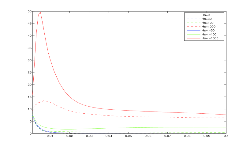
5 Numerical experiments

In order to carry out physically relevant experiments, the initial fields 𝒎0subscript𝒎0\boldsymbol{m}_{0}, 𝑯0subscript𝑯0\boldsymbol{H}_{0} must satisfy condition (2.2). This can be achieved by taking

𝑯0=𝑯0χD𝒎0,subscript𝑯0superscriptsubscript𝑯0subscript𝜒𝐷subscript𝒎0\boldsymbol{H}_{0}=\boldsymbol{H}_{0}^{*}-\chi_{D}\boldsymbol{m}_{0},

where div𝑯0=0divsuperscriptsubscript𝑯00\operatorname{{div\/}}\boldsymbol{H}_{0}^{*}=0 in D~~𝐷\widetilde{D}. In our experiment, for simplicity, we choose 𝑯0superscriptsubscript𝑯0\boldsymbol{H}_{0}^{*} to be a constant. We solve an academic example with D=D~=(0,1)3𝐷~𝐷superscript013D=\widetilde{D}=(0,1)^{3} and

𝒎0(𝒙)subscript𝒎0𝒙\displaystyle\boldsymbol{m}_{0}(\boldsymbol{x}) ={(0,0,1),|𝒙|12,(2𝒙A,A2|𝒙|2)/(A2+|𝒙|2),|𝒙|12,absentcases001superscript𝒙122superscript𝒙𝐴superscript𝐴2superscriptsuperscript𝒙2superscript𝐴2superscriptsuperscript𝒙2superscript𝒙12\displaystyle=\begin{cases}(0,0,-1),&\quad|\boldsymbol{x}^{*}|\geq\frac{1}{2},\\ (2\boldsymbol{x}^{*}A,A^{2}-|\boldsymbol{x}^{*}|^{2})/(A^{2}+|\boldsymbol{x}^{*}|^{2}),&\quad|\boldsymbol{x}^{*}|\leq\frac{1}{2},\end{cases}
𝑯0(𝒙)superscriptsubscript𝑯0𝒙\displaystyle\boldsymbol{H}_{0}^{*}(\boldsymbol{x}) =(0,0,Hs),𝒙D~,formulae-sequenceabsent00subscript𝐻𝑠𝒙~𝐷\displaystyle=(0,0,H_{s}),\quad\boldsymbol{x}\in\widetilde{D},

where 𝒙=(x1,x2,x3)𝒙subscript𝑥1subscript𝑥2subscript𝑥3\boldsymbol{x}=(x_{1},x_{2},x_{3}), 𝒙=(x10.5,x20.5,0)superscript𝒙subscript𝑥10.5subscript𝑥20.50\boldsymbol{x}^{*}=(x_{1}-0.5,x_{2}-0.5,0) and A=(12|𝒙|)4/4𝐴superscript12superscript𝒙44A=(1-2|\boldsymbol{x}^{*}|)^{4}/4. The constant Hssubscript𝐻𝑠H_{s} represents the strength of 𝑯0subscript𝑯0\boldsymbol{H}_{0} in the x3subscript𝑥3x_{3}-direction. We compute the experiments for Hs=0subscript𝐻𝑠0H_{s}=0, ±30plus-or-minus30\pm 30, ±100plus-or-minus100\pm 100 and ±1000plus-or-minus1000\pm 1000. We set the values for the other parameters in (1.1) and (1.2) as λ1=λ2=μ0=σ=1subscript𝜆1subscript𝜆2subscript𝜇0𝜎1\lambda_{1}=\lambda_{2}=\mu_{0}=\sigma=1.

The domain D𝐷D is partitioned into uniform cubes with the mesh size h=1/231superscript23h=1/2^{3}, where each cube consists of six tetrahedra. We choose the time step k=103𝑘superscript103k=10^{-3} and the parameter θ𝜃\theta in Algorithm 2.1 to be 0.70.70.7. The construction of the basis functions for 𝕎h(j)superscriptsubscript𝕎𝑗\mathbb{W}_{h}^{(j)} and 𝕐hsubscript𝕐\mathbb{Y}_{h} in this algorithm is discussed in [13]. At each iteration we need to solve a linear system of size (2N+M)×(2N+M)2𝑁𝑀2𝑁𝑀(2N+M)\times(2N+M), recalling that N𝑁N is the number of vertices and M𝑀M is the number of edges in the triangulation. The code is written in Fortran90.

The evolution of 𝒎h,kDsubscriptnormsubscript𝒎𝑘𝐷\|\nabla\boldsymbol{m}_{h,k}\|_{D}, 𝑯h,kD~subscriptnormsubscript𝑯𝑘~𝐷\|\boldsymbol{H}_{h,k}\|_{\widetilde{D}} and ×𝑯h,kD~subscriptnormsubscript𝑯𝑘~𝐷\|\nabla\times\boldsymbol{H}_{h,k}\|_{\widetilde{D}} are depicted in Figures 1, 2 and 3, respectively. Figure 4 shows that the solution satisfies condition (2.6) in Definition 2.1.

Refer to caption
Figure 1: Plot of t𝒎h,k(t)Dmaps-to𝑡subscriptnormsubscript𝒎𝑘𝑡𝐷t\mapsto\|\nabla\boldsymbol{m}_{h,k}(t)\|_{D} .
Refer to caption
Figure 2: Plot of t𝑯h,k(t)D~maps-to𝑡subscriptnormsubscript𝑯𝑘𝑡~𝐷t\mapsto\|\boldsymbol{H}_{h,k}(t)\|_{\widetilde{D}} .
Refer to caption
Figure 3: Plot of t×𝑯h,k(t)D~maps-to𝑡subscriptnormsubscript𝑯𝑘𝑡~𝐷t\mapsto\|\nabla\times\boldsymbol{H}_{h,k}(t)\|_{\widetilde{D}} .
Refer to caption
Figure 4: Plot of logt(t)maps-to𝑡𝑡\log t\mapsto{\cal E}(t)
Remark 5.1.

By the time this paper was written up, we learnt that Baňas, Page and Praetorius [4] independently solved a similar problem. They also used a linear scheme similar to our scheme, even though their variational formulation was different.

References

  • [1] F. Alouges. A new finite element scheme for Landau-Lifchitz equations. Discrete Contin. Dyn. Syst. Ser. S, 1(2):187–196, 2008.
  • [2] L. Baňas, S. Bartels, and A. Prohl. A convergent implicit finite element discretization of the Maxwell–Landau–Lifshitz–Gilbert equation. SIAM J. Numer. Anal., 46(3):1399–1422, 2008.
  • [3] S. Bartels. Stability and convergence of finite-element approximation schemes for harmonic maps. SIAM J. Numer. Anal., 43(1):220–238 (electronic), 2005.
  • [4] L. Baňas, M. Page, and D. Praetorius. A convergent linear finite element scheme for the Maxwell–Landau–Lifshitz–Gilbert equation. Submitted, 2012.
  • [5] D. Braess. Finite Elements. Cambridge University Press, Cambridge, third edition, 2007. Theory, fast solvers, and applications in elasticity theory, Translated from the German by Larry L. Schumaker.
  • [6] Z. Chen. Finite Element Methods and Their Applications. Scientific Computation. Springer-Verlag, Berlin, 2005.
  • [7] I. Cimrák. Error analysis of a numerical scheme for 3D Maxwell–Landau–Lifshitz system. Math. Methods Appl. Sci., 30(14):1667–1683, 2007.
  • [8] I. Cimrák. Existence, regularity and local uniqueness of the solutions to the Maxwell–Landau–Lifshitz system in three dimensions. J. Math. Anal. Appl., 329(2):1080–1093, 2007.
  • [9] T. Gilbert. A Lagrangian formulation of the gyromagnetic equation of the magnetic field. Phys Rev, 100:1243–1255, 1955.
  • [10] B. Guo and S. Ding. Landau–Lifshitz Equations, volume 1 of Frontiers of Research with the Chinese Academy of Sciences. World Scientific Publishing Co. Pte. Ltd., Hackensack, NJ, 2008.
  • [11] C. Johnson. Numerical Solution of Partial Differential Equations by the Finite Element Method. Cambridge University Press, Cambridge, 1987.
  • [12] L. Landau and E. Lifschitz. On the theory of the dispersion of magnetic permeability in ferromagnetic bodies. Phys Z Sowjetunion, 8:153–168, 1935.
  • [13] K.-N. Le and T. Tran. A finite element approximation for the quasi-static Maxwell–Landau–Lifshitz–Gilbert equations. Submitted ANZIAM J. 2012.
  • [14] P. Monk. Finite Element Methods for Maxwell’s equations. Numerical Mathematics and Scientific Computation. Oxford University Press, New York, 2003.