Systematic variations in divergence angle

Abstract

Practical methods for quantitative analysis of radial and angular coordinates of leafy organs of vascular plants are presented and applied to published phyllotactic patterns of various real systems from young leaves on a shoot tip to florets on a flower head. The constancy of divergence angle is borne out with accuracy of less than a degree. It is shown that apparent fluctuations in divergence angle are in large part systematic variations caused by the invalid assumption of a fixed center and/or by secondary deformations, while random fluctuations are of minor importance.

1 Introduction

It has long since been recognized that divergence angles between successive leafy organs of vascular plants are accurately regulated at one of special constant values. Deviations from the the constant angle are normally so small that this botanical phenomenon, phyllotaxis, should rather be regarded as a genuine subject of exact science. Besides the angular regularity, radial coordinates also exhibit mathematical regularity.

In a polar coordinate system, position of the $n$-th leaf is specified by the radial and angular coordinates $(r_{n},\theta_{n})$. The angular regularity is expressed by the equation

$$\theta_{n}=nd,$$ (1)

where $d$ is a divergence angle. A spiral pattern is made when the radial component $r_{n}$ is a monotonic function of $n$, i.e., $r_{n}$ preserves the order of the leaf index $n$. Particularly important is a logarithmic spiral given by

$$r_{n}=a^{n},$$ (2)

where $a$ is a constant, called the plastochron ratio. Leaf primordia at a shoot tip appear to be arranged on a logarithmic spiral. Eq. (2) is a solution of the differential equation of exponential growth,

$$\frac{{\rm d}}{{\rm d}n}\log r_{n}=\log a.$$ (3)

Thus, the logarithmic spiral is characterized by the constant growth rate $\log a$. On the other side, a power-law spiral given by

$$r_{n}=\sqrt{n}$$ (4)

has been often used as a mathematical model of packed seeds on a sunflower head (Vogel (1979); Ridley (1982); Rivier et al. (1984)). The equation (4) is expected when all seeds have equal areas, i.e., for the area per seed,

$$\frac{{\rm d}}{{\rm d}n}(\pi r_{n}^{2})={\rm const}.$$ (5)

In mathematical studies, the relations (1), (2) and (4) are often accepted without inquiring their empirical basis. From a physical standpoint, the validity of the mathematical relations has to be checked against experiments at all events. While embarking on quantitative assessment, however, we are confronted with a serious methodological problem. First of all, a center of the pattern, the origin of the polar coordinate system, must be located. Unfortunately, it is not always possible to locate a fixed center properly and objectively. The uncertainty of the central position becomes a fundamental obstacle to assessing the empirical relations in a quantitative manner.

Quantitative analysis of phyllotaxis has not been made until recently. Maksymowych and Erickson (1977) used a trigonometric method for evaluating divergence angle from positions of three successive leaves. Their three-point method is based on the exponential growth (2), and it has been developed by Meicenheimer (1986) and Hotton (2003). On the other side, Rutishauser (1998) has estimated the plastochron ratio $a$ from the geometrical mean $({r_{m}}/{r_{n}})^{1/(m-n)}$ evaluated for selected leaves. The exponential growth is verified by the observation that the mean is nearly constant. Ryan et al. (1991) has assessed the validity of (4) for real sunflowers by indirect means of evaluating the Euclidean distance between successive seeds, $D_{n}^{2}=r_{n}^{2}+r_{n+1}^{2}-2r_{n}r_{n+1}\cos(\theta_{n}-\theta_{n+1})$. This method has a merit of being independent of the choice of the center position. They have attempted parameter fittings with various functional forms of $r_{n}$. Matkowski et al. (1998) has investigated computational methods by regarding the center of gravity as the center of the pattern. Hotton (2003) has proposed to use the minimal variation center that minimizes the standard deviation of divergence angles.

The main aim of this paper is to present practical methods for evaluating radial and angular coordinates of phyllotactic units without assuming any specific functional form of $r_{n}$ nor the existence of a fixed center of the pattern. In Sec. 2.1, a floating center of divergence is defined by positions of four consecutive leaves. In Sec. 2.2, a floating center of parastichy is defined by four nearby points forming a unit cell of a parastichy lattice. For this purpose, a systematic index system for leaves of a multijugate pattern is proposed in Sec. 2.2.2. In Sec. 3, effects of uniform deformation are considered. In Sec. 4, presented methods are applied to real representative systems, which are arbitrarily chosen from previous works (Maksymowych and Erickson (1977); Ryan et al. (1991); Rutishauser (1998); Hotton et al. (2006)). In A, mathematical characteristics of the logarithmic spiral pattern are examined carefully. To assist in interpreting the results in Sec. 4, general mathematical formulas for the plastochron ratio $a$ of systems with orthogonal parastichies are derived. In B, a practical method for numbering packed florets of a high phyllotaxis pattern is presented. The method is based on a number theoretic algorithm. To analyze phyllotaxis of Asteraceae, Hotton et al. (2006) have introduced a primordia front based on the assumption that the pattern has a definite center and the radius $r_{n}$ from the center is a monotonic function of $n$. In B, a similar concept, a front circle on a parastichy lattice, is introduced without referring to the center.

2 Floating center

2.1 Floating center of divergence

For the purpose of this paper, it is suffice to investigate phyllotactic patterns projected on a plane. For three-dimensional analysis, see Hotton et al. (2006) and references therein. An effect due to a slight inclination of the normal axis is discussed in Sec. 3.

Figure 1: Given four consecutive points, $P_{1}$, $P_{2}$, $P_{3}$ and $P_{4}$, a center of divergence $O_{23}$ is defined such that $\angle P_{1}O_{23}P_{2}=\angle P_{2}O_{23}P_{3}=\angle P_{3}O_{23}P_{4}$. A dashed curve $C_{2}$ is a locus of the point $O_{2}$ satisfying $\angle P_{1}O_{2}P_{2}=\angle P_{2}O_{2}P_{3}$. Similarly, a dashed curve $C_{3}$ is drawn by the point $O_{3}$ satisfying $\angle P_{2}O_{3}P_{3}=\angle P_{3}O_{3}P_{4}$. The point where $C_{2}$ and $C_{3}$ intersect is $O_{23}$, the floating center of divergence.

Consider four consecutive points $P_{1}$, $P_{2}$, $P_{3}$ and $P_{4}$ in the same geometric plane. Given the first three points $P_{1}$, $P_{2}$ and $P_{3}$, the point $O_{2}$ satisfying

$$\angle P_{1}O_{2}P_{2}=\angle P_{2}O_{2}P_{3}$$ (6)

defines a curve $C_{2}$ (Fig. 1). When $P_{2}P_{1}=P_{2}P_{3}$, or the triangle $P_{1}P_{2}P_{3}$ is isosceles, $C_{2}$ bisects the vertex angle $\angle P_{1}P_{2}P_{3}$. Similarly, for the three points $P_{2}$, $P_{3}$ and $P_{4}$, we obtain a curve $C_{3}$ traced by the point $O_{3}$ satisfying

$$\angle P_{2}O_{3}P_{3}=\angle P_{3}O_{3}P_{4}.$$ (7)

The floating center of divergence $O_{23}$ is defined as the crossing point of the two curves $C_{2}$ and $C_{3}$. By definition,

$$\angle P_{1}O_{23}P_{2}=\angle P_{2}O_{23}P_{3}=\angle P_{3}O_{23}P_{4}.$$

Thus, the three angles spanned by the four consecutive points define a divergence angle,

$$d_{2}\equiv\angle P_{2}O_{23}P_{3}.$$ (8)

Distance from $O_{23}$ is denoted as

$$r_{2}\equiv|\overrightarrow{O_{23}P_{2}}|.$$

In general, the divergence angle $d_{n}$ and the radius $r_{n}$ are evaluated from four consecutive points $P_{n-1}$, $P_{n}$, $P_{n+1}$ and $P_{n+2}$;

$$d_{n}\equiv\angle P_{n}O_{nn+1}P_{n+1},$$ (9)

$$r_{n}\equiv|\overrightarrow{O_{nn+1}P_{n}}|.$$ (10)

These quantities are compared with

$$d_{n}^{(0)} = \angle P_{n}O_{0}P_{n+1},$$ (11)

and

$$r_{n}^{(0)}=|\overrightarrow{O_{0}P_{n}}|,$$ (12)

which are defined in terms of an arbitrarily chosen center $O_{0}$.

Given coordinates of the four points $P_{n}$ $(n=1,2,3,4)$, the position of the floating center $O_{23}$ is parametrically represented by means of two parameters $X$ and $Y$;

$$\overrightarrow{P_{2}O_{23}}=X\overrightarrow{P_{2}P_{3}}+Y\overrightarrow{P_{2}P_{1}}.$$ (13)

The two parameters are determined by the two equations (6) and (7), namely

$$\frac{|\overrightarrow{O_{23}P_{1}}|^{2}+|\overrightarrow{O_{23}P_{2}}|^{2}-|\overrightarrow{P_{1}P_{2}}|}{|\overrightarrow{O_{23}P_{1}}||\overrightarrow{O_{23}P_{2}}|}=\frac{|\overrightarrow{O_{23}P_{2}}|^{2}+|\overrightarrow{O_{23}P_{3}}|^{2}-|\overrightarrow{P_{2}P_{3}}|}{|\overrightarrow{O_{23}P_{2}}||\overrightarrow{O_{23}P_{3}}|},$$ (14)

and

$$\frac{|\overrightarrow{O_{23}P_{2}}|^{2}+|\overrightarrow{O_{23}P_{3}}|^{2}-|\overrightarrow{P_{2}P_{3}}|}{|\overrightarrow{O_{23}P_{2}}||\overrightarrow{O_{23}P_{3}}|}=\frac{|\overrightarrow{O_{23}P_{3}}|^{2}+|\overrightarrow{O_{23}P_{4}}|^{2}-|\overrightarrow{P_{3}P_{4}}|}{|\overrightarrow{O_{23}P_{3}}||\overrightarrow{O_{23}P_{4}}|}$$ (15)

by the cosine formula in trigonometry.

For example, consider vertex points $P_{n}$ ($n=1,2,3,4,5$) of a regular pentacle, whose Cartesian coordinates are given by $(x_{n},y_{n})=(\cos nd,\sin nd),$ where $d=2\pi\alpha$ in radians and $\alpha=\frac{2}{5}$. Let the center $O_{23}$ of the four points $P_{n}$ ($n=1,2,3,4$) be represented as (13). For this special case, it is not difficult to find the solution $X=Y=\frac{1}{2+\tau}\simeq 0.2764$ by geometrical considerations. The golden ratio

$$\tau=\frac{\sqrt{5}+1}{2}$$ (16)

is the irrational number quintessential to the phenomenon of phyllotaxis. The estimate of $X\simeq Y\sim 0.3$ can be used as an initial guess for the numerical search of solutions in general cases.

The manner in which the floating center floats around may be illustrated by means of a line segment connecting the floating center and the middle point of the middle two leaves defining the center, that is, the line segment $O_{23}M_{23}$, where $M_{23}$ is the middle point of $P_{2}$ and $P_{3}$. Let us call a graph of the line segments a divergence diagram. If the center is fixed in space, all the line segments radiate from the fixed center. If it is not, the lines cross with each other. See Fig. 4, for instance.

When a pattern with small divergence angles is deformed significantly, it may happen that no center is defined because the two curves $C_{2}$ and $C_{3}$ do not cross (Fig. 2). Even in such a case, a center can be defined formally by selecting four points properly. Here it is remarked only that a pattern consisting of more than three points may not have a definite center. In other words, it is very special for numerous leaves comprising a phyllotactic pattern to have a unique, fixed center. Assuming the fixed center is not at all a trivial matter.

Figure 2: Four points $P_{i}$ ($i=1,2,3,4$) from a deformed Lucas pattern for which two curves $C_{2}$ and $C_{3}$ as defined in Fig. 1 fail to cross. Thus, it may happen that the center of divergence is not defined when divergence angle is small and variable.

2.2 Floating center of parastichy

2.2.1 Spiral phyllotaxis

Figure 3: From four nearby points $P_{n}$, $P_{n+q}$, $P_{n+q^{\prime}}$ and $P_{n+q+q^{\prime}}$ making a tetragonal cell of a lattice of $q$ and $q^{\prime}$ parastichies, a center of parastichy $O_{n}^{(q,q^{\prime})}$ is determined by (17) and (18). By definition, four angles subtended by four sides of the tetragon give a unique divergence angle against $O_{n}^{(q,q^{\prime})}$, which is called the floating center of parastichy.

For a spiral pattern with one leave per each node, leaves are orderly indexed by an integer $n$, called the plastochron. Four points for a center need not be consecutive in plastochron. A divergence angle is evaluated from four vertex points $P_{n}$, $P_{n+q}$, $P_{n+q^{\prime}}$ and $P_{n+q+q^{\prime}}$ of a unit cell of a parastichy lattice, where $q$ and $q^{\prime}$ are opposite parastichy numbers. Parastichies of logarithmic spirals are discussed in A, where it is shown that divergence angle $d=2\pi\alpha_{0}$ of an ideal pattern satisfies the inequalities (56) in terms of two auxiliary integers $p$ and $p^{\prime}$ satisfying $pq^{\prime}-p^{\prime}q=1$, (57). With this in mind, a center of parastichy $O_{n}^{(q,q^{\prime})}$ is defined such that

$$q^{\prime}\angle P_{n}O_{n}^{(q,q^{\prime})}P_{n+q}+q\angle P_{n}O_{n}^{(q,q^{\prime})}P_{n+q^{\prime}}=2\pi,$$ (17)

and

$$\angle P_{n}O_{n}^{(q,q^{\prime})}P_{n+q}=\angle P_{n+q^{\prime}}O_{n}^{(q,q^{\prime})}P_{n+q+q^{\prime}}.$$ (18)

where $\angle P_{n}O_{n}^{(q,q^{\prime})}P_{n+q}$ signifies the angle subtended by line segments $O_{n}^{(q,q^{\prime})}P_{n}$ and $O_{n}^{(q,q^{\prime})}P_{n+q}$. See Fig. 3. Then, four angles made by the four points give a divergence angle;

$$d_{n}^{(q,q^{\prime})} = \left(2\pi p-\angle P_{n}O_{n}^{(q,q^{\prime})}P_{n+q}\right)/q$$ (19)

$$= \left(2\pi p-\angle P_{n+q^{\prime}}O_{n}^{(q,q^{\prime})}P_{n+q+q^{\prime}}\right)/q$$

$$= \left(\angle P_{n}O_{n}^{(q,q^{\prime})}P_{n+q^{\prime}}+2\pi p^{\prime}\right)/q^{\prime}$$

$$= \left(\angle P_{n+q}O_{n}^{(q,q^{\prime})}P_{n+q+q^{\prime}}+2\pi p^{\prime}\right)/q^{\prime}.$$

The rationale behind this definition may be understood by expressing the first equation as $\angle P_{n}O_{n}^{(q,q^{\prime})}P_{n+q}=2\pi p-d_{n}^{(q,q^{\prime})}q$, which is to be compared with the denominator of (50). This is the net angle between the two successive points along a $q$ parastichy $P_{n}$ and $P_{n+q}$ when divergence angles between the two points are equal to $d_{n}^{(q,q^{\prime})}$. The difference in the signs in front of geometrical angles like $\angle P_{n}O_{n}^{(q,q^{\prime})}P_{n+q}$ in (19) is due to the convention that the angles including $d_{n}^{(q,q^{\prime})}$ are regarded as positive quantities.

Coordinates of the center $O_{n}^{(q,q^{\prime})}$ are represented in terms of two parameters $r$ and $\theta$ as

$$\overrightarrow{P_{n}O_{n}^{(q,q^{\prime})}}=r\cos\theta\overrightarrow{P_{n+q}P_{n}}+r\sin\theta\overrightarrow{P_{n+q^{\prime}}P_{n}}.$$ (20)

Accordingly, (17) and (18) are regarded as the defining equations for $r$ and $\theta$. As is clear from Fig. 3, it is generally assumed that $r>0$ and $0<\theta<\frac{\pi}{2}$. By regarding $\theta$ as a given constant, the first equation (17) determines $r$ for the given value of $\theta$, or $r$ is determined as a function of $\theta$. Then, the parameter $\theta$ is fixed by the second equation (18). Thus, the center $O_{n}^{(q,q^{\prime})}$ for given $P_{n}$, $P_{n+q}$, $P_{n+q^{\prime}}$ and $P_{n+q+q^{\prime}}$ is fixed numerically. The equations depend not only on the coordinates of the four points, but also on the parastichy numbers $q$ and $q^{\prime}$, while either $p$ or $p^{\prime}$ is needed to evaluate the divergence angle in (19).

A caveat: In the above, it is assumed that $P_{n}$ with the smallest index $n$ is positioned nearest to the center (Fig. 3). In the opposite convention, $P_{n}$ is farther from the center than $P_{n+q+q^{\prime}}$. To adapt the above results to this case, the four points $P_{n}$, $P_{n+q}$, $P_{n+q^{\prime}}$ and $P_{n+q+q^{\prime}}$ should be replaced by $P_{n+q+q^{\prime}}$, $P_{n+q^{\prime}}$, $P_{n+q}$ and $P_{n}$, respectively. A set of equations (17), (18), and (19) is invariant by this replacement, whereas (20) should be read as

$$\overrightarrow{P_{n+q+q^{\prime}}O_{n}^{(q,q^{\prime})}}=r\sin\theta\overrightarrow{P_{n+q}P_{n+q+q^{\prime}}}+r\cos\theta\overrightarrow{P_{n+q^{\prime}}P_{n+q+q^{\prime}}}.$$ (21)

In the biological literature, leaves on a stem are numbered in the order of appearance, while primordia on an apex are counted in the opposite order.

While $d_{n}$ in (9) based on four distant points is insensitive to individual displacements of the points, $d_{n}^{(q,q^{\prime})}$ in (19) based on nearby points is insensitive to a collective displacement of the points. The latter has a merit of wider applicability in practice. It is stressed again that parastichies generally do not have a definite center; the center $O_{n}^{(q,q^{\prime})}$ thus determined depends on the plastochron $n$ and the parastichy pair $(q,q^{\prime})$.

2.2.2 Multijugate phyllotaxis

A multijugate pattern bears more than one leaves at each node. There has been no established way of systematize multijugate leaves, particularly because a special index to distinguish leaves at a node is lacking. Therefore, in the first place, a systematic index system for a multijugate pattern is proposed below. Then, the center of parastichy is defined similarly as in the last subsection.

A $J$-jugate pattern has $J$ leaves at a node. There are $J$ fundamental spirals correspondingly. Each of $J$ leaves at the $n$-th node is specified by polar coordinates $(r_{n,j},\theta_{n,j})$, where the jugacy index $j=0,1,2,\cdots,J-1$ is introduced. Any leaf may be chosen as the origin $(n,j)=(0,0)$ of the index system. Along with the plastochron $n$, the jugacy index $j$ is set in order in the direction of the fundamental spirals. The leaf with the index $(n,j)$ is referred to by the symbol $P_{n}^{j}$, or simply denoted as $n^{j}$. For instance, see Fig. 13 for a trijugate system with $J=3$. For convenience’ sake, the value range of the jugacy index $j$ is extended to all integers; the coordinates $(r_{n,j},\theta_{n,j})$ are regarded as periodic in $j$ with period of $J$, namely $(r_{nj+J},\theta_{nj+J})=(r_{n,j},\theta_{n,j})$ for all $n$ and $j$. Accordingly, divergence angle

$$d_{n}^{j}=\theta_{n+1,j}-\theta_{n,j}$$ (22)

is periodic in $j$. As implied by the notation, $d_{n}^{j}$ depends on the leaf index $(n,j)$, whereas it becomes constant, $d_{n}^{j}=d$, for an ideal pattern.

To put it concretely, let us consider an ideal multijugate system spiraling in the positive direction, i.e., $d>0$. A pattern with a negative angle $d<0$ is the mirror image of the positive counterpart. In an ideal $J$-jugate pattern, the radial coordinate $r_{n}^{j}$ is independent of the jugacy index $j$,

$$r_{n,j}=r_{n},$$

whereas the angular coordinate is given by

$$\theta_{n,j}=2\pi\left(n\alpha_{0}+\frac{j}{J}\right),$$ (23)

where the divergence angle $d=2\pi\alpha_{0}$ is represented with a dimensionless parameter $\alpha_{0}$. Without loss of generality, $0<J\alpha_{0}<\frac{1}{2}$. For multijugate patterns $J>1$, the other quantity of interest is displacement angle between neighboring leaves at a node,

$$\Delta_{n}^{j}=\theta_{n,j+1}-\theta_{n,j}-\frac{2\pi}{J}.$$ (24)

For the ideal pattern with (23), $\Delta_{n}^{j}=0$. In general, $\Delta_{n}^{j}$ fluctuates evenly about zero.

In this index system, a parastichy is specified by a set of numbers $(q,j)$, increments of $(n,j)$. Conspicuous parastichies following nearby leaves are shown to have $j=-p$, where $p$ is an integer near $J\alpha_{0}q$ (cf. below (50)). Thus, the $q$ parastichy running through a leaf $P_{n}^{i}$ connects the points $P_{n}^{i}$, $P_{n+q}^{i-p}$, $P_{n+2q}^{i-2p}$, $P_{n+3q}^{i-3p},\cdots$. For instance, the trijugate pattern in Fig. 13 has $J=3$ and $(q,p)=(3,1)$, $(5,2)$, etc. Note that a 3-parastichy $1^{0}-4^{-1}-7^{-2}-10^{-3}-\cdots$ is equivalently represented as $1^{0}-4^{2}-7^{1}-10^{0}-\cdots$, as the jugacy superscript $j$ is understood modulo $J=3$ by the periodic extension prescribed above.

Having thus prepared, the method of the parastichy center in the last subsection is applied. The divergence angle $d_{n}^{j(q,q^{\prime})}$ of a multijugate system is defined by the four points $P_{n}^{j}$, $P_{n+q}^{j-p}$, $P_{n+q^{\prime}}^{j-p^{\prime}}$, $P_{n+q+q^{\prime}}^{j-p-p^{\prime}}$; (17), (18) and (19) should read

$$q^{\prime}\angle P_{n}^{j}O_{n}^{(q,q^{\prime})}P_{n+q}^{j-p}+q\angle P_{n}^{j}O_{n}^{(q,q^{\prime})}P_{n+q^{\prime}}^{j-p^{\prime}}=2\pi/J,$$ (25)

$$\angle P_{n}^{j}O_{n}^{(q,q^{\prime})}P_{n+q}^{j-p}=\angle P_{n+q^{\prime}}^{j-p^{\prime}}O_{n}^{(q,q^{\prime})}P_{n+q+q^{\prime}},$$ (26)

and

$$d_{n}^{j(q,q^{\prime})} = \left(\frac{2\pi p}{J}-\angle P_{n}^{j}O_{n}^{(q,q^{\prime})}P_{n+q}^{j-p}\right)/q$$ (27)

$$= \left(\frac{2\pi p}{J}-\angle P_{n+q^{\prime}}^{j-p^{\prime}}O_{n}^{(q,q^{\prime})}P_{n+q+q^{\prime}}^{j-p-p^{\prime}}\right)/q$$

$$= \left(\angle P_{n}^{j}O_{n}^{(q,q^{\prime})}P_{n+q^{\prime}}^{j-p^{\prime}}+\frac{2\pi p^{\prime}}{J}\right)/q^{\prime}$$

$$= \left(\angle P_{n+q}^{j-p}O_{n}^{(q,q^{\prime})}P_{n+q+q^{\prime}}^{j-p-p^{\prime}}+\frac{2\pi p^{\prime}}{J}\right)/q^{\prime}.$$

3 Effect of uniform deformation

Consider a regular spiral pattern in which position of the $n$-th leaf is given by Cartesian coordinates $(x_{n},y_{n})$. The center $O_{0}$ of the polar coordinate system $(r_{n}^{(0)},\theta_{n}^{(0)})$ is set at the origin. The azimuthal angle $\theta_{n}^{(0)}$ is measured from the $x$-axis. As typical cases for a phyllotactic pattern to lose track of the center, two types of global deformation are considered. The deformation is characterized by a single parameter representing strain $C$.

Uniform deformation of the first order transforms $(x_{n},y_{n})$ as follows;

$$x_{n} \longrightarrow \left\{\begin{array}[]{ll}(1+C_{1})x_{n}.&x_{n}\geq 0\\ (1-C_{1})x_{n}.&x_{n}<0\\ \end{array}\right.$$ (30)

$$y_{n} \longrightarrow y_{n}.$$ (31)

Uniform deformation of the second order makes

$$x_{n} \longrightarrow (1-C_{2})x_{n},$$

$$y_{n} \longrightarrow y_{n}.$$ (32)

The magnitude of deformation is represented by constants $C_{1}$ and $C_{2}$, respectively, which are assumed significantly smaller than 1. In both cases, the radial component $r_{n}^{(0)}\equiv\sqrt{x_{n}^{2}+y_{n}^{2}}$ and divergence angle $\theta_{n}^{(0)}-\theta_{n-1}^{(0)}$ suffer modulation periodic in the azimuthal angle $\theta_{n}^{(0)}$. The periods of modulation for the first and the second order deformation are 360 and 180 degrees, respectively.

The amplitude of modulation in the radius $r_{n}^{(0)}\pm\Delta r_{n}^{(0)}$ is given by

$$\frac{\Delta r_{n}^{(0)}}{{r_{n}^{(0)}}}=C_{1}$$ (33)

for the first order deformation, and

$$\frac{\Delta r_{n}^{(0)}}{{r_{n}^{(0)}}}=\frac{C_{2}}{2}$$ (34)

for the second order deformation.

Amplitude of modulation in divergence angle, ${\Delta d}^{(0)}$, may be estimated as follows. Consider an isosceles triangle with the vertex angle $d^{(0)}$, the base of length $2L$, and the height $H$. Then,

$$\tan\frac{d^{(0)}}{2}=\frac{L}{H}.$$

By the first order deformation, $d^{(0)}$ becomes $d^{(0)}\pm\Delta d^{(0)}$ when the height $H$ parallel to the $x$ axis is modified to $(1\mp C_{1})H$. By the second order deformation, $d$ is modified to $d^{(0)}\pm\Delta d^{(0)}$ as $(H,L)$ become $((1-C_{2})H,L)$ and $(H,(1-C_{2})L)$. In either case,

$$\tan\frac{d^{(0)}\pm\Delta d^{(0)}}{2}\simeq\frac{L}{H}(1\mp C),$$ (35)

where $C$ is $C_{1}$ or $C_{2}$. Accordingly,

$${\Delta d^{(0)}}\simeq C{\sin d^{(0)}}.$$ (36)

In particular,

$${\Delta d^{(0)}}\simeq 38.7C\ {\rm degrees}$$ (37)

for $d^{(0)}=137.5$ degrees, and

$${\Delta d^{(0)}}\simeq 56.5C\ {\rm degrees}$$ (38)

for $d^{(0)}=99.5$ degrees.

The first order deformation may be caused by a tendency toward or against the direction of the sun (Kumazawa and Kumazawa (1971)). The second order deformation may be caused by various reasons, real or apparent. The most possible would be due to uniform compression. It applies also to the case where a pattern is observed from a direction oblique to the perpendicular direction. If the angle of inclination is denoted as $\varphi$ in radian measure, then $1-C_{2}=\cos\varphi$, or $C_{2}\simeq{\varphi^{2}}/{2}$.

4 Results

4.1 Example

Figure 4: An ideal pattern of a logarithmic spiral with the plastochron ratio $a=1.073$ is compressed (a) by (31) with $C_{1}=0.05$, and (b) by (32) with $C_{2}=0.05$. Leaves are represented with points with integer index $n$. Radiating lines represent $O_{nn+1}M_{nn+1}$, where $O_{nn+1}$ is the floating center of divergence for the four consecutive leaves from the $(n-1)$-th to $(n+2)$-th leaves and $M_{nn+1}$ is the middle point of the $n$-th and $(n+1)$-th leaves. It is called a divergence diagram in Sec. 2.1.

(a) $d^{(0)}$ and $d$ against $n$

(b) $r^{(0)}$ and $r$ against $n$

(c) $d^{(0)}$ and $d$ against $\theta$

(d) $\Delta r^{(0)}/r^{(0)}$ and $\Delta r/r$ against $\theta$

Figure 5: Results for the deformed pattern in Fig. 4. $d^{(0)}$ and $r^{(0)}$ are divergence angle and radial coordinate with respect to the center of the original (undeformed) spiral pattern, while $d$ and $r$ are divergence angle and radial coordinate with respect to the floating center of divergence. For the horizontal axis, $n$ is the leaf index, and $\theta$ is the polar angle, or azimuth. $\Delta r^{(0)}$ and $\Delta r$ are changes in $r^{(0)}$ and $r$ by the uniform deformation for $C_{1}=0.05$.

(a) $d^{(0)}$ and $d$ against $n$

(b) $r^{(0)}$ and $r$ against $n$

(c) $d^{(0)}$ and $d$ against $\theta$

(d) $\Delta r^{(0)}/r^{(0)}$ and $\Delta r/r$ against $\theta$

Figure 6: Results for the deformed pattern in Fig. 4 ($C_{2}=0.05$); cf. Fig. 5.

Figure 7: Divergence angles of the original (not deformed) pattern of Fig. 4 are measured against a misplaced center $O_{0}$ set at the middle point of leaves 1 and leaf 5. The misplacement brings about apparent wild variations in $d_{n}^{(0)}$ (open circles, left), which are correlated with azimuth $\theta_{n}$ (right). Divergence angle $d_{n}$ evaluated with the floating center of divergence (filled circles) does not depend on the wrong center $O_{0}$; the original divergence angle is correctly retrieved without knowing the true center.

Consider a regular pattern with $d=2\pi/\tau^{2}$ (137.5 degrees) and $a=1.073$ for (1) and (2). This is an orthogonal $(5,8)$ system corresponding to $i=5$ in (69). By deforming the pattern according to (31) with $C_{1}=0.05$ and (32) with $C_{2}=0.05$, patterns shown in Figs. 4 and 4 are obtained, respectively. In Fig. 4, line segments radiating from the center represent the divergence diagram explained at the end of Sec. 2.1. The fixed center $O_{0}$ for divergence angle $d^{(0)}$ and radius $r^{(0)}$ is set at the center of the original pattern. Divergence angles $d^{(0)}$, $d$ and radii $r^{(0)}$, $r$ for the pattern of Figs. 4 and 4 are shown in Figs. 5 and 6, respectively. All quantities show characteristic variations. A type of variations as exhibited by $d^{(0)}$ in Fig. 5(a) is frequently met in real systems. Fig. 5(c) shows that the variations are correlated with azimuth $\theta_{n}$. In general, deformation has a larger effect on the divergence angles than on the radii. Variations in the divergence angle $d$ by means of the floating center in Sec. 2.1 are considerably suppressed compared with those of $d^{(0)}$. A period of 180 degrees in Fig. 6(c) is the characteristic of uniform compression in one direction, namely deformation of the second order. Divergence angles facing the compressed direction increase apparently. For $C_{2}=0.05$, (37) gives $\Delta d\simeq 1.9$ degrees, which corresponds to the amplitudes of $d^{(0)}$ in Fig. 6(c) and $\Delta r^{(0)}/r^{(0)}$ in Fig. 6(d). The amplitudes of $d$ and $\Delta r/r$ are suppressed and enhanced compared with $d^{(0)}$ and $\Delta r^{(0)}/r^{(0)}$, respectively. The factors of suppression and enhancement are about the same value $\simeq 1.8$.

Even if a pattern has a definite center, misidentification of the center causes apparently systematic variations in $d^{(0)}$. Fig. 7 is a result for the undistorted pattern $C_{1}=C_{2}=0$, whereas the middle point of 1 and 5 is chosen as the nominal center $O_{0}$. The divergence $d$ based on the floating center does not depend on the choice of $O_{0}$, whereas the variations in $d^{(0)}$ exhibit a period of 360 degrees when plotted against the azimuth $\theta$. Thus, the misplacement of the center can be misinterpreted as the first order deformation.

These results indicate that systematic features of variations may not be revealed unless they are plotted against the azimuth.

4.2 Suaeda vera

(a) Position of leaves $(x_{n},y_{n})$

(b) Divergence angles $d_{n}$ and $d^{(0)}_{n}$ against the leaf index $n$

(c) $d_{n}$ and $d^{(0)}_{n}$ against $\theta_{n}$

(d) $\log r_{n}$ and $\log r^{(0)}_{n}$ against $n$

Figure 8: Results for a normal phyllotaxis of young leaves of Suaeda vera, whose pattern shown in (a) is taken after Fig. 1a of Rutishauser (1998). Radiating lines in (a) represent a divergence diagram (cf. the caption of Fig. 4 and Sec. 2.1).

As a typical example of real systems, phyllotaxis of young leaves of Suaeda vera is shown in Fig. 8(a) after Fig. 1a of Rutishauser (1998). The actual size of the pattern is about 1mm in diameter. Leaf position is optically read as marked in the original figure, which is a drawn figure based on a microtome section. A leaf is not a point. It has shape and size. In this case, and presumably in most past cases reported so far, position of a leaf is represented by the position of the main vascular bundle when it is visually discernible. This paper does not take up cases in which position of leaves may not be specified unambiguously. A fixed center $O_{0}$ for $d^{(0)}$ in Figs. 8(b) and 8(c) is set according to the original figure. Statistical results for divergence angle are $d^{(0)}=136.8\pm 5.8^{\circ}$ by the fixed center $O_{0}$, $d=136.9\pm 1.8^{\circ}$ by the floating center of divergence, and $d^{(5,8)}=137.0\pm 0.9^{\circ}$ by the floating center of parastichy. It is remarkable that no significant deviation from the ideal limit angle of $137.5^{\circ}$ is found, although the divergence diagram in Fig. 8(a) indicates that the pattern does not have a well-defined center. In the figures, $d_{n}^{(5,8)}$ for $n=15$ is omitted because no solution was found.

Rutishauser (1998) has remarked angular width of leaf arc, $i$, as another quantity of interest. From the original figure, it is estimated as $i=66\pm 13^{\circ}$. Oddly enough, the standard deviation of the angular width of leaf arc is larger than that of divergence angle. If the right tip of leaf arc is regarded as a representative point of the leaf, $d^{(0)}=137.4\pm 6.0^{\circ}$. If the left tip is used instead, $d^{(0)}=136.1\pm 5.8^{\circ}$. Thus, divergence angle does not depend on which part of leaf is regarded as a representative point. The results indicate that absolute positions of the leaves are not affected even though the angular width of each leaf arc fluctuates widely.

Apparent lack of stability in nominal divergence angle $d^{(0)}$ (open circles in Fig. 8(b)) is due to systematic variations of the type expected for the first order deformation (Fig. 8(c)). The azimuth plot of $d$ in Fig. 8(c) (closed circles) indicates a slight indication of peaks at $\theta\simeq 80^{\circ}$ and $\theta\simeq 80+180^{\circ}$, signifying deformation of the second order.

A semi-log plot of $r_{n}$ and $r_{n}^{(0)}$ in Fig. 8(d) confirms the exponential rule (2). Straight lines labeled with $(3,5)$, $(5,8)$ and $(8,13)$ represent the exponential growth according to (69) for $i=4,5$ and 6, respectively. In the original figure, leaves are in contact with each other along three contact parastichies 3, 5 and 8. The growth rate $\log a$ has to be estimated in order to evaluate the phyllotaxis index (P.I.) in (74). This may pose a methodological problem. The radial growth $r_{n}$ of a real system is neither continuous nor monotonic in $n$. There are systematic variations in $r_{n}^{(0)}$ and $r_{n}$, particularly because the pattern does not have a definite center. Accordingly, a bad method or a bad choice of leaves may give an unwanted result $\log a<0$ for some values of $n$. Rutishauser (1998) has evaluated $a\simeq 1.06$ based on two ratios for three leaves, namely 2, 18 and 31 in Fig. 8(a) (30, 14 and 1 in the original figure). In the presence of systematic variations, a curve fitting method objectively gives a more accurate result. As shown in Fig. 8(d), the least-squares fitting method with the function $r_{0}\exp(-n\log a)$ gives $\log a=0.0580\pm 0.0014$ ($a=1.0597\pm 0.0015$) and $\log a=0.0593\pm 0.0023$ ($a=1.0611\pm 0.0024$) for $r_{n}^{(0)}$ and $r_{n}$, respectively. Therefore, P.I.=4.18 by (74). The pattern is close to an orthogonal $(5,8)$ system with P.I.=4.

4.3 Effect of gibberellic acid on Xanthium

(a) $(x_{n},y_{n})$

(b) $d_{n}$ and $d^{(0)}_{n}$ against $n$

(c) $d_{n}$ and $d^{(0)}_{n}$ against $\theta_{n}$

(d) $\log r_{n}$ and $\log r^{(0)}_{n}$ against $n$

Figure 9: Results for a control shoot of Xanthium, after the bottom photo-micrograph in Fig. 6 of Maksymowych and Erickson (1977). Compare with Fig. 10.

(a) $(x_{n},y_{n})$

(b) $d_{n}$ and $d^{(0)}_{n}$ against $n$

(c) $d_{n}$ and $d^{(0)}_{n}$ against $\theta_{n}$

(d) $\log r_{n}$ and $\log r^{(0)}_{n}$ against $n$

Figure 10: Results for a gibberellic acid treated shoot of Xanthium, after the top photo-micrograph in Fig. 6 of Maksymowych and Erickson (1977). Compare with Fig. 9.

Figs. 9 and 10 are results obtained after the bottom and top photomicrographs in Fig. 6 of Maksymowych and Erickson (1977), which are control and gibberellic acid (GA) treated vegetative shoots of Xanthium, respectively. The mean and standard deviation of divergence angle are $d^{(0)}=137.73\pm 8.03^{\circ}$ and $d=137.74\pm 1.46^{\circ}$ for the former, while $d^{(0)}=138.71\pm 19.93^{\circ}$ and $d=138.55\pm 3.09^{\circ}$ for the latter. The pattern of the control shoot in Fig. 9(a) indicates a well-defined center, while the treated shoot in Fig. 10(a) does not have a center. As a result, $d^{(0)}$ of the treated plant shows wild fluctuations. Thus, the GA treatment not only decreases the growth rate $\log a$ (the slope of Figs. 9(d) and 10(d)), but destabilize divergence angle appreciably (Fig. 10(b)). Nonetheless, the treatment does not affect the mean divergence angle. These results are consistent with analysis by Maksymowych and Erickson (1977) based on the exponential growth (2). The exponential growth is corroborated qualitatively, if not quantitatively, as shown in Figs. 9(d) and 10(d), where reference lines labeled with parastichy pairs of Fibonacci numbers $(F_{i},F_{i+1})$ represent the exponential growth with the constant rate according to (69).

4.4 Helianthus tuberosus

4.4.1 Lucas system: (11,18)

Figure 11: Lucas phyllotaxis on a capitulum of Helianthus tuberosus after Fig. 2 of Ryan et al. (1991).

(a) $d_{n}$ and $d^{(0)}_{n}$ against $n$

(b) $d_{n}$ and $d^{(0)}_{n}$ against $\theta_{n}$

(c) $\log r_{n}$ and $\log r^{(0)}_{n}$ against $n$

(d) $r_{n}$ and $r^{(0)}_{n}$ against $n$

Figure 12: Results for a capitulum of Helianthus tuberosus plotted in Fig. 11. (After Fig. 2 of Ryan et al. (1991)).

In Figs. 11 and 12, results are shown for a capitulum of Helianthus tuberosus after Fig. 2 of Ryan et al. (1991). The size of the pattern is about 13mm in diameter. Here and below, digitized position of florets is taken after Ryan et al. (1991), although the numberings are different from the original figures. This is a Lucas system with the limit divergence angle of

$$\alpha_{0}=\frac{1}{3+\tau^{-1}},$$ (39)

or $d=2\pi\alpha_{0}=99.5^{\circ}$. A nominal center $O_{0}$ is set at the center of gravity, or by

$$\sum_{n}\overrightarrow{O_{0}P_{n}}=\vec{0}.$$ (40)

The center of gravity is a good choice for the fixed center especially for a system comprising a large number of pattern units. Results for divergence angle are $d^{(0)}=99.72\pm 5.35^{\circ}$, $d=99.42\pm 1.28^{\circ}$ and $d^{(18,11)}=99.47\pm 0.15^{\circ}$. Remark the accuracy attained in $d^{(18,11)}$. Thus, the center of parastichy comes into its own in a high phyllotaxis pattern. In a closely packed pattern, young seeds in a central region are amenable to irregular displacements caused by inward pressure due to old seeds in an outer region. This is observed as wide fluctuations of $d^{(0)}$ for $n>70$ in Fig. 12(a). As shown below, the secondary displacement appears to be a primary source of variations in divergence angle of a packed pattern. The divergence angles in Fig. 12(b) indicate systematic variations of the compression type. The amplitude $\Delta d^{(0)}\simeq 4^{\circ}$ implies $C_{2}\simeq 0.07$ by (38), although the deformation is apparently indiscernible from Fig. 11. In general, deviations of $r_{n}$ from an exponential dependence give rise to shifts in parastichy numbers. In Figs. 12(c) and 12(d), curves labeled with $(11,18)$ and $(7,11)$ represent the exponential dependence (2) with (55) for $\frac{p}{q}=\frac{5}{18}$, $\frac{p^{\prime}}{q^{\prime}}=\frac{3}{11}$ and $\frac{p}{q}=\frac{2}{7}$, $\frac{p^{\prime}}{q^{\prime}}=\frac{3}{11}$, respectively. The limit divergence angle of (39) is used for $\alpha_{0}$. The $n$-dependence of $r_{n}$ is neither exponential (2), nor square root (4). It is rather close to linear (Fig. 12(d)). Accordingly, conspicuous parastichies change continuously from $(11,18)$ near the rim to $(7,11)$ near the center. The apparent up shift of the parastichy pair caused by gradual decrease of $\log a$ is called rising phyllotaxis. The pattern in Fig. 11 shows falling phyllotaxis, the downshift of the parastichy pair from $(11,18)$ to $(7,11)$, and even down to $(4,7)$. It should be remarked that new cell primordia arise from the rim towards the center, not vice versa as often assumed wrongly in theoretical models (cf. (4)). Mathematically, the shift of parastichy corresponds to the fact that the function $\log r_{n}$ is convex upward as shown in Fig. 12(c). Despite the gradual shift in parastichy numbers, divergence angle is not affected (Fig. 12(a)). If phyllotaxis is to be judged by the divergence angle, there is no sign of change in phyllotaxis.

4.4.2 Trijugate system: 3 (3,5)

Figure 13: A rare trijugate $3(3,5)$ phyllotaxis on a sectioned capitulum of Helianthus tuberosus. Adapted after Fig. 3 of Ryan et al. (1991). Seeds are indexed as $n^{j}$ according to the numbering system $(n,j)$ explained in Sec. 2.2.2.

Figure 14: Results for a capitulum of Helianthus tuberosus plotted in Fig. 13 (after Fig. 3 of Ryan et al. (1991)). (a) $d_{n}^{1(5,3)}$, $d_{n}^{1(0)}$ and $d_{n}^{(0)}=(d_{n}^{1(0)}+d_{n}^{2(0)}+d_{n}^{3(0)})/3$, and (b) $r_{n}^{1(0)}$, $r_{n}^{2(0)}$ and $r_{n}^{3(0)}$ are plotted against the leaf index $n$. They are evaluated in terms of the nominal center $O_{0}$ set by (40).

Figs. 13 and 14 are results for a rare trijugate pattern $(J=3)$ of Helianthus tuberosus based on Fig. 3 of Ryan et al. (1991). The size of the pattern is about 8mm in diameter. In terms of the nominal center $O_{0}$ set by (40), one obtains $3d^{j(0)}=137.4\pm 14.7^{\circ}$, $137.7\pm 12.9^{\circ}$ and $135.3\pm 19.2^{\circ}$ for $j=1,2$ and 3, respectively, where

$$d_{n}^{j(0)}=\angle P_{n}^{j}O_{0}P_{n+1}^{j}$$

is divergence angle depending on the jugacy index $j$. Note that $j=3$ is equivalent to $j=0$. In Fig. 13, the seed point $P_{n}^{j}$ is denoted as $n^{j}$. For every integer $n$, the trijugate pattern has three organs of approximately 120 degrees apart from each other, which are distinguished by the jugacy index $j$. When averaged over $j$, nominal divergence angle is $3d^{(0)}=136.8\pm 9.0^{\circ}$, showing a large standard deviation. As shown by $d_{n}^{1(0)}$ in Fig. 14, variations in divergence angle of the multijugate system are substantially larger than that of a simple spiral system.

The radial coordinate

$$r_{n}^{j(0)}=|\overrightarrow{O_{0}P_{n}^{j}}|,$$

depends linearly on $n$ with less remarkable fluctuations. In Fig. 14, curves labeled with $3(3,5)$ and $3(5,8)$ are drawn by (70) for $J=3,i=4$ and $J=3,i=5$, respectively. The results suggest that fluctuations are due to displacements in the angular direction. Indeed, large fluctuations $\Delta^{(0)}=0\pm 6.85^{\circ}$ are observed for (24). Multijugate systems are characterized by this large angular fluctuations. For this reason, the method of the center of divergence is barely applicable. By means of the parastichy center in Sec. 2.2.2, we get $3d^{j(3,5)}=136.53\pm 2.55^{\circ}$, $137.85\pm 2.88^{\circ}$ and $137.43\pm 3.78^{\circ}$ for $j=1,2$ and 3, respectively. In total, $3d^{(3,5)}=137.28\pm 3.09^{\circ}$. The standard deviations are significantly reduced but still an order of magnitude larger than the spiral system of the last subsection. The absence of a center of rotation in a real $J$-jugate system is manifested by the very fact that expected rotational symmetry of order $J$ is badly approximate. This may not be apparent at a glance of Fig. 13, but it is immediately checked if Fig. 13 is overlapped with itself after being rotated by 120 degrees, or, e.g., by comparing three pairs of $(2^{0},7^{1})$, $(2^{1},7^{2})$ and $(2^{2},7^{0})$. The rotated pattern does not coincide with the original one.

4.5 Helianthus annuus

Figure 15: Developing florets on a capitulum of Helianthus annuus after Fig. 4 of Ryan et al. (1991).

(a) $d_{n}$ and $d^{(0)}_{n}$ against $n$

(b) $d_{n}$ and $d^{(0)}_{n}$ against $\theta_{n}$

(c) $\log r_{n}$ and $\log r^{(0)}_{n}$ against $n$

(d) $r_{n}$ and $r^{(0)}_{n}$ against $n$

(e) $r_{n}^{2}$ against $n$

(f) $d_{n}$ against the phyllotaxis index

(g) $d_{n}$ against $\theta_{n}$

(h) $\Delta r_{n}/r_{n}$ against $\theta_{n}$

Figure 16: Results for a capitulum of Helianthus annuus in Fig. 15 (after Fig. 4 of Ryan et al. (1991)).

Figure 17: Displacement from regular position of florets on the capitulum of Helianthus annuus in Fig. 15 (cf. Fig. 16). After Fig. 4 of Ryan et al. (1991).

Figs. 15 and 16 are for developing florets on a capitulum of Helianthus annuus after Fig. 4 of Ryan et al. (1991). The actual size is about 9 cm in diameter. Numerical results for divergence angle are $d^{(0)}=137.49\pm 1.64^{\circ}$, $d=137.49\pm 0.56^{\circ}$ and $d^{(34,21)}=137.50\pm 0.07^{\circ}$. In numerical calculation, some inner seeds fail to give the solution for the center of parastichy, owing to significant displacement from regular position. Ryan et al. (1991) have noted large fluctuations of $d^{(0)}$, open circles in Fig. 16(a). The present study reveals that the fluctuations are not random but mainly systematic variations due to local deformation of the pattern, as indicated by the azimuth plots in Figs. 16(b) and 16(g).

The radius in Fig. 16(e) is fitted with

$$r_{n}=r_{0}\sqrt{1-bn+cn^{2}}$$ (41)

to give $r_{0}=0.528\pm 0.002$ (arbitrary), $b=(4.88\pm 0.07)\times 10^{-3}$, and $c=(5.01\pm 0.27)\times 10^{-6}$. Thus, the area per seed,

$$\frac{{\rm d}}{{\rm d}(-n)}(\pi r_{n}^{2})=\pi r_{0}^{2}(b+2c(-n)),$$

depends on the seed index $n$. The positive value of the coefficient $c$ signifies that inner seeds are smaller than outer seeds, as expected physically. The relative change in size is ${2c}/{b}=0.002$, namely 0.2 percent per seed. Accordingly, the innermost seed for $n=287$ is estimated to be about half the size of the seeds around the rim. This is indeed seen from the original figure. Scatterings of divergence angles of inner seeds (Fig. 16(a)) suggest that the physical effect to reduce the size of seeds affects their position and divergence angles accordingly. In terms of the continuous monotonic function (41), the $n$-dependent plastochron ratio is evaluated as

$$\log a=-\frac{{\rm d}}{{\rm d}n}\log r_{n}=\frac{b-2cn}{2({1-bn+cn^{2}})},$$ (42)

with which the phyllotaxis index is calculated by (74). In Fig. 16(f), the divergence angle $d_{n}$ is shown against the phyllotaxis index. Note that $\rm P.I.=5,6$ and 7 represent $(8,13)$, $(13,21)$ and $(21,34)$ orthogonal systems, respectively. As the capitulum develops, the phyllotaxis index decreases and variance in $d$ increases accordingly (falling phyllotaxis). However, the mean value of $d$ is constantly held at the limit divergence angle. The deviation $\Delta r_{n}\equiv r_{n}-r_{0}\sqrt{1-bn+cn^{2}}$ normalized by $r_{n}$ is plotted against the azimuthal angle $\theta$ in Fig. 16(h). Variations in $r_{n}$ show a similar dependence of $\theta$ as $d_{n}$ in Fig. 16(g), namely the dependence by deformation of the second order (Sec. 3). Amplitudes of variations in Figs. 16(g) and 16(h) are compared with Figs. 6(c) and 6(d) for $C_{2}=0.05$. Displacements of seeds are explicitly shown in Fig. 17, where each vector represents shift in position of a seed from its regular position determined by the mean divergence angle, virtually equal to the limit divergence angle. The figure indicates that (i) the pattern is compressed horizontally (stretched vertically) and (ii) inner seeds are displaced appreciably by inward pressure. These are consistent with the above observations, namely systematic modulation of divergence angle and decrease in size of inner seeds. The latter is also consistent with the observation that seeds near the center are even aborted (Ryan et al. (1991)).

(41) is transformed to

$$r_{n}=r_{0}\sqrt{(n_{c}-n)\left(1+\frac{n_{c}-n}{n_{0}}\right)}.$$ (43)

By definition, an integer $n_{c}$ is an index number of the innermost seed at the center, $r_{n_{c}}=0$. In practice, however, the index $n_{c}$ of the last seed may not be determined without ambiguity, for it depends on position of a nominal center and whether or not to count aborted seeds. Be that as it may, the numerical order of the index system can be reversed by formally replacing $n_{c}-n$ with $n$. Consequently, (43) is equivalent to

$$r_{n}=r_{0}\sqrt{n\left(1+\frac{n}{n_{0}}\right)}.$$ (44)

in the reversed index system. Fig. 16(e) shows that the radial component $r_{n}$ is better fitted with (44) than the square-root dependence of (4). Ryan et al. (1991) have investigated products of algebraic, logarithmic, and exponential dependences of $r_{n}$. The functional form of (44) has not been considered previously, although it has wider practical applicability. A new constant ${n_{0}}$ in (44) roughly signals the index $n$ of a seed for which the square-root dependence (4) begins to fail; $r_{n}\propto\sqrt{n}$ for $n\ll n_{0}$ whereas $r_{n}\propto n$ for $n\gg n_{0}$. As inner seeds $n\sim 0$ are likely to be displaced significantly, the limit exponent $\epsilon$ $(\simeq 0.5)$ of the power dependence near the center $r_{n}\propto n^{\epsilon}$ ($n\rightarrow 0$) would be of little physical significance. As a rough estimate, we get $n_{0}\sim 800$ for this sample, while $n_{0}\sim 20$ for Fig. 14.

4.6 Artichoke

Figure 18: An artichoke capitulum after Fig. 9A of Hotton et al. (2006).

(a) $d_{n}$ and $d^{(0)}_{n}$ against $n$

(b) $d_{n}$ and $d^{(0)}_{n}$ against $\theta_{n}$

(c) $\log r_{n}$ and $\log r^{(0)}_{n}$ against $n$

(d) $r_{n}$ and $r^{(0)}_{n}$ against $n$

(e) $d_{n}$ against $\theta$

(f) $r_{n}^{2}$ against $n$

(g) $\Delta r_{n}/r_{n}$ and $\Delta r_{n}^{(0)}/r_{n}^{(0)}$ against $\theta_{n}$

(h) Displacement from regular position

Figure 19: Results for the artichoke capitulum in Fig. 18 (after Fig. 9A of Hotton et al. (2006)).

Figs. 18 and 19 are results for an artichoke capitulum based on Fig. 9A of Hotton et al. (2006). The size is about 4mm in diameter. Fig. 18 closely resembles Fig. 15, although the sizes differ by more than an order of magnitude. Position of primordia, which are round shaped and closely packed, is read from the original figure with sufficient accuracy. Numerical results obtained are $d^{(0)}=137.35\pm 5.03^{\circ}$, $d=137.53\pm 0.52^{\circ}$ and $d^{(34,21)}=137.50\pm 0.08^{\circ}$, all falling onto the limit divergence angle of (66). The variations in $d^{(0)}$ are substantially suppressed in $d$ and $d^{(34,21)}$ based on the floating centers. The standard deviation of $d^{(34,21)}$ is particularly noteworthy. The nominal center $O_{0}$ for $d^{(0)}$ is determined so as to minimize the standard deviation of $d^{(0)}$. Still, $d^{(0)}$ shows relatively large variations. If the center of gravity is chosen for $O_{0}$, one obtains $d^{(0)}=137.39\pm 5.03^{\circ}$ instead. Therefore, large deviations in $d^{(0)}$ are not due to misplacement of a fixed center. As a matter of fact, Fig. 19(b) clearly indicates that deviations in divergence angle are due to systematic variations. As a rule, apparently wild variations of divergence angle that cannot be suppressed by a judicious choice of a center should be suspected as a sign of no definite center by deformation. Fig. 19(e) reveals an unexpected result that remnant variations in $d_{n}$ are primarily not of random origin but of the compression type with modulation of $\Delta d\simeq 1^{\circ}$. As shown in Fig. 19(f), the radius $r_{n}$ shows a square-root dependence of (4), namely $r_{n}=r_{0}\sqrt{1-bn}$. The radius $r_{n}^{(0)}$, unlike the angle $d^{(0)}$, is generally insensitive to the choice of a nominal center $O_{0}$, so that $r_{n}^{(0)}$ is not affected severely even if the nominal center $O_{0}$ is chosen inappropriately. In Fig. 19(g), the deviation from the fit $\Delta r_{n}\equiv r_{n}-r_{0}\sqrt{1-bn}$ is plotted against the azimuthal angle $\theta$. The systematic variations in $r_{n}$ have a different $\theta$-dependence from that of $d_{n}$ in Fig. 19(e). This is inexplicable by uniform deformation considered in Sec. 3. As shown in Fig. 19(h), displacement of primordia from their regular position is not uniform; displacement vectors display local structures resembling vortexes of incompressible fluid. Here again, it is concluded that the local displacement of closely packed organs gives rise to the systematic variations of $r_{n}$ and divergence angle $d_{n}$.

5 Discussion

Discontent not only with untested abstractions in the mathematical literature but also with vague expressions like “the largest available space” and “about 137.5^∘” in the botanical literature underlies this work. It is often assumed implicitly that a spiral pattern has a definite center. This is not necessarily true, as remarked in Sec. 2.1. As shown in Sec. 2.2, each cell of a parastichy lattice may have its own center. The center of parastichy is not fixed in space, but it may float around in the pattern as primordia arise one after another. The floating center can be the main source of apparent variations of divergence angle. In the literature, a logical leap is often made from a measured value of about 137.5 to the irrational number $360/\tau^{2}$ without subjecting data to statistical analysis. The lack of quantification is partly because the center against which to measure the angles is uncertain. Probably for this reason, little attention has been directed to the numerical accuracy of divergence angle. The standard deviation of divergence angle conveys no less important information than the mean value. According to an observation, the standard deviation decreases systematically as the plant grows day by day while the mean is kept constant (Williams (1974)). This behavior is not confirmed by snapshot patterns investigated in this paper. The present work finds no significant drift of the mean divergence angle, which puts possible mechanisms of phyllotaxis under constraint.

There are two cases where it is invalid to assume for a phyllotactic pattern to have a fixed center. In one case, the position of center is displaced as a leaf primordium is initiated. In the other case, leafy organs are displaced by secondary effects after they are initiated at their regular position. The effects of the former and the latter are taken into account by means of the floating centers in Sec. 2.1 and Sec. 2.2, respectively. It is noted that the former concept conforms with observation by Green and Baxter (1987), who have made a general remark that the center of apical area moves as a new leaf is (or leaves are) initiated. Their observation is verified concretely by the methods and results of this paper. Green and Baxter (1987) note that a trajectory of the moving center may be used as a diagnostic for phyllotactic patterns, which is to be contrasted with classification by means of geometrical unit of ideal patterns (Meicenheimer and Zagórska-Marek (1989)).

At a glance of an impressive phyllotactic pattern, our attention is apt to be directed to Fibonacci numbers, because our eyes tend to follow conspicuous parastichies. However, parastichies do not serve much for quantitative purposes. Polar coordinates $(r_{n},\theta_{n})$ of pattern units cannot be deduced unequivocally from parastichy numbers alone, although parastichy numbers are determined uniquely from coordinates $(r_{n},\theta_{n})$. The polar coordinates are the most proper tool to specify a two-dimensional pattern quantitatively, only with which it can be investigated whether and how the divergence angle $\theta_{n}-\theta_{n-1}$ and the radial coordinate $r_{n}$ depend on the leaf index $n$. If a pattern is deformed to lose a well-defined center, the meaning of divergence angle blurs apparently. Still, parastichies may remain little affected owing to their insensitivity to quantitative details. Even an oval-shaped capitulum preserves parastichy numbers (Szymanowska-Pulka (1994)). The method of B for indexing primordia remains valid irrespective of whether the pattern has a center or not, because it is based solely on parastichies. Although a real system generally do not possess a well-defined center, the method of the floating centers enables us to infer coordinates $(r_{n},\theta_{n})$ of the original pattern, as shown in the last section.

Figure 20: Real and fake phyllotaxis to illustrate accurate control of divergence angle $d$. Densely packed florets arise spirally in numerical order from the rim toward the center. Inner florets may be omitted without affecting arrangement near the rim, that is at issue. (a) Normal phyllotaxis of a $(21,34)$ pattern for $d=137.5^{\circ}$, quite common in nature. (b) Seemingly plausible but actually improbable phyllotaxis of a $(21,29)$ pattern for $d=136.8^{\circ}$. Plants distinguish the difference of less than 1^∘ without fail, whereas the human eye would find it difficult to tell (a) from (b). The difference comes to the fore when the 21st floret arises on either side of the 0th floret; plants know the correct position (angle) in advance. Central portions after, say, the 120th floret are overlapped nearly perfectly by a rotation of about 90^∘, so that they are indistinguishable by means of lower parastichy numbers there.

The results of this work underline the universal characteristic of phyllotaxis: divergence angle during steady growth is stably held at $137.5^{\circ}$, or rarely $99.5^{\circ}$ and other special values. This is not just a general tendency. As a pivotal empirical rule deduced from experimental facts that lays the foundation of mathematical analysis and thus underlies this intriguing phenomenon of phyllotaxis, the author believes that it is appropriate to attribute the status of a natural law to the universality of the accurate control of divergence angle (cf. A). To convince that this is not exaggeration, let us take two examples. The first is given by high phyllotaxis of florets on a capitulum. According to (56), a $(21,34)$ pattern is obtained if and only if divergence angle $d$ is constrained within a narrow range of $\frac{8}{21}<\frac{d}{360^{\circ}}<\frac{13}{34}$, or $137.14^{\circ}<d<137.65^{\circ}$. Imagine what happens if divergence angle had been out of the range of width of 0.5^∘. As a mathematical consequence, it is shown that $(21,29)$ or $(13,34)$ should obtain instead of the normal phyllotaxis $(21,34)$ (Fig. 20). Neither of these anomalous patterns is observed actually. Thus, not only the constancy of divergence angle but also the accurate control of it to the special value of $137.5^{\circ}$ should be taken seriously as an empirical fact. The point is not just that a normal $(21,34)$ phyllotaxis is observed, but rather that anomalous patterns of $(21,29)$ and $(13,34)$ phyllotaxis do not coexist, or mixed, with the normal pattern. Thus, plants must know precisely the correct value of divergence angle beforehand. The second example is given by low phyllotaxis of young leaves on the apex. As shown in Sec. 4.2, divergence angle is independent of sizes of leaves. This is an important observation, because it apparently conflicts with the assumption of dynamical models that divergence angle is variable depending on the size of leaves (Mirabet et al. (2012)). So to speak, the whole is more than the sum of its parts. It seems rather appropriate to regard divergence angle as a given constant parameter (Sadoc et al. (2012)). Along with a review on various approaches to phyllotaxis, a model conforming to these observations has been given previously (Okabe (2012)).

A remark is in order. In the ontogeny, divergence angle generally begins with 180^∘ or 90^∘ of a distichous or decussate pattern, and thereafter shows some transient fluctuations before attaining toward a universal constant value. Variations in the transient regime are substantially larger (typically more than about $10^{\circ}$) than the small variations in the steady-growth regime investigated throughout this paper. Therefore, the two variations are distinguished quantitatively. The former may be understood as a natural result of the limited numbers of apical meristem cells pushing and shoving with each other. The latter variations, however, are too small to be explained as such; actually, as remarked above, it appears rather that divergence angle is regulated steadily at a predetermined value, despite any adventitious factors. Generally speaking, living systems are so complex that large variations are by far easier to understand. For a quantitative understanding, the riddle of the small variations cannot be overemphasized. It should be investigated for its own sake, separately from the large transitory fluctuations during ontogeny.

It is also a finding of this paper that apparent deviations from the universal mean are not due to random errors as commonly expected, but they are actually systematic variations. On the one hand, they are likely to be due to directional correlation with respect to the sun (Kumazawa and Kumazawa (1971)). For lack of space, it is only noted here that the azimuthal correlation, as plotted in Fig. 8(c), is a common phenomenon confirmed quite generally. On the other hand, systematic variations are caused also by local displacement when organs are closely packed. Concerning the latter, Ryan et al. (1991) have attached importance to persistent fluctuations of individual divergence angles (open circles in Fig. 16(a)) as a real phenomenon. As indicated in Figs. 16(b) and 16(g), the fluctuations systematically correlated with the azimuth, the absolute direction, should be regarded as a subsidiary phenomenon. Thus, one should be cautious not to take apparent fluctuations literally as evidence for or against a theoretical model of phyllotaxis. This is an important point because almost all experimental and theoretical divergence angles reported so far have not taken into account the possibility that the center for the angles is not fixed in space. Therefore, virtually all the reported results have to be reexamined carefully. If variations turn out to be due to misidentification of the center, they have no real significance. If they reflect real effects, they act to disturb the regularity. The disturbance, if any, conveys important information, which may be analyzed with a model from an appropriate theoretical perspective.

As illustrated by Figs. 17 and 19(h), variations of divergence angle are interpreted naturally as necessary consequences of local distortion due to contact pressure between closely packed organs. The contact pressure may affect phyllotaxis not only quantitatively but even qualitatively. Primordia under high pressure from the surrounding primordia may fail to grow normally, as illustrated by innermost florets on a capitulum in Fig. 17. In general, organs in a crowded portion are most likely to be aborted, or obliged not to arise normally. Ill effects due to an aborted primordium may propagate along a parastichy of vascular connection, along which nutrients are transported. The other possibility is that new primordia may happen to arise to fill in gaps opened between existing primordia. The author suspects that aborted or inserted primordia might appear as a crystallographic defect in an otherwise regular parastichy lattice (Zagórska-Marek (1994)). Szymanowska-Pulka (1994) has made an interesting observation that the parastichy number decreases quite more often than it increases.

Individual divergence angles measured against a nominal center may appear to vary very wildly. Nonetheless, it has been empirically known that the limit divergence angle of 137.5^∘ is immediately obtained by evaluating the average of several successive angles covering a few full turns. This empirical fact is explained consistently by the observation of the present work that the apparent variations are not random but systematically correlated with the azimuth. If the variations are of random origin, the standard deviation should depend on the number of sample leaves. The present study has found no such dependence. In contrast, the systematic variations correlated with the azimuth are averaged away within a few full turns of the azimuth. For the samples analyzed in this paper, the systematic variations are of the order of 1 degree. If this secondary effects of the directional correlation are compensated for, the accuracy and stability of angular control by nature should stand out all the more strikingly; it should turn out to be of the order of 0.1 degree as a general rule. This is an unexpected result. As remarked above, the numerical accuracy of this quantitative phenomena of living organs should arrest more attention than eye-catching Fibonacci integers do.

As shown by the results, the angular equation (1) with constant divergence angle $d$ remains valid quite generally. In contrast, the radial equation (4) is not valid quantitatively, whereas (2) holds true at the shoot apex in a good approximation. Unlike the divergence angle $d$, however, the plastochron ratio $a$ may be changed artificially (Maksymowych and Erickson (1977)) (Sec. 4.3). As a matter of fact, it has been reported that the plastochron ratio $a$ changes naturally during shoot development. In particular, the ratio decreases appreciably during transition to flowering without changing the phyllotactic sequence determined by the divergence angle $d$. These observations suggest that the growth in the radial direction $r_{n}$ is controlled independently of the angle $\theta_{n}$ (cf. (3) and (5)). In other words, the regularity in $r_{n}$ may not be dealt with on the same basis as the regularity in $\theta_{n}$. Indeed, the present work finds no correlation between the angle $\theta_{n}$ and the radius $r_{n}$. This point has bearing on how to determine the numerical order of leaves, namely the leaf index system $n$. Two index systems based on the numerical orders of $r_{n}$ and $\theta_{n}$ need not be identical. Owing to the regularity in $\theta_{n}$, the index $n$ is orderly set according to the angle $\theta_{n}$. In contrast, the radius $r_{n}$ in practice is not a monotonic function of $n$. Fig. 8(d) indicates that $r_{n}$ decreases non-monotonically, or the order in $n$ (horizontal axis) is not preserved for $r_{n}$ (vertical axis). Actually, this is normally the case when the plastochron ratio $a$ is very close to 1 (high phyllotaxis), for irregular fluctuations in $r_{n}$ outweigh regular changes by the plastochron ratio $a$. Even the height order of successive leaves on a stem may be interchanged (Fujita (1942)).

Excepting such minor irregularities, which are more or less expected for living organisms, observations generally support validity of mathematical description in terms of the polar coordinate system. This is not at all trivial. Just as an elliptic orbit of a planet pins down a special point in space, the sun at the origin, the general regularities manifested plainly by means of the polar coordinate system signify the existence of a special singular point, the origin of the coordinate system. Unlike the solar system, there is no obvious sign at the origin of a phyllotactic pattern. Indeed this was a motivation of the present work; even without assuming the center, a point of the sort has been indicated definitely (see Fig. 9(a)). The origin or the center should be identified with the growing point biologically, though it is meant here in a narrower sense than in general botanical use. The author speculates that biochemical properties of the singular point, the growing center of a spiral pattern, might hold a key to understanding not only mechanisms of radial growth but also regulation mechanisms of divergence angle.

Appendix A Logarithmic spiral and parastichy concept revisited

Logarithmic spirals in phyllotaxis has been investigated intensively by Church (1904), van Iterson (1907), Richards (1951), Erickson (1983) and Jean (1994), among others. The main purpose of this section is to derive the formulas used in the main text, (55), (58), (69) and (70) for the plastochron ratio $a$ when two opposite parastichies are orthogonal, as they have not been presented before in these forms. The following derivation has a merit of transparency by which a physical assumption and a mathematical approximation are distinguished by excluding unnecessary assumptions and complications. As remarked below, this distinction is essential to a clear understanding of empirical rules of phyllotaxis and Richards’ phyllotaxis index. Before that, the prevalent concept of parastichy must be made clear and definite. It is also an important aim of this section to point out that conventional expositions are incorrect or insufficient.

In the polar coordinate system $(r,\theta)$, a logarithmic spiral through a point $(r,\theta)=(1,0)$ is given by

$$r=e^{b\theta},$$ (45)

where $b$ is a constant. The logarithmic spiral is characterized by the property that the angle $\varphi$ between the radial vector from the origin and the tangent vector is held constant at every point $(r,\theta)$ on the spiral.

$$r\frac{d\theta}{dr}=\tan\varphi.$$ (46)

Hence it is also called the equiangular spiral. The angle $\varphi$ is related to the coefficient $b$ in (45) by

$$b=\cot\varphi.$$ (47)

The fundamental spiral of phyllotaxis given by (1) and (2) forms a logarithmic spiral with

$$b=\frac{\log a}{d}=\frac{\log a}{2\pi\alpha_{0}}.$$ (48)

In the second equation, a reduced divergence angle $\alpha_{0}$ is introduced by

$$d=2\pi\alpha_{0}.$$ (49)

Owing to the periodicity in angle, one may assume either $0\leq\alpha_{0}<1$ or $-\frac{1}{2}<\alpha_{0}\leq\frac{1}{2}$ without loss of generality. In the latter convention, the direction of the fundamental spiral is determined by the sign of divergence angle. In what follows, it is assumed $0\leq\alpha_{0}\leq\frac{1}{2}$, i.e., the fundamental spiral runs outward counterclockwise. It is straightforward to adapt the following results to spirals for $-\frac{1}{2}<\alpha_{0}\leq 0$.

The concept of parastichy is widely used in the literature. As pointed out explicitly below, prevalent expositions are not satisfactory. According to a general consensus, a spiral connecting leaves with the indices differing by an integer $q$ is referred to as a $q$-parastichy. However, there are infinitely many such spirals. Therefore, the term $q$-parastichy is not appropriate in the first place.

As a $q$-parastichy, consider a logarithmic spiral $r=e^{b\theta}$ running through the 0-th and $q$-th leaves, namely $(r,\theta)=(1,0)$ and $(a^{q},2\pi q\alpha_{0})$. The former is met from the outset, whereas the latter determines the coefficient $b$. Owing to the periodicity in angle, the polar coordinates of the $q$-th leaf $(r_{q},\theta_{q})=(a^{q},2\pi q\alpha_{0})$ is equivalently represented as $(a^{q},2\pi q\alpha_{0}-2\pi p)$, where $p$ is an arbitrary integer. Substituting the latter into the spiral equation $r=e^{b\theta}$,

$$b=\frac{\log a^{q}}{2\pi\left(q\alpha_{0}-{p}\right)}=\frac{\log a}{2\pi\left(\alpha_{0}-\frac{p}{q}\right)}.$$ (50)

As the spiral thus determined runs through all leaves with the index $n$ divisible by the integer $q$, it is a $q$-parastichy. The $q$-parastichy depends on the integer $p$. There are as many $q$-parastichies as the number of integers. The fundamental spiral with (48) is a special case of (50) for $(p,q)=(0,1)$. In the literature, the most conspicuous, shortest one is usually regarded as the $q$-parastichy. Therefore, the integer $p$ is identified with the integer nearest to $q\alpha_{0}$. As a matter of fact, this need not be the case.

In practice, it is necessary and sufficient to let $p$ be an integer approximating a number $q\alpha_{0}$. The denominator of the middle expression of (50) represents the net angle between two successive leaves on the $q$-parastichy. To keep the angle within a reduced range of width $2\pi$, a multiple of a full turn, $2\pi{p}$, is subtracted from the nominal angle of $2\pi q\alpha_{0}$. Hence the integer $p$ is the winding number of the fundamental spiral executed between consecutive leaves on the $q$-parastichy. If the number $q\alpha_{0}$ is not an integer, $p$ is most properly chosen to be either the largest previous or the smallest following integer to $q\alpha_{0}$. In the former case, $q\alpha_{0}-p>0$, the $q$ parastichy spirals in the same direction as the fundamental spiral. In the latter case, $q\alpha_{0}-p<0$, the direction of the $q$ parastichy is opposite to the fundamental spiral. If $q\alpha_{0}$ is an integer, then $p=q\alpha$, and $\varphi=0$ by (47). In this special case, the parastichy is not a spiral curve but a straight half-line radiating from the center. Therefore it is especially called the orthostichy. It goes without saying that orthostichy in the strict sense does not exist in real life, as it does not make sense to ask whether $q\alpha_{0}-p$ is zero or not; it is equivalent to asking whether $\alpha_{0}$ is an irrational or a rational number. In any case, the parastichy depends not only on the parastichy number $q$ but also on the winding number $p$, or more precisely on $\alpha_{0}-\frac{p}{q}$ whose sign and magnitude uniquely determine the sense and slope angle of the parastichy.

As the parastichy, or (50), depends only on the fraction $\frac{p}{q}$, it is sufficient to consider the irreducible pair of $p$ and $q$. That is to say, if $p=0$, then $q=1$; otherwise, $p$ and $q$ are restricted to coprime integers, i.e., $p$ and $q$ are not evenly divided by any integer greater than 1. By the assumption $0\leq\alpha_{0}\leq\frac{1}{2}$, it is sufficient to consider irreducible fractions between 0 and $\frac{1}{2}$. For the denominator $q$ up to 8, they are

$$\frac{p}{q}=\frac{0}{1},\frac{1}{2},\frac{1}{3},\frac{1}{4},\frac{1}{5},\frac{2}{5},\frac{1}{6},\frac{1}{7},\frac{2}{7},\frac{3}{7},\frac{1}{8},\frac{3}{8}.$$ (51)

Hence, parastichies for $q=5,7,8$ are not unique. By way of illustration, five parastichies for $\frac{p}{q}=\frac{1}{5}$ and $\frac{2}{5}$ are shown in Fig. 21 for $\alpha_{0}=\frac{3}{10}$. It is not common to notice 5-parastichies in the pattern of Fig. 21. This is because the pattern has more conspicuous parastichies. A numerical measure of conspicuousness is given by the absolute value of $\alpha_{0}-\frac{p}{q}$, which is a winding angle per leaf of the parastichy. In a word, the less winding the parastichy is, the more conspicuous it appears to the eye. In other words, the better the fraction $\frac{p}{q}$ approximates the divergence angle $\alpha_{0}$, the more conspicuous the parastichy is. To find conspicuous parastichies for a given value of $\alpha_{0}$, a sequence of irreducible fractions arranged in the numerical order, called a Farey sequence, is of much help. By arranging (51), we obtain the Farey sequence of order $q=8$;

$$\frac{0}{1},\frac{1}{8},\frac{1}{7},\frac{1}{6},\frac{1}{5},\frac{1}{4},\frac{2}{7},\frac{1}{3},\frac{3}{8},\frac{2}{5},\frac{3}{7},\frac{1}{2}.$$ (52)

As $\alpha_{0}=\frac{3}{10}$ lies between $\frac{2}{7}$ and $\frac{1}{3}$ in this sequence, it is properly understood that 3 and 7 parastichies make a conspicuous pair for the pattern of Fig. 21.

Figure 21: A phyllotactic pattern for $\alpha_{0}=\frac{3}{10}$ and $a=1.1$. Two distinct 5-parastichies connect the same set of points, 1, 6, 11, 16, 21; the solid curve is a 5-parastichy for $(p,q)=(1,5)$, and the dashed curve is another 5-parastichy for $(p,q)=(2,5)$. The latter spiral winds in the direction opposite to the fundamental spiral.

In spite of the above remark, the conventional term of the $q$-parastichy is used throughout this paper in order not to complicate matters by introducing a new term like a ${}^{p}q$-parastichy. In practice, we get along without encountering the ambiguity because the number $q\alpha_{0}$ always happens to be nearly an integer, namely a Fibonacci number, by the empirical fact that divergence angle $\alpha_{0}$ is given by a special irrational number (cf. (66)). Therefore, the integer is always identified with $p$ unwittingly. Another reason is that different sets of parastichies with a common parastichy number never become conspicuous at the same time, because adjacent terms in a Farey sequence have different denominators (Hardy and Wright (1979)). This is a consequence of (57) and concretely checked by (52).

The second shortest $q$-parastichy may become relevant. For instance, consider a case for $\alpha_{0}=\frac{1}{12}$ and $q=3$ (Swinton (2012)). The 3-parastichy with $p=0$ is actually not a 3-parastichy because $(p,q)=(0,3)$ is reducible to $(0,1)$, the fundamental spiral. Therefore, a parastichy for $(p,q)=(1,3)$ should rather be referred to as the 3-parastichy. This example refutes the prevalent statement that $p$ is the integer nearest to $q\alpha_{0}$ (Jean (1994); Swinton (2012)).

Along with the $q$ parastichy with $b$ in (50), let us consider a $q^{\prime}$-parastichy for another arbitrary integer $q^{\prime}$. In a similar manner as above, a $q^{\prime}$-parastichy is given by a logarithmic spiral with

$$b^{\prime}=\frac{\log a}{2\pi\left(\alpha_{0}-\frac{p^{\prime}}{q^{\prime}}\right)}$$ (53)

for $b$ in (45), where $p^{\prime}$ is an integer approximating $q^{\prime}\alpha_{0}$. According to (47), the coefficient $b$ and $b^{\prime}$ for the $q$ and $q^{\prime}$ parastichy are related with the slope angle $\varphi$ and $\varphi^{\prime}$ by $b=\cot\varphi$ and $b^{\prime}=\cot\varphi^{\prime}$, respectively. When the $q$-parastichy and the $q^{\prime}$-parastichy are mutually orthogonal, the identity $\varphi+\varphi^{\prime}=\frac{\pi}{2}$ holds true. Accordingly, $bb^{\prime}=\cot\varphi\cot\varphi^{\prime}=-1$, i.e.,

$$\frac{\log a}{2\pi\left(\alpha_{0}-\frac{p}{q}\right)}\frac{\log a}{2\pi\left(\alpha_{0}-\frac{p^{\prime}}{q^{\prime}}\right)}=-1,$$ (54)

or

$$\log a=2\pi\sqrt{\left(\frac{p}{q}-\alpha_{0}\right)\left(\alpha_{0}-\frac{p^{\prime}}{q^{\prime}}\right)},$$ (55)

which is real and positive. The inequality $bb^{\prime}<0$, which holds when the two parastichies are opposite, signifies that $\alpha_{0}$ should lie in between the two fractions $\frac{p}{q}$ and $\frac{p^{\prime}}{q^{\prime}}$. Let the former fraction be numerically larger than the latter, without loss of generality. Then,

$$\frac{p^{\prime}}{q^{\prime}}<\alpha_{0}<\frac{p}{q}.$$ (56)

In the case of $\alpha_{0}<0$, both $p$ and $p^{\prime}$ become not positive, so that the inequalities in (56) should be reversed, whereas (55) remains valid formally as it is.

Figure 22: A phyllotactic pattern with divergence angle $\alpha_{0}=\tau^{-2}$ and the plastochron ratio $a$ in (55) for $\frac{p}{q}=\frac{5}{13}$ and $\frac{p^{\prime}}{q^{\prime}}=\frac{1}{3}$. This pattern has an orthogonal parastichy pair of $(q,q^{\prime})=(3,13)$, i.e., 3-parastichies (dotted) and 13-parastichies (dashed) cross orthogonally. Nonetheless, it is usually referred to as a $(8,13)$ phyllotaxis, because 8-parastichies (solid) with $\frac{p^{\prime\prime}}{q^{\prime\prime}}=\frac{3}{8}$ are as conspicuous as 13-parastichies. As $pq^{\prime\prime}-p^{\prime\prime}q=1$ for $(q^{\prime\prime},q)=(8,13)$ whereas $pq^{\prime}-p^{\prime}q=2$ for $(q^{\prime},q)=(3,13)$, the former has a reason to be regarded as the fundamental pair. Parastichies are imaginary constructs, though some may have real observable effects.

A pair of parastichies is commonly referred to by the denominator pair $(q,q^{\prime})$. The parastichy pair $(q,q^{\prime})$ is usually not chosen so that the parastichies are nearly orthogonal; it is chosen to be irreducible, i.e., such that the two limiting fractions in (56) constitute successive terms of a Farey sequence. See Fig. 22. By a theorem of number theory (Hardy and Wright (1979)), it is equivalent to stating that integer pairs for a pair of parastichies $(p,q)$ and $(p^{\prime},q^{\prime})$ are chosen to satisfy

$$pq^{\prime}-p^{\prime}q=1.$$ (57)

The identity is confirmed for adjacent fractions in (52). The irreducible pair of parastichies should not be confused with the irreducible numbers $(p,q)$ for a $q$-parastichy discussed above. The former may be rephrased as conspicuous, although the term carrying ordinary connotations might better be avoided. In Fig. 22, the parastichy pair $(3,13)$ is not conspicuous (irreducible), whereas not only $(8,13)$ but $(3,5)$, $(5,8)$, $(13,21)$ and so on are conspicuous (irreducible). Thus, (57) should be considered as a convenient prescription for good choices of the parastichy pair. Physically, the left-hand side of (57) represents the number of leaf points in a unit cell of the lattice spanned by $q$ and $q^{\prime}$ parastichies (Fig. 22). (57) means not only that $q$ and $q^{\prime}$ are coprime integers but that $p$ and $p^{\prime}$ are determined independently of $\alpha_{0}$. As a result, the parastichy numbers do not depend on the divergence angle, insofar as the condition (56) is met. Note that the phyllotactic pattern is completely characterized by the two parameters, the plastochron ratio $a$ and the divergence angle $\alpha_{0}$, which are not determined uniquely by parastichy numbers alone. The relation between the divergence angle $\alpha_{0}$ and the limiting fractions $\frac{p}{q}$ and $\frac{p^{\prime}}{q^{\prime}}$ to be used for (55) is immediately read from a diagram presented in Okabe (2011, 2012).

An opposite parastichy pair of a multijugate system has the greatest common divisor $J>1$, so that the pair is written $J(q,q^{\prime})$, where $q$ and $q^{\prime}$ are coprime integers. Instead of (55), one obtains

$$\log a=\frac{2\pi}{J}\sqrt{\left(\frac{p}{q}-J\alpha_{0}\right)\left(J\alpha_{0}-\frac{p^{\prime}}{q^{\prime}}\right)},$$ (58)

where $p$ and $p^{\prime}$ are integers near $J\alpha_{0}q$ and $J\alpha_{0}q^{\prime}$. The divergence angle $\alpha_{0}$ of the $J$-jugate system satisfies

$$\frac{p^{\prime}}{q^{\prime}}<J\alpha_{0}<\frac{p}{q}.$$ (59)

If $J(q,q^{\prime})$ is a conspicuous pair,

$$Jq^{\prime}p-Jqp^{\prime}=J,$$ (60)

or (57) holds true. Thus, the divergence angle $\alpha_{0}$ and the plastochron ratio $a$ of a multijugate system may be better expressed in the forms of $J\alpha_{0}$ and $a^{J}$ to compare them with a single spiral system (Sec. 4.4.2).

In the above, no approximation has been made besides the basic equations (1) and (2). Above all, the derivation is not based on any ideal assumption on leaf shape, e.g., contiguous circles abundant in the phyllotaxis literature. This is practically of crucial importance because any argument based on ‘perfectly circular leaves’ must meet with severe criticism from experimentalists. As a matter of fact, parastichy is a property of a point lattice, so that it is independent of shape and size of pattern units. If (57) is to be regarded as the condition for a visible parastichy pair, this is what Jean (1994) calls the fundamental theorem of phyllotaxis. But then, one must be careful about what is visible (Swinton (2012)). See a remark below (57) on the term irreducible.

The above formulation is general. According to number theory, linear Diophantine equations, (57) and (60), are solved for any parastichy pair of integers. If the parastichies are orthogonal, the plastochron ratio $a$ is given by (55) or (58). Nevertheless, nature adopts only selected numbers as the parastichy pair. Parastichy numbers of a normal phyllotaxis comprise the Fibonacci sequence,

$$F_{i}=1,1,2,3,5,8,\cdots$$ (61)

for

$$i=1,2,3,4,5,6,\cdots,$$

respectively. The Fibonacci numbers satisfy the mathematical identity

$$F_{i-1}F_{i}-F_{i-2}F_{i+1}=(-1)^{i}.$$ (62)

Therefore, a solution of (57) is given by

$$(q,q^{\prime},p,p^{\prime})=(F_{i+1},F_{i},F_{i-1},F_{i-2})$$ (63)

if $i$ is an even integer, or by

$$(q,q^{\prime},p,p^{\prime})=(F_{i},F_{i+1},F_{i-2},F_{i-1})$$ (64)

if $i$ is odd. In either case, (55) gives

$$\log a=2\pi\sqrt{\left(\frac{F_{i-2}}{F_{i}}-\alpha_{0}\right)\left(\alpha_{0}-\frac{F_{i-1}}{F_{i+1}}\right)}$$ (65)

for the orthogonal Fibonacci parastichy system of $(F_{i},F_{i+1})$. (65) is valid insofar as $\alpha_{0}$ lies between $\frac{F_{i-2}}{F_{i}}$ and $\frac{F_{i-1}}{F_{i+1}}$. Nonetheless, it is usually taken for granted that divergence angle $\alpha_{0}$ is identified with the mathematical limit of $\frac{F_{i-2}}{F_{i}}$ and $\frac{F_{i-1}}{F_{i+1}}$ as $i\rightarrow\infty$, that is,

$$\alpha_{0}=\frac{1}{2+\tau^{-1}}=\tau^{-2}$$ (66)

(Richards (1951); Jean (1983)), where $\tau$ is the golden ratio given in (16). The divergence angle of $d\simeq 137.5^{\circ}$ for (66) is called the limit divergence angle of the main (Fibonacci) sequence. To show that (66) is the limit of $\frac{F_{i-2}}{F_{i}}$, the fraction is expanded with respect to $\tau^{-1}$ after the exact formula

$${F_{i}}=\frac{\tau^{i}-(-\tau)^{-i}}{\sqrt{5}}$$ (67)

is substituted for the denominator and numerator;

$$\frac{F_{i-2}}{F_{i}}=\frac{\tau^{i-2}-(-\tau)^{-i+2}}{\tau^{i}-(-\tau)^{-i}}\simeq\tau^{-2}-(-1)^{i}\sqrt{5}\tau^{-2i}.$$ (68)

The second term vanishes in the limit $i\rightarrow\infty$. Substituting (66) and (68) into (65),

$$\log a=\frac{2\pi\sqrt{5}}{\tau^{2i+1}}$$ (69)

for the orthogonal Fibonacci system $(F_{i},F_{i+1})$ with the limit divergence angle (66). This result is generalized to an orthogonal $J$-jugate system $J(F_{i},F_{i+1})$ with the limit divergence angle $\alpha_{0}=\tau^{-2}/J$,

$$\log a=\frac{2\pi\sqrt{5}}{J\tau^{2i+1}}.$$ (70)

In terms of common logarithms, (69) is expressed as

$$\log_{10}\left(\log_{10}a\right)=-i{\log_{10}(\tau^{2})}+\log_{10}\left(\frac{2\pi\sqrt{5}}{\tau\log(10)}\right),$$ (71)

which is transformed into

$$i-1=\frac{\log_{10}\left(\frac{2\pi\sqrt{5}}{\tau\log(10)}\right)}{{\log_{10}(\tau^{2})}}-1-\frac{\log_{10}\left(\log_{10}a\right)}{\log_{10}(\tau^{2})}.$$ (72)

Expressed in numbers,

$$i-1=0.37918-2.39249\log_{10}\left(\log_{10}a\right).$$ (73)

The right-hand side is the phyllotaxis index (P.I.) of Richards (1951). Thus, it is proved that the phyllotaxis index is nothing but the index $i$ of the Fibonacci system $(F_{i},F_{i+1})$ minus one. This is an integer by definition. In natural logarithms, the index is given by

$${\rm P.I.}=\frac{\log({2\pi\sqrt{5}}/\tau)}{\log\tau^{2}}-\frac{\log(\log a)}{\log\tau^{2}}-1.$$ (74)

P.I. may take any value if it is regarded as a function of $\log a$. In applying the formula (74) to real systems, it should be kept in mind that $\log a$ in the logarithm must be a positive number, namely $a>1$ by assumption.

The above derivation clearly indicates that Richards’ phyllotaxis index is based on the physical assumption (66) and the mathematical approximation (68). This is not obvious from the derivations by Richards (1951) and Jean (1983). Interestingly, it is mostly the latter approximation that turns out to be less reliable, i.e., the rational number $\frac{F_{i-2}}{F_{i}}$ for small $i$ cannot be replaced by the irrational number $\tau^{-2}$. The former assumption (66), or $d\simeq 137.5^{\circ}$, is empirically supported quite accurately, as shown in the main text. In the author’s view, the regularity expressed by (66), or $\theta_{n}=nd$ with $d=\pm 2\pi/\tau^{2}$, should be called the fundamental law of phyllotaxis and treated particularly as such. Let us incidentally remark that logarithmic spirals of phyllotaxis are far more miraculous than similar spirals appearing in certain growing forms like nautilus shells by the very fact that the angle $d$ is not only held constant but specifically fixed at $2\pi/\tau^{2}=137.5^{\circ}$.

For a non-logarithmic spiral pattern, parastichy numbers will be shifted in a Fibonacci sequence depending on part of the pattern. For instance, the square-root spiral by (4) is formally regarded as having the plastochron ratio $a$ depending on the leaf index $n$, namely $\log a=\frac{1}{2(n-1)}\log n$ by $r_{n}=a^{n-1}=\sqrt{n}$, when a reference scale is set as $r_{1}=1$.

Leaves on a stem may be represented in terms of a cylinder coordinate system as

$$z_{n} = nh,$$ (75)

$$\theta_{n} = nd,$$

where $h$ is the length of an internode relative to the girth and $d$ is a divergence angle. Accordingly, the fundamental helix is parametrically given by

$$z=\frac{b}{2\pi}\theta,$$ (76)

where

$$b=\frac{2\pi h}{d}=\frac{h}{\alpha_{0}}.$$ (77)

It is easily shown that the angle $\varphi$ that the helix (76) makes with the $z$ axis is expressed in terms of $b$ in (77) by the same equation as (47), namely $b=\cot\varphi$, Therefore, one may follow the same derivation as (55) to obtain

$$h=\sqrt{\left(\frac{p}{q}-\alpha_{0}\right)\left(\alpha_{0}-\frac{p^{\prime}}{q^{\prime}}\right)}$$ (78)

for the orthogonal parastichy system $(q,q^{\prime})$. Note that the plastochron ratio $a$ of a spiral pattern on the apex and the internode length $h$ of a cylindrical pattern on the stem are formally related by

$$h=\frac{1}{2\pi}\log a.$$ (79)

Although the cylindrical representation is frequently used in mathematical studies, real systems do not obey (75) because the internode $h$, unlike $d$ and $a$, is not constant even approximately. (78) should be understood as a reference result of an abstract model.

Appendix B How to number sunflower seeds

To measure divergence angle, the sequential order of organs has to be identified according to their age or plastochron. Sometimes this may involve laborious tasks, particularly for a high phyllotaxis pattern like packed seeds on a sunflower head. In principle, all seeds reachable from a reference seed along parastichies are numbered by successively adding or subtracting parastichy numbers. A drawback of this simple method is that a single miscalculation spoils all the following numbering. Therefore, it is practically of much help to have a systematic device. The following method starts from choosing a layer of seeds that lie near a rim circle, which are regarded as a “siege” to start numbering whole seeds inward. In what follows, seeds are counted from the outermost toward the center.

$I$	0		1		2		3		4
mod($IR,Q$)	0	$\nearrow$	2	$\nearrow$	4	$\searrow$	1	$\nearrow$	3	$\searrow$
$Q=5$		2		2		1		2		1

Table 1: Numbers to make a primordia front circle (see Fig. 23). This table is for a parastichy pair of $(Q,Q^{\prime})=(5,8)$. In the middle, mod($IR,Q$) denotes the remainder of $IR$ divided by $Q$, where $R=2Q-Q^{\prime}=2$ and an integer $I$ runs from 0 to $Q-1=4$. The last row is a 1-2 sequence for $Q=5$, which is obtained by positing either 2 or 1 depending on whether the remainder increases or decreases.

Let us consider a pattern with opposed parastichies $(Q,Q^{\prime})$, where integers $Q$ and $Q^{\prime}$ have no common divisor. For definiteness, $Q$ and $Q^{\prime}$ are assumed to satisfy $1<Q^{\prime}/Q<2$, which practically holds true in most cases. (By this assumption, capital letters are used for the parastichy numbers.) The bounding integer 2 plays a key role below. In addition, an auxiliary integer $R=2Q-Q^{\prime}$ is introduced. For every integer $I=0,1,2,\cdots Q-1$, calculate the remainder of the division of $IR$ by $Q$, which is denoted as mod($IR,Q$). See Table 1 for $(Q,Q^{\prime})=(5,8)$ and $R=2Q-Q^{\prime}=2$. In the last line, either 1 or 2 is inserted between columns depending on whether the remainder mod($IR,Q$) increases or decreases as $I$ increases by 1. The last 1 at the right bottom is set because mod($2I,5$)$=0$ for $I=0$ on the left end is smaller than 3 on the right end for $I=4$. There are $R$ ones and $Q-R$ twos, so that the numbers add up to $R+2(Q-R)=Q^{\prime}$. Thus, the 1-2 sequence in the last line of Table 1 represents a partition of $Q^{\prime}(=8)$ into $Q(=5)$ parts (2+2+1+2+1=8).

With this table at hand, Fig. 23 explains how to fix initial seeds on a front circle from which to start numbering the inner seeds. The sequence of ones and twos in the last line of Table 1 represents the number of steps that have to be made in the direction of $Q$ parastichies before shifting back one step in the minus direction of $Q^{\prime}$ parastichies. Starting from a reference seed numbered 0, the seed 2 is reached after two steps of $Q$ and minus one step of $Q^{\prime}$. Then it goes to the seed 4 after the same steps, because $2Q-Q^{\prime}=+2$. The next is the seed 1 by one step along $Q$ and one step back along $Q^{\prime}$ ($4+Q-Q^{\prime}=1$). In this way, the front circle is closed as it returns to the seed 0 after five shifts of $-Q^{\prime}$. The front circle thus defined without reference to a nominal center does not agree with the primordia front of Hotton et al. (2006), which is defined such that a new primordium added to this front lies closer to the center than all primordia belonging to the front.

Cartesian coordinates of seeds may be harvested from a digital photo image by means of a digitizing software (Mitchell (2009); Kiisk (2011)). In so doing, useful formulas are derived if one decides to pick a constant number of seeds from each of $Q$ parastichies. Let this number be denoted as $X_{\rm max}$. While collecting data in a one-dimensional sequence, the starting position in each $Q$ parastichy has to be successively shifted according to the 1-2 sequence, as described in Fig. 23. Every seed in the sequential data is assigned two-dimensional coordinates $(X,Y)$ set along the $(Q,Q^{\prime})$ parastichies, where $X=0,1,2,\cdots,X_{\rm max}-1$ and $Y=0,1,2,\cdots,Q-1$. In the one-dimensional sequence, the order of the seed at $(X,Y)$ is given by

$$N=X+X_{\rm max}Y,$$ (80)

while the plastochron of the seed is

$${\rm Plastochron\ Index:}\quad n=XQ+{\rm mod}(RY,Q),$$ (81)

which is not to be confused with the phyllotaxis index in (74). (80) is inverted to give

$$X = {\rm mod}(N,X_{\rm max}),$$

$$Y = {\rm int}(N/X_{\rm max}),$$ (82)

where ${\rm int}(N/X_{\rm max})=(N-{\rm mod}(N,X_{\rm max}))/X_{\rm max}$ means the largest integer that does not exceed $N/X_{\rm max}$. By substituting (82) into (81), the index number $n$ of the $N$-th seed is obtained without manual calculation. In (81), the initial seed at $(X,Y)=(0,0)$ is set to have $n=0$. The initial seed is arbitrary but it should be chosen properly so as to make the front circle as large as possible while keeping the circle within the capitulum. Seeds remaining outside the front are indexed with negative numbers. Once completed, the index system may be renumbered at one’s discretion.

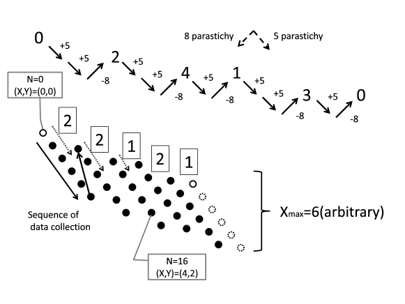
Figure 23: How to make an encircling layer of seeds on a parastichy lattice with a parastichy pair of $(Q,Q^{\prime})=(5,8)$. See Table 1 and the text.

The above method of data collection makes use of the 1-2 sequence. If one were interested not in numbering, but only in picking seeds to make a front circle, then it is sufficient to know a periodic 1-2 sequence. The periodic 1-2 sequence has period $Q$; all sequences 22121, 12122, 12212, 21221 and 21212 for $Q=5$ are regarded as equivalent. A periodic 1-2 sequence may be deduced recursively by simple rules to replace 2 with 21 and 1 with 2;

$$1 \rightarrow 2.$$

$$2 \rightarrow 21,$$ (83)

For the main sequence of phyllotaxis, starting from

$$Q=3:\quad 2\quad 2\quad 1,$$ (84)

one gets

$$5:\quad 21\quad 21\quad 2,$$

then

$$8:\quad 21\ 2\quad 21\ 2\quad 21,$$

and so on. The rules in (83) may remind Fibonacci’s original problem, in which 1 and 2 correspond to new and mature pair of rabbits. The 1-2 sequence in the correct order is obtained by reversing the sequence before applying (83). It goes as follows:

$$3:221$$

$$122$$

$$5:22121$$

$$12122$$

$$8:22122121$$

$$12122122$$

$$13:2212212122121$$

$$1212212122122$$

$$21:221221212212212122121$$

$$121221212212212122122$$

$$34:2212212122122121221212212212122121$$

The 1-2 sequence depends on $Q^{\prime}$ too. For instance, it is 21211 for $(Q,Q^{\prime})=(5,7)$, while 22121 for $(Q,Q^{\prime})=(5,8)$. Given a 1-2 sequence for a pair, 1-2 sequences for other pairs in the same Fibonacci sequence are routinely derived, according to the rule of reversal and replacement. From 21211 for $(Q,Q^{\prime})=(5,7)$, the rule gives 2221221 for the next pair $(Q,Q^{\prime})=(7,12)$ of the $(5,7)$ sequence, 5, 7, 12, 19, $\cdots$. The result is confirmed by the method of Table 1.

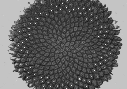
Figure 24: Digitizing an image from Jean (1994) by way of illustration. See the text for a procedure of making the encircling front layer. The direction of the fundamental spiral is opposite to that of Fig. 20.

Returning to the subject, let us take the cover image of Jean (1994) as an example. The first thing to do is to detect a shell layer of a well-defined encircling lattice spanned by opposed parastichies. In Fig. 24, there are $Q=34$ main parastichies involuting clockwise and $Q^{\prime}=55$ steeper opposite parastichies ($R=13$). The ordered 1-2 sequence for $Q=34$ is given just above. For simplicity, let us choose $X_{\rm max}=3$ for the thickness of the front layer. A procedure is: (i) import the image into the digitizer. (ii) Set a Cartesian coordinate system with proper scales of $x$ and $y$ axes. (iii) Fix the outermost layer of the primordia front according to the 1-2 sequence. Check if the front closes properly (the top and bottom of Fig. 23). (iv) Start clicking the seeds in sequence (the middle of Fig. 23). (v) Index the digitized Cartesian coordinates by (81) and (82).

The parastichy pair easiest to follow with the eye is to be used as $(Q,Q^{\prime})$, but the choice is not unique. The same index system is obtained if a lower parastichy pair is used, namely $(Q^{\prime}-Q,Q)$, $(2Q-Q^{\prime},Q^{\prime}-Q)$, etc.

Parastichy numbers of a multijugate system have a common divisor $J$, so that they are expressed as $J(Q,Q^{\prime})$ in terms of coprime integers $Q$ and $Q^{\prime}$. To close the primordia front of the $J$-jugate system, $Q$ steps of a 1-2 sequence are repeated $J$ times. Meanwhile, the $Y$ coordinate runs through $JQ$ integers from 0 to $JQ-1$. The plastochron index is given by (81). The jugacy index of the numbering system proposed in Sec. 2.2.2 shifts orderly along parastichies. For the seed at $(X,Y)$, it is given by

$${\rm Jugacy\ Index:}\quad j={\rm mod}(-PX+P^{\prime}Y,J)$$ (85)

by means of integers $P$ and $P^{\prime}$ satisfying $PQ^{\prime}-P^{\prime}Q=\pm 1$.

References

- Church (1904) Church, A. H., 1904. On the Relation of Phyllotaxis to Mechanical Laws. On the Relation of Phyllotaxis to Mechanical Laws. Williams & Norgate, London.
- Erickson (1983) Erickson, R. O., 1983. The geometry of phyllotaxis. In: Dale, J., Milthorpe, F. (Eds.), The Growth and functioning of leaves: proceedings of a symposium held prior to the thirteenth International Botanical Congress at the University of Sydney, 18-20 August 1981. Cambridge University Press, pp. 53–88.
- Fujita (1942) Fujita, T., 1942. Zur Kenntnis der Organstellungen im Pflanzenreich. Jpn. J. Bot. 12, 1–55.
- Green and Baxter (1987) Green, P. B., Baxter, D. R., 1987. Phyllotacticpatterns: Characterization by geometrical activity at the formative region. Journal of Theoretical Biology 128, 387–395.
- Hardy and Wright (1979) Hardy, G., Wright, E., 1979. An Introduction to the Theory of Numbers. Oxford Science Publications. Clarendon Press.
- Hotton (2003) Hotton, S., 2003. Finding the center of a phyllotactic pattern. Journal of Theoretical Biology 225 (1), 15 – 32.
- Hotton et al. (2006) Hotton, S., Johnson, V., Wilbarger, J., Zwieniecki, K., Atela, P., Golé, C., Dumais, J., 2006. The possible and the actual in phyllotaxis: Bridging the gap between empirical observations and iterative models. Journal of Plant Growth Regulation 25, 313–323.
- Jean (1983) Jean, R. V., 1983. Allometric relations in plant growth. Journal of Mathematical Biology 18, 189–200.
- Jean (1994) Jean, R. V., 1994. Phyllotaxis: A Systemic Study in Plant Morphogenesis. Cambridge Univ. Press, Cambridge, New York.
- Kiisk (2011) Kiisk, V., 2011. Digitizer. http://www.physic.ut.ee/ kiisk/files-eng.htm.
- Kumazawa and Kumazawa (1971) Kumazawa, M., Kumazawa, M., 1971. Periodic variations of the divergence angle, internode length and leaf shape, revealed by correlogram analysis. Phytomorphology 21, 376–389.
- Maksymowych and Erickson (1977) Maksymowych, R., Erickson, R. O., 1977. Phyllotactic change induced by gibberellic acid in xanthium shoot apices. American Journal of Botany 64, 33–44.
- Matkowski et al. (1998) Matkowski, A., Karwowski, R., Zagórska-Marek, B., 1998. Two algorithms of determining the middle point of the shoot apex by surrounding organ primordia positions and their usage for computer measurements of divergence angles. Acta Soc. Bot. Pol. 67, 151–159.
- Meicenheimer (1986) Meicenheimer, R. D., 1986. Role of parenchyma in Linum usitatissimum leaf trace patterns. American Journal of Botany 73, 1649–1664.
- Meicenheimer and Zagórska-Marek (1989) Meicenheimer, R. D., Zagórska-Marek, B., 1989. Consideration of the geometry of the phyllotaxic triangular unit and discontinuous phyllotactic transitions. Journal of Theoretical Biology 139, 359–368.
- Mirabet et al. (2012) Mirabet, V., Besnard, F., Vernoux, T., Boudaoud, A., 2012. Noise and robustness in phyllotaxis. PLoS Comput Biol 8, e1002389.
- Mitchell (2009) Mitchell, M., 2009. Engauge Digitizer - Digitizing software. http://digitizer.sourceforge.net/.
- Okabe (2011) Okabe, T., 2011. Physical phenomenology of phyllotaxis. Journal of Theoretical Biology 280, 63–75.
- Okabe (2012) Okabe, T., 2012. Vascular phyllotaxis transition and an evolutionary mechanism of phyllotaxis. http://arxiv.org/abs/1207.2838.
- Richards (1951) Richards, F. J., 1951. Phyllotaxis: Its quantitative expression and relation to growth in the apex. Philos. Trans. R. Soc. B 225, 509–564.
- Ridley (1982) Ridley, J. N., 1982. Packing efficiency in sunflower heads. Math. Biosci. 58, 129–139.
- Rivier et al. (1984) Rivier, N., Occelli, R., Pantaloni, J., Lissowski, A., 1984. Structure of Bénard convection cells, phyllotaxis and crystallography in cylindrical symmetry. J. Phys. (Paris) 45, 49–63.
- Rutishauser (1998) Rutishauser, R., 1998. Plastochrone ratio and leaf arc as parameters of a quantitative phyllotaxis analysis in vascular plants. In: Jean, R. V., Barabé, D. (Eds.), Symmetry in plants. World Scientific, pp. 171–212.
- Ryan et al. (1991) Ryan, G. W., Rouse, J., Bursill, L., 1991. Quantitative analysis of sunflower seed packing. Journal of Theoretical Biology 147 (3), 303–328.
- Sadoc et al. (2012) Sadoc, J.-F., Rivier, N., Charvolin, J., 2012. Phyllotaxis: a non-conventional crystalline solution to packing efficiency in situations with radial symmetry. Acta Crystallographica Section A 68 (4), 470–483.
- Swinton (2012) Swinton, J., 2012. The fundamental theorem of phyllotaxis revisited. http://arxiv.org/abs/1201.1641v2.
- Szymanowska-Pulka (1994) Szymanowska-Pulka, J., 1994. Phyllotactic patterns in capitula of Carlina acaulis L. Acta Soc. Bot. Pol., 229–245.
- van Iterson (1907) van Iterson, G., 1907. Mathematische und Mikroskopisch-Anatomische Studien über Blattstellungen. G. Fischer, Jena.
- Vogel (1979) Vogel, H., 1979. A better way to construct the sunflower head. Mathematical Biosciences 44 (3-4), 179–189.
- Williams (1974) Williams, R., 1974. The shoot apex and leaf growth: a study in quantitative biology. Cambridge University Press.
- Zagórska-Marek (1994) Zagórska-Marek, B., 1994. Phyllotaxic diversity in Magnolia flowers. Acta Societatis Botanicorum Poloniae 63, 117–137.