Revisiting Multi-Subject Random Effects in fMRI: Advocating Prevalence Estimation

Abstract

Random Effects analysis has been introduced into fMRI research in order to generalize findings from the study group to the whole population. Generalizing findings is obviously harder than detecting activation in the study group since in order to be significant, an activation has to be larger than the inter-subject variability. Indeed, detected regions are smaller when using random effect analysis versus fixed effects. The statistical assumptions behind the classic random effects model are that the effect in each location is normally distributed over subjects, and “activation” refers to a non-null mean effect. We argue this model is unrealistic compared to the true population variability, where, due to functional plasticity and registration anomalies, at each brain location some of the subjects are active and some are not. We propose a finite-Gaussian–mixture–random-effect. A model that amortizes between-subject spatial disagreement and quantifies it using the “prevalence” of activation at each location. This measure has several desirable properties: (a) It is more informative than the typical active/inactive paradigm. (b) In contrast to the hypothesis testing approach (thus t-maps) which are trivially rejected for large sample sizes, the larger the sample size, the more informative the prevalence statistic becomes.

In this work we present a formal definition and an estimation procedure of this prevalence. The end result of the proposed analysis is a map of the prevalence at locations with significant activation, highlighting activations regions that are common over many brains.

1 Introduction and Motivation

A typical cognitive fMRI study entails the group-wise localization of brain regions with evoked responses to a given cognitive stimulus. Individual statistical maps containing regression coefficients per voxel are combined across subjects to allow for group wise inference using “Random Effects Inference”. This inference has become standard since it offers reproducible findings (Friston et al. [10]). Its rationale is to compare the estimated effect to its variability over different replications with different subjects. A location is declared active if the observed effect is improbable, compared to the sampling variability, when assuming no activation.

The statistical assumptions behind the classic random effects approach are: (a) Homogeneity: at a fixed location, all subjects are either active or inactive. (b) Shift alternative: “activation” refers to a non-zero average effect over all subjects. (c) Gaussianity: the voxel-wise effect is Gaussian distributed over subjects.

Unfortunately, these assumptions rarely hold. For assumption (a) to be violated, it suffice for voxels to contain different structural and/or functional information across subjects, which is indeed the case; As put in Thirion et al. [22]: “spatial mis-registration implies that at a given voxel, i.e. a given position in MNI space, some subjects have activity while other subjects do not…”. Also in Fedorenko et al. [8]: “… activations land in similar but mostly non overlapping anatomical locations”. The visual motion area (MT) has been noted to vary over individuals by more than 2 cm after Talaraich normalization. The primary visual cortex has also been noted to vary in size– up to two fold over different subjects [19]. Assumption (b) is just a matter of convention: should locations where only 50% of subjects truly have non-zero activation should be called “active” or “inactive”? Finally, regarding (c), large deviations from the Gaussianity assumption have been demonstrated in several large studies (eg. Thirion et al. [22] and section 3 herein). This would typically affect sensitivity but not specificity, as the t-test is known to be conservative under symmetric but heavier-than–Gaussian tailed distribution [1]. In the following, we argue this is indeed the case of group fMRI studies.

Spatial smoothing of the signal is the typical solution for the above violations. It will spatially smear the signal so that between-subjects agreement is larger. It will also alleviate the Gaussianity assumption via the central limit theorem. Alas, spatial smoothing comes at the cost of spatial precision and does not address the inherent inappropriateness of the model.

In this work we take a different path; Without spatially smoothing the parametric maps, our model allows for voxels mapped to the same location to contain some proportion of both active and inactive individuals. The suggested model is both statistically realistic and explicitly allows for spatial disagreement over subjects– due to either brain plasticity or mis-registration. This amortizes the mis-registration effects while allowing to highlight regions of agreement over subjects with high spatial precision. We also argue that the proportion of the active sub population at each location (“prevalence”) is a more interesting parameter than the mean activation or the level of significance as appear in p-value maps. In particular when large samples are available and a significance test becomes non-informative, such as in Thyreau et al. [23]. In the following sections we try to formalize and justify the population-mixture assumption. Section 2 formalizes this intuition, which is applied to a large fMRI study in section 3. A discussion follows in section 4.

2 Method

2.1 Distribution of the Voxel-Wise Effects Over Subjects

We propose a voxel-wise adaptation of classical random-effect model. Recalling the random effect model:

$$y_{i}(t,v)=X_{i}(t)\beta_{i}\left(v\right)+\epsilon_{i}(t,v)$$ (2.1)

Where $y_{i}(t,v)$ is the fMRI signal of subject $i$ at time $t$ in voxel $v$. The expected (unscaled) signal induced by a stimulus is denoted by $X_{i}(t)$ and assumed known (see Worsley et al. [26] for details). Measurement error, intra-subject psychological variability and unmodeled effects are captured by $\epsilon_{i}\left(t,v\right)$. The subject specific effect induced by a stimulus in voxel $v$, is denoted by $\beta_{i}\left(v\right)$ . As previously mentioned, in the classical random effects model it is assumed to be Gaussian distributed over subjects, i.e. $\forall i=1,...,n:f(\beta_{i})=\phi_{\mu,\sigma^{2}_{\beta}}\left(\beta_{i}\right)$. For the reasons described in the introduction, we will now allow it to be a mixture of two populations: The “inactive” population centred at zero and the “active” population with a non-zero center. After omitting the voxel index $v$, the probability density function (PDF) of this mixture is given by:

$$f\left(\mbox{$\beta$}_{i}\right)=\left(1-p\right)f_{1}\left(\beta_{i}\right)+pf_{2}\left(\beta_{i}\right)$$ (2.2)

Where $f_{1}\left(.\right)$ is a symmetric distribution around zero, $0\leq p\leq 1$ and $f_{2}\left(.\right)=\phi_{\mu,\sigma^{2}}\left(.\right)$ with the mean effect $\mu$ allowed to be positive or negative like in the classical random effects setup.

2.2 Toy Example

To demonstrate that eq. 2.2 amortizes brain plasticity and mis-registration consider the following example: All subjects have a simple signal in their two dimensional “brains” as depicted in figure 2.1-A . The signal is similar across subjects, but not identical, in the sense that different subjects are allowed to have differently ellipse-shaped signals– mimicking functional plasticity. The centres are also changing slightly between subjects, mimicking misregistration effects. Figure 2.1-B depicts the relative frequency of the active subgroup overlap, over brains. We then introduce inter-subject variability for both the active and inactive subgroups and estimate $p$ using 100 “scans”. First, using our assumed variability model (2.1-C) and then using a mispecified model, to demonstrate robustness (2.1-D).

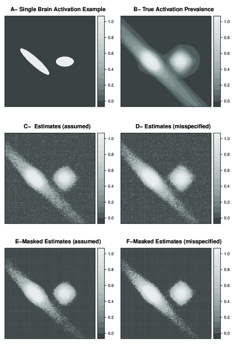
Figure 2.1: Toy Signal in Two Dimensional “Brain”. Figure A portrays the activation region in a single arbitrary “brain”. Figure B portrays the true prevalence (relative frequency) of the activation at each location after perturbing A to yield 100 “brains”, representing functional plasticity and misregistration. Figure C portrays the estimated prevalence from 100 scans with an effect variability obeying the assumptions of eq 2.3:
$(1-p)\cdot(0.88\mathcal{N}(0,0.15)+0.12\mathcal{N}(0,1))+p\cdot\mathcal{N}(1,0.25)$.
Figure D is similar to C. It demonstrates the prevalence estimator’s robustness to the mispecification of the active sub-population. The effect’s variability is given by:
$(1-p)\cdot(0.88\mathcal{N}(0,0.15)+0.12\mathcal{N}(0,1))+p\cdot(0.88\mathcal{N}(1,0.15)+0.12\mathcal{N}(1,1))$. Figures E and F are the same as C and D (respectively) after masking the insignificant prevalences using Wilcoxon’s signed rank statistic while controlling the FDR at 0.05

2.3 Estimation Using Self-Referential Task fMRI Data

In classical random-effects analysis, one would estimate the parameters of interest, by deriving the marginal distribution of $y_{i}(t,v)$ mixed by $f\left(\mbox{$\beta$}\right)$. In the fMRI literature it is more common to use a two-level approach: first estimate the subject effect, and then estimate the random effect parameters (Mumford and Nichols [14], Xu et al. [27]). These are known as the first and second level respectively. We adopt this approach for convenience, both mathematical and computational, but following a referee’s comment, we wish to note that proper estimation is still a matter of debate (e.g. Chen et al. [4]) and discuss the implications of the path we chose in C.

Due to the two-level approach, and since $\beta_{i}\left(v\right)$ are estimated and not observed directly, we have to allow for their measurement error. The second level effect distribution is given by 2.2 where $f_{1}\left(.\right)$ allows for first level variance. After considering various distributions for the inactive group– Gaussian, Cauchy, Laplace and Logistic– we have chosen a centred two-component–Gaussian-scale-mixture, which was also adopted in Woolrich [24]. Figure 2.2 demonstrates the three component Gaussian mixture typically fits the data better than other candidate distributions.

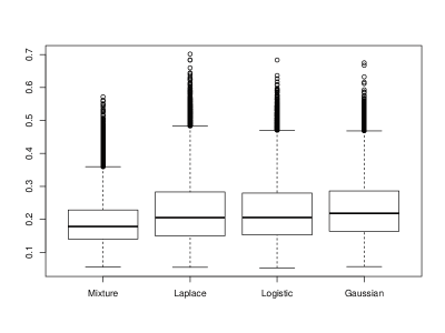
Figure 2.2: Distribution of Kolmogorov Smirnov test statistic over voxels, comparing different fitted distributions to data. To avoid over fitting, a train-test data split has been used. Boxplots are sorted by the median.

By redefining $f_{1}(.)=\frac{1}{1-p}\left(p_{1}\phi_{0,\sigma_{1}^{2}}+p_{2}\phi_{0,\sigma_{2}^{2}}\right)$, $p_{3}=p$, and keeping the standard $f_{2}\left(.\right)=\phi_{\mu,\sigma^{2}}\left(.\right)$ we get a three component mixture:

$$f(\beta_{i})=p_{1}\phi_{0,\sigma_{1}^{2}}(\beta_{i})+p_{2}\phi_{0,\sigma_{2}^{2}}(\beta_{i})+p_{3}\phi_{\mu,\sigma_{3}^{2}}(\beta_{i})$$ (2.3)

Where $p_{1,}p_{2,}p_{3}$ are the voxel-wise mixing proportions, naturally summing to 1, and $\phi_{mean,variance}$ are Gaussian PDFs allowed to have voxel-specific parameters.

We are now left with the problem of estimating the parameters of eq. 2.3: $\left(p_{1},p_{2},p_{3},\mu,\sigma_{1}^{2},\sigma_{2}^{2},\sigma_{3}^{2}\right)$. We use the expectation maximization algorithm (EM) to maximize the likelihood. We note that as in any mixture problem, identification problems arise. Even with the variances constrained so that $\sigma_{1}^{2}<\sigma_{2}^{2}$, any two-component–mixture can be parametrized as $\left(p_{1},p_{2},0,\bullet,\sigma_{1}^{2},\sigma_{2}^{2},\bullet\right)\cup\left(\bullet,p_{2},\bullet,0,\sigma_{1}^{2},\sigma_{2}^{2},\sigma_{1}^{2}\right)\cup\left(p_{1},\bullet,\bullet,0,\sigma_{1}^{2},\sigma_{2}^{2},\sigma_{2}^{2}\right)$ where $\bullet$ denotes a free parameter. We alleviate this problem by constraining the parameter space; In order to allow the interpretation of $p_{3}$ as the prevalence of activation, it is set to zero where the active sub-group is very similar to the inactive group. The threshing boundaries are an adaptation of the estimation limits in Donoho and Jin [7]. Particularly $p_{3}=0$ if the unconstrained prevalence estimate is smaller than $\exp\left[-\frac{\mu^{2}}{2(p_{1}\sigma_{1}^{2}+p_{2}\sigma_{2}^{2})}\right]$ This form has the following desired qualities: (a) Donoho and Jin [7], show (figure 1) that prevalence values violating this constraint are inestimable. (b) It forces $p_{3}\rightarrow 0$ as $\mu\rightarrow 0$ permitting $p_{3}$ to be interpreted as the activation prevalence. (c) The constraint is more restrictive as the variance of the null population increases.

Once the prevalence has been estimated, the next natural question is “could it be null?”. The testing stage is a separate problem we will discuss only briefly and for which many solutions might be considered. See Roche et al. [17] for some examples. Note however, that unlike the classical random-effect setup, this null is not tested against a shift alternative $(H_{1}:p_{3}=1;\mu\neq 0)$, but rather against a mixture alternative $(H_{1}:p_{3}>0;\mu\neq 0)$. This is because we consider as “active” any location with a non-null prevalence of activation. The generalized likelihood ratio test is not useful in this case due to mathematical and computational complexities (see Garel [12] or Delmas [6]). Instead, we use the Wilcoxon signed-rank statistic, and this for several reasons: (a) It is robust to model assumptions. (b) It is sensitive to location and shape shifts– both present when considering mixture alternatives. (c) It is easy to compute and interpret. (d) Surprisingly, it is more powerful than the group-t-test in our setup. We return to this point with real fMRI data in our hands in section 3.2.

3 Results

The proposed model was used to analyze fMRI data of 64 subjects performing a self-referential task making judgements about trait adjectives. See A for details. This is an unusually large study, offering the opportunity to validate the distributional assumptions presented. The data has not been spatially smoothed, except for some voxel blending due to the spatial normalization to the MNI template. We advocate the use of unsmoothed data to avoid the notorious spatial smearing of the signal (e.g. Saxe et al. [20]) which compromises spatial accuracy.

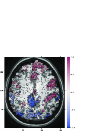
Figure 3.1: Estimated signed-prevalence: $\hat{p_{3}}\cdot sign{(\hat{\mu})}$. Masked at significant (prevalence>0) locations using the signed-rank test statistic with FDR control using B-H at FDR<0.1. Prevalence contour lines were added to help visualize the shape of the activation regions.

The SPM of the prevalence estimates is denoted $SPM\left\{p_{3}\right\}$ and demonstrated in figures 3.1 and 3.3-A. This estimate is compared to the standard second-level t-statistic depicted in 3.3-C. The boundaries of the activation region exhibit a smooth decay of $\hat{p}_{3}$ from $1$ to $0$ (more noticeable in 3.3-A). This phenomenon has already been observed by others, albeit with different interpretation: “Deviation from normality of the effects… coincides with the boundaries of activated areas” (Thirion et al. [22]). Since the phenomenon is to be expected given our motivation we find its empirical manifestation to be convincing evidence in favour of our model, where non-Gaussianity stems from sub-populations mixing (recall, no smoothing has been applied to the data). Also note that the change in prevalence happens at different rates across the image which excludes voxel blending as a cause for the smooth decay in prevalence. To further justify the mixture assumption, in figure 3.2 we examine the effect estimates at several select locations which indeed demonstrate the non Gaussian nature of the data. Figure 2.2 demonstrates the mixture’s better fit is not limited to just some select locations, but rather occurs (on average) over the whole brain volume. We are thus confident that our mixture model is more appropriate for the data we encounter than the single Gaussian underlying the usual random-effects analysis.

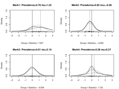
Figure 3.2: Distribution of Effect in Selected Locations: A density plot of the second-level effect distribution (solid grey line) along with the fitted mixture (solid black line) and its two weighted inactive components (dotted lines) and a third weighted active component (dash-dotted line). The mean of the active sub population is denoted with a vertical dashed line. Group t-statistic are included. The figures demonstrate the fit of the three component mixture to the second level effects at four locations referencing figure 3.3.

3.1 Interpreting SPM{prevalence}

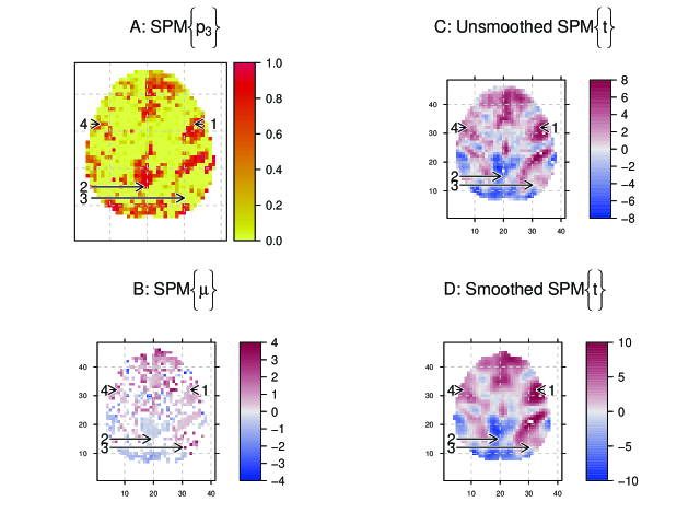
Figure 3.3: Maps of prevalence (A) and effects (B) compared with standard smoothed (D) and non-smoothed (C) second-level t-maps. The distribution of contrasts over individuals and value of t-statistic, in marked locations (1-4), can be seen in figure 3.2.

Figures 3.1 and 3.3 depict the estimated prevalence map. A higher prevalence means more people (in the population) show activation at that location. In particular, this says nothing about the magnitude of the activation (when present) quantified by $\mu$. High prevalence might be accompanied by high magnitudes of effect such as in mark 1 in fig. 3.2 and 3.3. This is the simplest pattern of “activation”. High prevalence might come with small effects (mark 2), which might be seen as statistical artifact which will probably be weeded out by testing, or as a prevalent small effects. The case of large signal with small prevalence (mark 3) might be seen as an effect, say, if it were at the boundary of an activation region, or an outlier, if it were spatially isolated. The t-statistic generally capture the existence of signal, but note that large variability around zero, might mask the existence of an active group such as in mark 4.

An example of these phenomena, can be seen in figure 3.3. In particular note the activation region near coordinates $x\approx\leavevmode\nobreak\ 20,y\approx\leavevmode\nobreak\ 40$ (or $x\approx 80,y\approx 150$ in fig. 3.1). This region is also apparent in the t-maps in figures 3.3 C and D , albeit it is less sharp due to what is probably a small subset of distinct (not to say “outliers”) subjects. Note the interesting lobe asymmetry of this region is completely masked in the standard smoothed $SPM\left\{t\right\}$ in figure 3.3- D.

Mark 2 in figure 3.2 also demonstrates that a negative effect, or contrast, is accommodated effortlessly. A negative “activated” population would mean a stimulus is negatively correlated with the BOLD signal, i.e., the neurons at that voxel are inhibited. If one were interested in positive (negative) effects alone, one could consider sign, or single-sided-hypothesis masking.

In summary, the prevalence estimate and the classical t-statistic are related, but capture different aspects of the activation pattern.

3.2 Group-T versus Group-Wilcoxon; Power Considerations

We have previously stated the Wilcoxon test should be preferred over the group-t-test for the localization problem. To see this last point we first note that more voxels have been found active; 11,817/27,401 using Wilcoxon versus 11,037/27,401 using the group-t-test. More importantly, the (Pitman) asymptotic relative efficiency of the two test statistics can be computed. We compute it using the average value of the nuisance parameters in the current study and find it to be $e_{Wilcox,T}=0.37$. That is, the Wilcoxon test is (asymptotically) about three times more efficient when testing for such mixture alternatives. This result is rather surprising. We elaborate on it in a separate methodological manuscript [18].

3.3 Spatial Accuracy and Stability

Visualizing the prevalence maps suggests they might display finer details than the t-maps. The boundaries of the common regions of activation, in figure 3.3-A, seem sharper than the t-map in 3.3-C (both unsmoothed). These details might be mere measurement noise, and thus come at the expense of stability. We would like to compare the spatial detail and stability of the two approaches quantitatively .

In order to compare the complexity of the emerging activation regions we computed the ratio between each region to its smallest enclosing cube. The more complicated the regions, the smaller is this ratio. We indeed find that the prevalence-defined-regions to be more complex. For instance, when half of the brain is “active” in the t-statistic sense, 117 out of the 286 active regions are singletons (one single voxel). This compares to 70 out of 247 such regions in the prevalence case. We also note that the median complexity of the t-regions, after excluding singletons, is 0.75 compared to a median of 0.5 for the prevalence regions.

To establish stability we compared the agreement in the activation regions defined by the two statistics, over two split samples. We find that using half of the data (n=32) the activation regions defined by the two statistics have essentially the same stability. For instance, when half of the brain is “active” the agreement of the t-regions over splits is 67% while the prevalence-regions’ agreement is 60%. We thus conclude that prevalence activation regions are indeed more complex and no-less stable.

4 Discussion

Much of the neuroscientific literature is devoted to the localization of brain activation. Little attention is given to the magnitude of the mean effect at active locations. This is no surprise given that the magnitude of the effect is variable even over different sessions for the same subject (Raemaekers et al. [16]). The suggested mixture-model approach admits a natural and intuitive quantification of the extent of activation at a location, not by its strength, but rather by its prevalence. The typical active/inactive qualification, is an instance of the suggested model, when $p=0$ or $p=1$. This estimation approach is particularly appropriate in large samples where prevalence estimators have low variance and significance tests are non informative and trivially rejected such as in Thyreau et al. [23]. While most appealing in large studies, the stability analysis in section 3.3 shows that the activation regions detected using the prevalence analysis are almost as stable as the group-t regions even with about 30 subjects. Moreover, they also enjoy finer spatial detail.

The concept of “prevalence” of activation is not a new one. In Friston et al. [9] the authors discuss how the use of conjunction hypotheses could allow to infer on the population without the explicit distributional assumptions in the random effect approach. The “number of subjects in a population showing the effect” denoted by $\gamma$ in their eq. (1), is precisely the prevalence discussed in this paper.

A test for “at least u out of n” active subjects was the approach taken in Heller et al. [13], which could possibly be seen as a testimator of this prevalence. Note though, that their partial conjunction inference measures the personal subject’s effect against the subject’s variability, while in the random effects approaches, including ours, the average effect is measured against the combined between-subject and within-subject variability. The estimate via partial conjunction may be therefore be 1 if all subjects’ effects are significant, yet the random effect prevalence be 0 if, say, half are on the positive and the other half are symmetrically negative. The opposite may true if individual variability is large the mean effect is small yet subjects’ effects are symmetrically distributed about this non-zero value. The prevalence defined in Heller et al. [13] is thus unrelated to our definition. For the typical definition of “activation”, it is the latter that should be preferred.

The use of finite mixtures in the context of fMRI has also been suggested. Xu et al. [27], motivated by the artifacts of spatial smoothing, recur to a finite Gaussian mixture to model variability between subjects. The number of components is however random and their weights depend on their proximity to an “activation center”. The spatial distribution of these activation centres is constructed as a multilevel point process. This construct allows to localize both a subject’s activation centres and the group activation centres. It also admits a concept of “prevalence” albeit somewhat more complicated than the one presented here.

The finite Gaussian mixture also appears in Woolrich [24]. In which the mixture is motivated by heavier-than-Gaussian tails of the effect distribution. The author uses a scale mixture to capture outliers in the effect distribution. The author does hint to the use of a “mean-shift model”, but again, only for the purpose of capturing outliers and not as a distinct sub population. In our work, we have indeed adopted the Gaussian scale mixture as the null population model, since we empirically found it to have a good fit.

5 Acknowledgements

We wish to thank Prof. Rafael Malach for introducing us to this problem.

The R implementation would not have been possible without the valuable work of Dr. Jonathan Clayden and the tractor.base package (Clayden et al. [5]).

Yoav Benjamini and Jonathan Rosenblatt were supported by a European Research Council Advanced Investigator Grant (P.S.A.R.P.S.).

Appendix A Data

We used data from 64 subjects (30 male, 34 female, mean age 30.3 +/- 6.5 SD years). These data were acquired at the University Medical Center Utrecht as part of a larger study (Zandbelt et al. [28], van Buuren et al. [3, 2]). All subjects were right-handed.

Subjects performed a self-referential task. In short, subjects had to make judgements about trait adjectives (for example ‘lazy’) in relation to themselves (Self condition), to someone else (Other condition), or they had to indicate whether this trait was socially desirable (Control condition). Conditions were presented in five separate blocks of eight trials (28s) each, alternated with rest periods of 30s. Total task duration was about 10min 32s fMRI measurements All imaging was performed on a Philips 3.0T Achieva whole-body MRI scanner. Functional were obtained using a 2D-EPI-SENSE sequence with the following parameters: voxel size 4 mm isotropic; TR= 1600 ms; TE = 23 ms; flip angle = 72.5°; matrix 52x30x64; field of view 208x120x256; 30-slice volume; SENSE-factor R=2.4 (anterior-posterior). A total of 395 functional images were acquired during the self-reflection task. After the acquisition of the functional images, an 3D Fast Field Echo (FFE) T1-weighted structural image of the whole brain was made (scan parameters: voxel size 1 mm isotropic, TR = 25 ms; TE = 2.4 ms; flip angle = 30°; field of view 256x150x204, 150 slices).

fMRI preprocessing and analysis Image preprocessing and analyses were carried out with SPM5 (http://www.fil.ion.ucl.ac.uk/spm/). After realignment, the structural scan was co-registered to the mean functional scan. Next, using unified segmentation the structural scan was segmented and normalization parameters were estimated. Subsequently, all scans were registered to a MNI T1-standard brain using these normalization parameters and a 3D Gaussian filter (8-mm full width at half maximum) was applied to all functional images. The preprocessed functional images were submitted to a general linear model (GLM) regression analysis. The design matrix contained factors modelling the onsets of the Self, Other and Control condition as well as the instructions that were presented during the task. These factors were convolved with a canonical hemodynamic response function [11]. To correct for head motion, the six realignment parameters were included in the design matrix as regressors of no interest. A high-pass filter was applied to the data with a cut-off frequency of 0.0055 Hz to correct for drifts in the signal. For the second-level analysis, we used the self condition versus baseline (rest) contrast.

Appendix B Statistical Method

As previously mentioned, estimation was performed by maximizing the likelihood using an EM algorithm. A major concern when solving several tens-of-thousands of EM problems, is speed, which is largely affected by the initialization values. Moment estimators are typical initialization values, but having six nonlinear moment equations these are hard to find. We thus employ a hybrid solution, in which we search over a grid of $\left(p_{1},p_{2}\right)$ values, solve the four moment equations given $\left(p_{1},p_{2}\right)$, and keep the highest likelihood value combinations as initialization values for the EM. This initialization heuristic allowed considerable speed gains during estimation.

Implementation was done in the R programming environment (R Core Team [15]). The described estimation procedure has been implemented in the R package FPF (fMRI Prevalence Finder) available from R-Forge (Theußl and Zeileis [21]) at http://rosenblatt1.r-forge.r-project.org/. See the package’s in-line help for details. The results in this paper were obtained using version 0.53 of the package. The raw data used is included in the package for reproducibility.

Appendix C Implications of two stage estimation

As presented in section 2, we use the first level effect estimates to fit a population distribution and estimate the prevalence. In particular, we do not use the first level variance estimates as done in some software suits ([see 25, footnote 1]). While chosen due to its simplicity, there are several considerations supporting our approach. First, there are the classical considerations: (a) the between-subject variance assumed to be of larger magnitude than the within-run variance and (b) the matter affecting only efficiency and not bias.

More importantly- the effect of inverse variance weighting is unclear, as we are no longer in the variance-components setup and we are no longer interested in the effect ($\mu$), but rather in the prevalence ($p$).

References

- Benjamini [1983] Benjamini, Y., 1983. Is the t test really conservative when the parent distribution is Long-Tailed? Journal of the American Statistical Association 78, 645–654.
- van Buuren et al. [2010] van Buuren, M., Gladwin, T., Zandbelt, B., Kahn, R., Vink, M., 2010. Reduced functional coupling in the defaultmode network during selfreferential processing. Human Brain Mapping 31, 1117–1127.
- van Buuren et al. [2011] van Buuren, M., Vink, M., Rapcencu, A., Kahn, R., 2011. Exaggerated brain activation during emotion processing in unaffected siblings of patients with schizophrenia. Biological Psychiatry 70, 81–87.
- Chen et al. [2011] Chen, G., Saad, Z., Nath, A., Beauchamp, M., Cox, R., 2011. FMRI group analysis combining effect estimates and their variances. NeuroImage .
- Clayden et al. [2011] Clayden, J., S.M.M., J.S., A., D.K., M., E.B., M., A.C., C., 2011. TractoR: Magnetic Resonance Imaging and Tractography with R. Journal of Statistical Software 44, 1–18.
- Delmas [2003] Delmas, C., 2003. On likelihood ratio tests in gaussian mixture models. Sankhya: The Indian Journal of Statistics (2003-2007) 65, pp. 513–531.
- Donoho and Jin [2004] Donoho, D., Jin, J., 2004. Higher criticism for detecting sparse heterogeneous mixtures. Annals of Statistics 32, 962–994. Cited By (since 1996) 88.
- Fedorenko et al. [2010] Fedorenko, E., Hsieh, P., Nieto-Castanon, A., Whitfield-Gabrieli, S., Kanwisher, N., 2010. New method for fMRI investigations of language: Defining ROIs functionally in individual subjects. Journal of Neurophysiology 104, 1177–1194.
- Friston et al. [1999] Friston, K., Holmes, A., Worsley, K., 1999. How many subjects constitute a study? NeuroImage 10, 1–5.
- Friston et al. [2002] Friston, K., Penny, W., Phillips, C., Kiebel, S., Hinton, G., Ashburner, J., 2002. Classical and bayesian inference in neuroimaging: Theory. NeuroImage 16, 465–483.
- Friston et al. [1994] Friston, K.J., Holmes, A.P., Worsley, K.J., Poline, J.P., Frith, C.D., Frackowiak, R.S.J., 1994. Statistical parametric maps in functional imaging: A general linear approach. Human Brain Mapping 2, 189–210.
- Garel [2007] Garel, B., 2007. Recent asymptotic results in testing for mixtures. Computational Statistics & Data Analysis 51, 5295–5304.
- Heller et al. [2007] Heller, R., Golland, Y., Malach, R., Benjamini, Y., 2007. Conjunction group analysis: An alternative to mixed/random effect analysis. NeuroImage 37, 1178–1185.
- Mumford and Nichols [2009] Mumford, J., Nichols, T., 2009. Simple group fMRI modeling and inference. NeuroImage 47, 1469–1475.
- R Core Team [2012] R Core Team, 2012. R: A Language and Environment for Statistical Computing. R Foundation for Statistical Computing. Vienna, Austria. ISBN 3-900051-07-0.
- Raemaekers et al. [2012] Raemaekers, M., du Plessis, S., Ramsey, N., Weusten, J., Vink, M., 2012. Test-retest variability underlying fMRI measurements. NeuroImage 60, 717–727. PMID: 22155027.
- Roche et al. [2007] Roche, A., Mariaux, S., Keller, M., Thirion, B., 2007. Mixed-effect statistics for group analysis in fmri: A nonparametric maximum likelihood approach. NeuroImage 38, 501 – 510.
- Rosenblatt and Benjamini [2013] Rosenblatt, J., Benjamini, Y., 2013. Another argument in favour of wilcoxon’s signed rank test. Submitted. Under review. .
- Sabuncu et al. [2009] Sabuncu, M., Singer, B., Conroy, B., Bryan, R., Ramadge, P., Haxby, J., 2009. Function-based intersubject alignment of human cortical anatomy. Cereb. Cortex , bhp085.
- Saxe et al. [2006] Saxe, R., Brett, M., Kanwisher, N., 2006. Divide and conquer: A defense of functional localizers. NeuroImage 30, 1088–1096.
- Theußl and Zeileis [2009] Theußl, S., Zeileis, A., 2009. Collaborative Software Development Using R-Forge. The R Journal 1, 9–14.
- Thirion et al. [2007] Thirion, B., Pinel, P., Mriaux, S., Roche, A., Dehaene, S., Poline, J., 2007. Analysis of a large fMRI cohort: Statistical and methodological issues for group analyses. NeuroImage 35, 105–120.
- Thyreau et al. [2012] Thyreau, B., Schwartz, Y., Thirion, B., Frouin, V., Loth, E., Vollstädt-Klein, S., Paus, T., Artiges, E., Conrod, P.J., Schumann, G., Whelan, R., Poline, J.B., 2012. Very large fMRI study using the IMAGEN database: sensitivity-specificity and population effect modeling in relation to the underlying anatomy. NeuroImage 61, 295–303.
- Woolrich [2008] Woolrich, M., 2008. Robust group analysis using outlier inference. NeuroImage 41, 286–301.
- Worsley et al. [2002] Worsley, K.J., Liao, C.H., Aston, J., Petre, V., Duncan, G.H., Morales, F., Evans, A.C., 2002. A general statistical analysis for fMRI data. NeuroImage 15, 1–15.
- Worsley et al. [1996] Worsley, K.J., Marrett, S., Neelin, P., Vandal, A., Friston, K., Evans, A., 1996. A unified statistical approach for determining significant signals in images of cerebral activation. Human Brain Mapping 4, 58–73.
- Xu et al. [2009] Xu, L., Johnson, T., Nichols, T., Nee, D., 2009. Modeling inter-subject variability in fmri activation location: A bayesian hierarchical spatial model. Biometrics 65, 1041–1051.
- Zandbelt et al. [2011] Zandbelt, B., van Buuren, M., Kahn, R., Vink, M., 2011. Reduced proactive inhibition in schizophrenia is related to corticostriatal dysfunction and poor working memory. Biological Psychiatry 70, 1151–1158.