Time-evolution of excitations in normal Fermi liquids

Abstract

We inspect the initial and the long time evolution of excitations a Fermi liquids by analyzing the time behavior of the electron spectral function. Focusing on the short-time limit we study the electron-boson model for the homogenous electron gas and apply the first order (in boson propagator) cumulant expansion of the electron Green’s function. In addition to a quadratic decay in time upon triggering the excitation, we identify non-analytic terms in the time expansion similar to those found in the Fermi edge singularity phenomenon. We also demonstrate that the exponential decay in time in the long-time limit is inconsistent with the GW approximation for the self-energy. The background for this is the Paley-Wiener theorem of complex analysis. To reconcile with the Fermi liquid behavior an inclusion of higher order diagrams (in the screened Coulomb interaction) is required.

I Introduction

Recently, short-time dynamics of excitations in a Fermi liquid has gained an increased attention due to the feasibility of new spectroscopic techniques  Krausz and Ivanov (2009); Cavalieri et al. (2007); Schultze et al. (2010); Ott et al. (2012) capable of accessing the attosecond time regime. For example in Cavalieri et al. (2007) a time delay in the range of 80 attoseconds between photoemission from the core-level of tungsten and from its conduction band has been measured. A further attosecond technique relies on the initial excitation of the system by an attosecond pulse and then tracing the excitation evolution by monitoring the response to a second phase-locked laser pulse Ott et al. (2012). This delivers a view on how quasiparticle states develop and decay in time on a scale well below the time that one may extract from their spectral width. The existent experiments on the attosecond time delay in photoemission call not only for a theoretical determination of the measured time delays but most importantly pose a question of what new physics can be gained from these highly sophisticated experiments. Does the spectral width of the QP peak encompass the complete information on how the QP is born/decays? As shown below, this is indeed not the case. The initial stage of the QP evolution follows a different time law as in the long time limit and the decay constants have a specific and materials dependent nature, endorsing thus the novel physics that can be gained with the attosecond metrology.

Theoretically, several methods can be used to explore the system’s dynamics numerically: the density matrix approach, the time-dependent density functional or density matrix renormalization group theories and the non-equilibrium Green’s functions Thygesen and Rubio (2007); Dahlen and van Leeuwen (2007); Thygesen and Rubio (2008); Pal et al. (2009, 2011); Uimonen et al. (2011). For the latter approach, which can be written in the form the Kadanoff-Baym equations, the two-times lesser (greater) Green’s functions $\mathbf{G}^{\lessgtr}(t_{1},t_{2})$ defined on the Keldysh time-loop contour are the central quantities. In the equilibrium situation these functions are directly related via the so-called Kubo-Martin-Schwinger boundary conditions to the advanced and retarded Green’s functions multiplied by the corresponding electron/hole distribution functions. In the nonequilibrium case they are complicated two-times quantities which can be found only approximately by using some approximations for the electron self-energy Kwong and Bonitz (2000); Ness et al. (2011). In order to judge the accuracy of such approximations it is desirable to have an analytic solution for some limiting cases.

On the basis of spectral moments calculations Vogt et al. (2004) for a 3D electron gas we conjectured an interpolative form of the electron spectral function at the energy $\epsilon$:

$$A(t;\epsilon)=A_{QP}(t;\epsilon)\,\exp\left(-\gamma(\epsilon)\frac{t^{2}}{t+\tau(\epsilon)}\right),$$ (1)

with $A_{QP}(t;\epsilon)$ the oscillatory quasiparticle part. At longer times $A(t;\epsilon)$ decays exponentially as expected from very general considerations based on the Landau theory of Fermi liquids and corrects a spurious divergence of the second spectral moment. The latter can be traced back to the fact that the exponential decay requires a certain time ($\tau(\epsilon)$) to set in and that initially the decay is quadratic:

$$\frac{d}{dt}A(t;\epsilon)\xrightarrow{t\rightarrow 0}-\sigma^{2}(\epsilon)\,t$$ (2)

The spectral function, being essentially the decisive equilibrium property, also enters the non-equilibrium two-times dynamics via the generalized Kadanoff-Baym Ansatz Lipavský et al. (1986); Kita (2010):

$$-i\mathbf{G}^{\lessgtr}(t_{1},t_{2})=\mathbf{G}^{r}(t_{1}-t_{2})\mathbf{G}^{\lessgtr}(t_{2})-\mathbf{G}^{\lessgtr}(t_{1})\mathbf{G}^{a}(t_{1}-t_{2}),$$ (3)

and, thus, can be used to calibrate the approximate numerical solutions. Although being quite natural, our underlying assumptions leading to (1) need to be rigorously verified, a task tackled here. In addition, it is desirable to quantify the parameters appearing in (1) in terms of measurable physical quantities and to offer a scheme for their computations. These are the goals of the present work.

The cumulant expansion is a well established procedure to study the dynamics of many-body systems in the time domain. It amounts to writing the electron Green’s function in the form:

$$\mathcal{G}(k,t)=\mathcal{G}^{0}(k,t)\,e^{C(k,t)},$$ (4)

The approach gained its wide recognition after Nozières and de Dominicis Nozières and De Dominicis (1969) demonstrated an exact solution of a complex integral equation for the cumulant function $C(k,t)$ for the Fermi edge singularity model. Initial applications to model systems include the Mahan’s treatment Mahan (1966) of the Fröhlich Hamiltonian, the Langreth’s study of the singularities in the X-ray spectra of metals Langreth (1970), or the fourth-order cumulant expansion for the Holstein model by Gunnarsson et al. Gunnarsson et al. (1994). More recently the approach was also applied, among others, to describe phenomena in realistic systems such as multiple plasmon satellites in Na and Al spectral functions Aryasetiawan et al. (1996) or in the valence photoemission of semiconductors Guzzo et al. (2011). Also similarity of this method to the coupled-cluster method broadly used in quantum chemistry is well known Schork and Fulde (1992).

Typically the method is applied to systems which allow a distinct separation of the Hamiltonian into the parts allowing for the analytical treatment and a coupling that needs to be treated perturbatively. A generic example is provided by the electron-boson Hamiltonian describing a fermionic subsystem (the usual quasiparticles) interacting with the bosonic excitations (e.g. phonon or the density fluctuations as will be considered below):

$$\mathcal{H}=\sum_{k}\epsilon_{k}c_{k}^{\dagger}c_{k}+\sum_{q}\omega_{q}b_{q}^{\dagger}b_{q}+\sum_{k,k^{\prime}}\sum_{q}\mathcal{V}^{q}_{kk^{\prime}}(b_{q}^{\dagger}+b_{q})c_{k}^{\dagger}c_{k^{\prime}},~{}$$ (5)

where we narrowed the domain of quantum numbers characterizing the system to a single wave-vector $\mathbf{k}$ as in the case of the homogeneous electron gas model. However, the formalism can easily be extended to realistic systems. Here $\omega_{q}$ describes the energies of bosonic excitations, $\epsilon_{k}=k^{2}/2$ is the usual particle dispersion in a weakly interacting Fermi liquid and $V^{q}_{k,k^{\prime}}$ is the coupling potential. We will use the concept of long-lived fermionic excitations (quasiparticles) as a defining property of the normal Fermi liquid state Giuliani and Vignale (2005). In fact this requirement is quite restrictive as it breaks down in, e.g., low-dimensional systems.

Under some circumstances the model (5) is exact: typically this is the case when certain matrix elements of the Coulomb interactions between a test particle (such as a deep core hole Langreth (1970) or a high-energy photoelectron Hedin et al. (1998)) are vanishingly small. For a more general scenario, e.g. as we consider here, the accurateness of (5) is less obvious Guzzo et al. (2011). In view of this fact it is interesting to consider the connections with other theories. Parallels between the cumulant expansion and the many-body perturbation theories (MBPT) in terms of the electron self-energy were explored by Aryasetiawan Aryasetiawan et al. (1996) in the lowest order. But does this correspondence hold at an arbitrary order? Development of the formalism and an answer to this question will be provided in Sec. II.

The cumulant function $C(k,t)$, we show, can be written very accurately in terms of the dynamical structure factor $\mathcal{S}(k,\omega)$. This allows us to obtain exact analytical results for the prefactor $\sigma^{2}(\epsilon)$ of the quadratic decay (2). It is interesting that also terms proportional to $(-it)^{3}$ can be written in a concise analytical form. These results do not require any further approximations in addition to the ones discussed in Sec. II and follow from exactly known sum-rules and the asymptotic behavior of $\mathcal{S}(k,\omega)$ (Sec. III).

The quasiparticle uncertainty $\sigma^{2}(\epsilon)$ (2) can alternatively be obtained from the zeroth spectral moment of the electron self-energy Pavlyukh et al. (2011). While this approach is perfectly justified for finite systems Pavlyukh and Berakdar (2011) a careful analysis must be done in the case of the homogenous electron gas (HEG) model. Here the difficulties arise from a particular asymptotic behavior of the electron self-energy: decay as $\omega^{-3/2}$ for $\omega\rightarrow\infty$ and its vanishing imaginary part for $\omega<\omega^{*}(k)$. In Sec. IV we trace the origins of these features. On the basis of the Paley-Wiener (PW) theorem Paley and Wiener (1934) we demonstrate that such restriction of the spectrum implies an unphysical spectral function which in the time domain asymptotically decays faster than the exponent. This is, however, a consequence of GW approximation for $\Sigma(k,\omega)$. The paradox is further resolved by considering higher order contributions to the electron self-energy.

II Cumulant vs. self-energy expansion

For the Hamiltonian (5) the interaction between fermionic and bosonic degrees of freedom is given by the fluctuation potential Hedin et al. (1998) with matrix elements:

$$\mathcal{V}^{q}_{k,k^{\prime}}=\frac{4\pi}{|\mathbf{k}-\mathbf{k}^{\prime}|^{2}}\,\rho^{q}_{\mathbf{k}-\mathbf{k}^{\prime}},$$ (6)

where $q$ is a quantum number characterizing the excited bosonic states and $\rho^{q}_{\mathbf{k}}$ is the $\mathbf{k}$th Fourier component of the fluctuation density operator between the ground state and a state with one boson with the quantum number $q$ excited. The choice of the interaction form is not arbitrary: it guarantees that the lowest order diagram for $\mathcal{G}(k,t)$ in the model (5) corresponds to the GW approximation (for more details on this approximation see Sec. IV) for the initial fermionic system.

It is instructive to derive $C(k,t)$ starting from MBPT and using the method of Aryasetiawan Aryasetiawan et al. (1996). By comparing the expansion of the exponential in (4) to that obtained by iterating the Dyson’s equation:

$$\mathcal{G}(k,t)=\mathcal{G}^{0}(k,t)\\ +\int\!\!d\tau\!\!\int\!\!d\tau^{\prime}\mathcal{G}^{0}(k,t-\tau)\,\Sigma(k,\tau-\tau^{\prime})\,\mathcal{G}(k,\tau^{\prime})$$ (7)

we can easily verify that $C(k,t)$ and $\Sigma(k,t)$ should have the same lowest order expression in terms of the interaction. We separately consider the particle ($k>k_{F}$) and the hole ($k<k_{F}$) cases. The non-interacting Green’s function is given by $\mathcal{G}_{+}^{0}(k,t)=-i\theta(t)\,e^{-i\epsilon_{k}t}$ and $\mathcal{G}_{-}^{0}(k,t)=i\theta(-t)\,e^{-i\epsilon_{k}t}$, respectively. We represent the full Green’s functions as $\mathcal{G}_{\pm}(k,t)=\mathcal{G}_{\pm}^{0}(k,t)\,e^{C_{\pm}(t)}$. These notations are different from the ones used by Langreth where they denoted two differently defined Green’s functions. For the electron self-energy we adopt the standard (non self-consistent) expression (cf. Eq. (25.1) of Hedin and Lundqvist (1970)):

$$\Sigma(k,t)=i\int\frac{d\mathbf{q}}{(2\pi)^{3}}\,\mathcal{W}(\mathbf{q}-\mathbf{k},t+\delta)\,\mathcal{G}^{0}(\mathbf{q},t),\quad\delta\rightarrow+0,$$

with the screened Coulomb interaction given by:

$$\mathcal{W}(k,\omega)=v(k)+v^{2}\Pi(k,\omega)=v(k)+\sum_{q}\frac{2\omega_{q}\big{|}\,V^{q}_{k}|^{2}}{\omega^{2}-\omega_{q}^{2}},$$ (8)

where $v(k)=4\pi/k^{2}$ is the Coulomb potential and $\Pi(k,\omega)$ is the full bosonic propagator or the density-density response function in this particular case. The latter is related by the fluctuation-dissipation theorem (cf. Eq. 3.74 of Giuliani and Vignale (2005)) to the dynamical structure factor:

$$\mathcal{S}(k,\omega)=-\frac{1}{\pi}\text{Im}\,\Pi(k,\omega).$$

For the $\omega$-dependent part of the screened Coulomb interaction we use the spectral representation:

$$\widetilde{\mathcal{W}}(\mathbf{k},t)=iv^{2}(k)\int_{0}^{\infty}\!\!d\omega\,\mathcal{S}(k,\omega)\,e^{-i\omega t},$$

where the dynamic structure factor is expressed in terms of the imaginary part of the dielectric function ($\varepsilon=\varepsilon^{\prime}+i\varepsilon^{\prime\prime}$):

$$\mathcal{S}(k,\omega)=\frac{k^{2}}{4\pi^{2}}\frac{\varepsilon^{\prime\prime}(k,\omega)}{|\varepsilon(k,\omega)|^{2}}\,\theta(\omega).$$

Clearly, four cases arise depending on the length of $\mathbf{q}$ and $\mathbf{k}$.

$k>k_{F}$ and $q>k_{F}$:

Inserting the expressions for $\Sigma$ and $\widetilde{\mathcal{W}}$ in Eq. (7) we obtain:

$$C_{+}(k,t)=-\int_{q>k_{F}}\!\frac{d\mathbf{q}}{(2\pi)^{3}}v^{2}(q)\int_{0}^{\infty}\!d\omega\,\mathcal{S}(\mathbf{q}-\mathbf{k},\omega)\,e^{-i\omega\delta}\\ \times\iint_{D_{+}}d(\tau\tau^{\prime})\,e^{i(\epsilon_{k}-\epsilon_{q}-\omega)(\tau-\tau^{\prime})},$$ (9)

where the integration domain is determined by the condition $\theta(t)\,\theta(t-\tau)\,\theta(\tau^{\prime})\,\theta(\tau-\tau^{\prime})$. This is, in fact, a finite domain which can be integrated as follows:

$$f(\nu)\equiv\iint_{D_{+}}d(\tau\tau^{\prime})\,e^{i\nu(\tau-\tau^{\prime})}=\int_{0}^{t}d\tau\int_{0}^{\tau}\!d\tau^{\prime}\,e^{i\nu(\tau-\tau^{\prime})}\\ =\int_{0}^{t}d\tau(t-\tau)\,e^{i\nu\tau}=\frac{1+i\nu t-e^{i\nu t}}{\nu^{2}}.$$ (10)

$k>k_{F}$ and $q<k_{F}$:

We have to use the hole propagator for the intermediate line. This changes the sign of the expression and modifies the integration domain which we represent as two terms:

$$\theta(t-\tau)\,\theta(\tau^{\prime})\,\theta(\tau^{\prime}-\tau)=\theta(t-\tau)\,\theta(\tau^{\prime})\,\big{(}1-\theta(\tau-\tau^{\prime})\big{)}$$ (11)

The first term here represents an additional contribution pertinent to GW approximation only:

$$\int_{-\infty}^{t}d\tau\int_{0}^{\infty}\!d\tau^{\prime}\,e^{i\nu(\tau-\tau^{\prime})}=-\frac{e^{i\nu t}}{\nu^{2}}.$$ (12)

For the second term in (11) we have the same form and sign as in (9). Thus, the integration over $q<k_{F}$ can be combined with (9) resulting in the sum over all momenta.

$k<k_{F}$ and $q<k_{F}$:

The procedure is similar with the only difference in the domain of the integration $D_{-}=\theta(-t)\,\theta(\tau-t)\,\theta(-\tau^{\prime})\,\theta(\tau^{\prime}-\tau)$ which also integrates in terms of $f(\nu)$:

$$\iint_{D_{-}}d(\tau\tau^{\prime})\,e^{i\nu(\tau-\tau^{\prime})}=\int_{t}^{0}d\tau\int_{\tau}^{0}\!d\tau^{\prime}\,e^{i\nu(\tau-\tau^{\prime})}=f(\nu).$$

Hence, $C_{-}(t)$ can be written in the same form as (9) and we will use $C(k,t)$ as a common symbol for both $C_{\pm}(k,t)$. There also is a contribution from the intermediate hole line $q>k_{F}$ to $C_{-}(t)$ which can be evaluated along the same lines as (12). Finally, we redefine the variable for momentum integration as $\mathbf{q}-\mathbf{k}\rightarrow\mathbf{q}$ and obtain in line with Langreth Langreth (1970):

$$C(k,t)=-\sum_{q}v^{2}(q)\int_{0}^{\infty}\!d\omega\,\,\mathcal{S}(q,\omega)\\ \times f\big{(}\epsilon_{|\mathbf{k}|}-\epsilon_{|\mathbf{k}+\mathbf{q}|}-\omega,t\big{)}.$$ (13)

The central quantity of this study – the dynamical structure factor – although expressed almost identically (except for the (12) terms) in the many-body perturbation and in the cumulant expansion theories, originates from different approximations. In the former case it is the vertex function in the expression for the self-energy that is neglected, while for the latter it is assumed that the Hamiltonian can be written in the electron-boson form (5). For the homogenous electron gas model the justification mostly comes from MBPT although $\mathcal{S}(k,\omega)$ can be rather complicated function even for simple systems Takada and Yasuhara (2002).

III Short and long time limits

Equation (13) is general enough to treat all the cases presented in Tab. 1. Compared to Eq. (44) of Langreth (1970) we additionally allow the test particle to scatter (i.e. to exchange its momentum with the bosonic excitations) whereas a deep core in Langreth (1970) is assumed to have an infinite effective mass. The short-time limit of the electron Green’s function crucially depends on the exact form of fermionic dispersion, on the boundness of the bosonic spectrum and on the actual form of the coupling potential.

Table 1: Electron-boson models and main results for the long and short-time limits of the electron Green’s function

Fermionic dispersion	Dispersionless phonons	Dispersionless plasmons	Electron-hole pairs
Deep hole: $H_{0}=Ec^{\dagger}c$		$\displaystyle C(t)\sim e^{-i\omega_{p}t}$ Langreth (1970)	$\displaystyle C(t)\sim-\alpha\big{[}\ln|Dt|\mp i\pi/2\,\mathrm{sgn}{t}\big{]}$ Langreth (1970)
Valence states: $\displaystyle H_{0}=\epsilon_{k}c_{k}^{\dagger}c_{k}$	$\displaystyle C(t)\sim\frac{1}{\omega_{0}}(2it)^{1/2}\,e^{-i\omega_{0}t}$ Mahan (1961)	$\displaystyle C(t)\sim e^{-i\omega_{p}t}$ Aryasetiawan (1996)	this work

As a first application we compute the leading expansion coefficients of the cumulant function in the short-time limit:

$$C(k,t)=-\frac{\sigma^{2}(k)}{2!}t^{2}+\frac{c_{3}(k)}{3!}t^{3}+\ldots$$ (14)

We note, however, that such expansion does not imply analyticity of the function in vicinity of $t=0$. Just the opposite, higher expansion coefficients diverge starting from $c_{6}$ in 2d case and from $c_{7}$ in 3d based on very general properties of the density-density response function ($\text{Im}\,\Pi(k,\omega)\sim\omega^{-4-d/2}$, p. 139 of Giuliani and Vignale (2005)). Although where the divergence occurs exactly can be modified by including higher order terms (in $\mathcal{S}(k,\omega)$) in the expression for the cumulant function, this will not restore the analyticity. The prefactor of the quadratic decay (Eq. (2)) can be computed by evaluating the second derivative of (13) at $t=0$:

$$\sigma^{2}=n\sum_{q}v^{2}(q)\,\mathcal{S}(q),$$ (15)

where the static structure factor is defined as

$$\mathcal{S}(q)=\frac{1}{n}\int_{0}^{\infty}\!\!d\omega\,\mathcal{S}(q,w)\xrightarrow{q\rightarrow 0}\frac{q^{2}}{2\omega_{p}(q)}.$$ (16)

It follows then that $\sigma^{2}$ is independent of $k$ and coincides with the local contribution to the zeroth spectral moment of the electron self-energy obtained by Vogt et al. Vogt et al. (2004). The long wave-length expression in Eq. (16) follows from the exactness of the random phase approximation (RPA) in this limit. In the opposite case (i.e. $q\rightarrow\infty$) the structure factor approaches unity, however, the subleading term RPA fails to reproduce. In order to accurately compute $\sigma^{2}$ the parameterized structure factor of Gori-Giorgi et al. Gori-Giorgi et al. (2000) based on the quantum Monte Carlo results was used Vogt et al. (2004). The convergence of the integral (15) is ensured by the limit:

$$\lim_{q\rightarrow\infty}q^{z+1}\big{[}\mathcal{S}(q)-1\big{]}=-\pi 2^{z}ng(0),$$ (17)

where $g(0)$ is the value of the pair correlation function for two electron at the same position and $z$ is the dimensionality of a system.

It is not obvious from the outset that the $c_{3}(k)$ coefficient should take a finite value: this heavily relies on the exact form of the structure factor in the asymptotic ($q\rightarrow\infty$) limit. By using the $f$-sum rule:

$$\int_{0}^{\infty}\!d\omega\,\omega\,\mathcal{S}(q,\omega)=n\epsilon_{q},$$ (18)

where $n$ is the electron density we obtain:

$$c_{3}(k)=-in\sum_{q}v^{2}(q)\Big{[}\big{(}\epsilon_{|\mathbf{k}|}-\epsilon_{|\mathbf{k}+\mathbf{q}|}\big{)}\,\mathcal{S}(q)+\epsilon_{q}\Big{]}.$$ (19)

In the simplest case of a hole state at the band’s bottom the convergence of the integral regardless of the system’s dimension ($z$) is guaranteed by the limit (17). For $k>0$ the term linear in $k$ vanishes after the angular integration and we finally obtain the $k$-independent result:

$$c_{3}=in\sum_{q}v^{2}(q)\,\epsilon_{q}\,\Big{[}\mathcal{S}(q)-1\Big{]}.$$

Finally we notice that the leading terms of Eq. (13) in the long time-limit are the constant and the linear ones, i.e., $C(k,t)\xrightarrow{t\rightarrow\infty}\gamma-i\,\Sigma(k,\epsilon_{k})t$ as expected from the exponential quasiparticle decay (cf. Eq. (7) of Aryasetiawan et al. (1996)).

Non-analyticity of the spectral function at $t=0$

The asymptotic behavior of the density-density response function at large $\omega$ leads to diverging expansion coefficients in Eq. (14). This, in turn, gives us a hint that the cumulant function is probably nonholomorphic at $t=0$. Such property is, however, not an exception, but rather the rule as Tab. 1 demonstrates. We will sketch below how all the results presented in this table can be obtained in a unified way from Eq. (13) and will also show that the same applies to the normal Fermi liquids, in particular due to the scattering of valence electrons with the generation of electron-hole pairs (viz. “this work” in Tab.  1).

One of the most interesting scenarios is the case of a core hole coupled to electron-hole excitations. In the limit of infinite mass of the fermion and $t\rightarrow\infty$ there is a singular term that arises from the frequency integration in Eq. (13):

$$C(t)=-\sum_{q}\frac{v^{2}(q)}{|\varepsilon(q,0)|^{2}}\int_{0}^{\infty}\!d\omega\,\frac{\omega}{q}\frac{1-e^{-i\omega t}}{\omega^{2}}\sim-\eta\big{[}\ln|Dt|+\frac{i\pi}{2}\,\mathrm{sgn}t\big{]}$$

where $0<\eta<\frac{1}{2}$ is called the Anderson singularity index Anderson (1967) which can be given in terms of the scattering phase shifts $\delta_{l}$ of the statically screened potential ($\mathcal{W}(q,0)$) as

$$\eta=2\sum_{l}(2l+1)\left(\frac{\delta_{l}}{\pi}\right)^{2}.$$

In the frequency domain the resulting spectral function exhibits a singularity $\frac{2\pi}{\Gamma(\eta)}\frac{\theta(-\omega)}{\omega^{1-\eta}}$ which for the finite hole’s mass and $z>1$ is completely washed out by the effect of scatterer recoil as was demonstrated by Nozières Nozières (1994). This equivalently can be seen from our model (13) where the momentum angular integration of the function $f\big{(}\epsilon_{|\mathbf{k}|}-\epsilon_{|\mathbf{k}+\mathbf{q}|}-\omega,t\big{)}$ removes the singularity.

The cumulant function resulting from the interaction with plasmons has a simple structure which likewise follows from (13) by using the limiting form of the structure factor:

$$\mathcal{S}(q,\omega)\xrightarrow{q\rightarrow 0}\frac{q^{2}}{8\pi}\frac{\omega_{p}(0)^{2}}{\omega_{p}(q)}\delta(\omega-\omega_{p}(q)).$$

In the frequency domain this leads to the main quasiparticle peak accompanied by a sequence of satellites displaced by $n\omega_{p}(0)$ Minnhagen (1975); Ness et al. (2011). In many realistic materials these are indeed observed features Aryasetiawan et al. (1996); Guzzo et al. (2011). Recalling our remark in the introduction concerning the current status of the experimental attosecond spectroscopy, it is obvious that these structures are interesting candidates for the tracking of the development of main and satellite peaks to their static limit.

Another interesting case, likewise in the $t\rightarrow\infty$ limit, arises from the polar coupling $\sim 1/q$ between an electron and the non-dispersive optical phonon with the energy $\omega_{0}$ Mahan (1966). It results in the effective structure factor $\mathcal{S}(q,\omega)\sim 1/q^{2}\delta(\omega-\omega_{0})$. There, the non-analytic terms stem from the momentum integration:

$$\sum_{q}\frac{1}{q^{2}}e^{-i\epsilon_{q}\tau}=\frac{4\pi}{(2\pi)^{3}}\int_{0}^{\infty}\!dq\,e^{-i\epsilon_{q}\tau}=\frac{1}{(2\pi)^{3/2}}\left(\frac{2}{i\tau}\right)^{1/2}.$$

For the momentum state $k=0$ we can use the representation of $f\big{(}\epsilon_{|\mathbf{k}|}-\epsilon_{|\mathbf{k}+\mathbf{q}|}-\omega,t\big{)}$ in terms of a single time-integral (10) and obtain:

$$C(0,t)\sim\int_{0}^{t}d\tau(t-\tau)\,\left(\frac{2}{i\tau}\right)^{1/2}e^{-i\omega_{0}\tau}\sim\frac{1}{\omega_{0}}(2it)^{1/2}\,e^{-i\omega_{0}t}.$$

In the opposite case, i. e. $t\rightarrow 0$, the non-analytic terms originate from the coupling to the particle-hole ($p\mathchar 45\relax h$) continuum. We can split the momentum integration into a finite interval $q<q_{c}$ yielding just the well-behaved analytic part of $C(k,t)$ and the interval extending to infinity. The value of $q_{c}$ can always be chosen large enough so that the real part of the dielectric function on the second interval approaches unity. This considerably simplifies the dynamical structure factor which results now from the imaginary part of the Lindhard formula (Eq. (5.35) of Hedin and Lundqvist (1970) for $z=3$) only:

$$S(q,\omega)=\frac{1}{\pi}\frac{1}{v(q)}\frac{\alpha r_{s}}{\tilde{q}^{3}}\left(1-\frac{1}{4}\left(\tilde{q}-\frac{\tilde{\omega}}{\tilde{q}}\right)^{2}\right),$$

where the tilde denotes the use of rescaled quantities, i.e. $q=\tilde{q}k_{F}$, $\omega=\tilde{\omega}\epsilon_{F}$, $\tilde{\tau}=\tau/\epsilon_{F}$ and so on. After the substitution $\tilde{\omega}=\tilde{q}^{2}+2\tilde{q}\lambda$ we can first integrate over the interval $|\lambda|<1$. This yields a trigonometric expression which is just a constant in the lowest order of $2\tilde{q}\tilde{\tau}$:

$$\int d\omega\,\mathcal{S}(q,\omega)\,e^{-i(\tilde{\omega}-\tilde{q}^{2})\tilde{\tau}}=\frac{1}{3\pi^{2}}k_{F}^{3}+\mathcal{O}(2\tilde{q}\tilde{\tau}).$$

The leading non-analytic term of the remaining momentum integral reads:

$$\frac{1}{(2\pi)^{3}}\int\!q^{2}dq\,v^{2}(q)\,e^{-2i\tilde{q}^{2}\tilde{\tau}}\sim-\frac{2}{k_{F}}\left(\frac{2i\tilde{\tau}}{\pi}\right)^{1/2}.$$

Finally we perform the time integration as in (10):

$$C(0,t)=\frac{2k_{F}^{2}}{3\pi^{2}}\int_{0}^{t}\!d\tau\,(t-\tau)\left(\frac{2i\tilde{\tau}}{\pi}\right)^{1/2}=-\frac{8}{45}(\alpha r_{s})^{2}\left(\frac{2it}{\pi}\right)^{5/2}.$$ (20)

Such time-dependence is easy to reconcile with well known asymptotic behavior of the electron self-energy as a function of frequency Bose and Fitchek (1975); Vogt et al. (2004):

$$\text{Im}\,\tilde{\Sigma}(k,\tilde{\omega})\xrightarrow{\omega\rightarrow\infty}=-\frac{16\sqrt{2}}{3\pi}\frac{(\alpha r_{s})^{2}}{\tilde{\omega}^{3/2}}.$$

To see the connection we express asymptotically the spectral function as $A(k,\omega)\sim C/\omega^{2+3/2}$ and perform the Fourier transform. Since at $\omega\rightarrow-\infty$ the spectral function decays faster, in fact on the GW level it is even zero below a certain threshold value of $\omega$, it is sufficient to perform the transform on a semi-bounded interval:

$$A(k,t)\sim\int_{\omega_{c}}^{\infty}\frac{d\omega}{2\pi}\frac{C}{\omega^{7/2}}\,e^{-i\omega t}.$$

Among several resulting terms one has to pick up the one independent of the cut-off $\omega_{c}$. It exhibits the same time-dependence and the density scaling $\sim(\alpha r_{s})^{2}$ as Eq. (20).

IV Self-energy in frequency space

In 1965 Lars Hedin formulated a system of functional equations Hedin (1965), carrying by now his name, that relate the electron self-energy $\Sigma(12)$, the irreducible polarization propagator $\mathcal{P}(12)$, the screened Coulomb interaction $\mathcal{W}(12)$, the vertex function $\Gamma(12;3)$ and the electron Green’s function $\mathcal{G}(12)$. The Hedin equations are becoming one of the major theoretical tools for the treatment of correlated many-particle systems Onida et al. (2002); Aryasetiawan and Miyake (2009); Ren et al. (2012). The homogeneous electron gas (HEG) in two or three dimensions is a prototypic model which allows for testing various approximations to the exact Hedin’s equations. Earlier applications revealed important features of the single-particle spectrum Lundqvist (1967, 1967, 1968). These single-shot calculations were extended by several authors to the self-consistent level von Barth and Holm (1996); Holm and von Barth (1998), higher order diagrams were included Shirley (1996); Takada (2001).

In view of large efforts devoted to the study of these model systems it is surprising that some aspects remained unnoticed. Thus, it is commonly believed that HEG in two or three dimensions serves as a perfect illustration of the Fermi liquid concept Giuliani and Vignale (2005), that is a many-body fermionic systems with long-lived excitations: quasiparticles. Two marked properties distinguish them from other excited states: i) they can be brought in a direct correspondence with real particles (electrons) of a fictitious non-interacting many-body system; ii) they are characterized by the life-time, which tends to infinity as the particle’s energy approaches the Fermi level ($\epsilon_{F}$). It also implies that asymptotically the decay is exponential $\exp(-\gamma t)$, with the decay constant being quadratically dependent on the energy ($\gamma(\epsilon)\sim\epsilon^{2}/\epsilon_{F}$). At $\epsilon\rightarrow\epsilon_{F}$ this constant can be computed perturbatively, and it is sufficient to consider the lowest-order term giving a non-vanishing imaginary part of the self-energy. In view of this it is intriguing that a rigorous proof can be given that the lowest-order diagram yield the spectral function inconsistent with the asymptotic exponential decay.

One recognizes that pronounced features in the spectral function appear at energies $E_{k}$ that are approximately given by $E_{k}=\epsilon_{k}+\Sigma(k,E_{k})$, where $\text{Im}\,\Sigma(k,\omega)\sim\delta(\omega-\epsilon_{\mathbf{|k+q|}}\pm\omega_{q})$. These resonances are surrounded by the incoherent background which has the same extend as the self-energy:

$$A(k,\omega)=\frac{1}{\pi}|\text{Im}\,\mathcal{G}(k,\omega)|\\ =\frac{1}{\pi}\frac{|\text{Im}\,\Sigma(k,\omega)|}{|\omega-\epsilon_{k}-\text{Re}\,\Sigma(k,\omega)|^{2}+|\text{Im}\,\Sigma(k,\omega)|^{2}}.$$ (21)

In the lowest order of the screened interaction a particle can only loose its energy ($\epsilon_{k}$) by generating a single bosonic excitation $\omega_{q}$. Since only a finite momentum can be transfered also $\omega_{q}$ is finite and, thus, the self-energy has a semi-bounded support (limited from below) (Fig. 1). From this, in view of (21) follows $A(k,\omega)=0$ for $\omega<\omega^{*}(k)$.

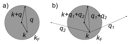
Figure 1: a) First and b) second order hole scattering mechanisms. While the two excitations in b) carry in total the same momentum as a single excitation in a) the energy transfer is much larger.

The last property allows us to apply the Paley-Wiener (PW) theorem Paley and Wiener (1934) which we present below for completeness in the original formulation:

Theorem 1

Let $\phi(x)$ be a real non-negative function not equivalent to zero, defined for $-\infty<x<\infty$, and of integrable square in this range. A necessary and sufficient condition that there should exist a real- or complex-valued function $F(x$) defined in the same range, vanishing for $x\geq x_{0}$ for some number $x_{0}$, and such that the Fourier transform $G(x)$ of $F(x)$ should satisfy $|G(x)|=\phi(x)$, is that

$$\int_{-\infty}^{\infty}\frac{|\log\,\phi(x)|}{1+x^{2}}\,dx<\infty.$$ (22)

The modern formulation  only slightly relaxes the conditions on the functions:

Theorem 2

For $\phi(x)\in L^{2}(\mathbb{R})$ and $\phi(x)>0$ the integral (22) converges $\iff$ there is a function $F\in L^{2}(\mathbb{R})$ with a semi-bounded support such that $\phi=|\mathcal{F}[F]|$ a. e. in $\mathbb{R}$, and $\mathcal{F}$ is the Fourier-Plancherel operator.

From here follows:

Corollary 1

$$F(y)=0\quad\text{for}\quad y<y_{0}\Rightarrow\int_{\mathbb{R}}\frac{|\log\,\phi(x)|}{1+x^{2}}\,dx<\infty\quad\Rightarrow\\ |\phi(x)|\xrightarrow{x\rightarrow\infty}\exp(-Bx^{\alpha}),\quad\text{where}\quad\alpha<1.$$

If we identify now $F$ with $A(k,\omega)$ the deviation from the exponential decay for $A(k,t)$ follows: a result in a clear contradiction with the Fermi liquid theory. Before proceeding with the resolution of the paradox we present our method for numerical calculation of $\omega^{*}(k)$. It is sufficiently general in the sense that there is no limitation on the dimensionality ($z$) of the system and it is not limited to the first order expression. From now on we will only be using rescaled quantitates, tilde will be omitted for clarity. In order to make the model amenable for the numerics we introduce the following representation of the screened Coulomb interaction:

$$\mathcal{W}^{0}(k,\omega)=\frac{v(k)}{2}\!\int\!d\lambda\,\left[\frac{w(k,\lambda)}{\omega-\Omega(k,\lambda)+i\eta}-\frac{w(k,\lambda)}{\omega+\Omega(k,\lambda)-i\eta}\right],$$ (23)

where $w(k,\lambda)$, $\Omega(k,\lambda)$ are some real functions that will be specified below. Our representation takes advantage of the fact that the imaginary part of the dielectric function and the screened Coulomb interaction is different from zero only in the stripe area in the $\omega\mathchar 45\relax k$ plane and along the plasmonic line Giuliani and Vignale (2005). The limits for the particle-hole continuum are given (for $z\geq 2$) by:

$$\max\Big{\{}0,\omega_{-}(k)\Big{\}}\leq|\omega|\leq\omega_{+}(k),\,\text{with}\quad\omega_{\pm}(k)=k^{2}\pm 2k,$$ (24)

where it is convenient to parameterize the trajectories on the stripe (24) as:

$$\Omega(k,\lambda)=k^{2}+2\lambda k.$$

Thus Eq. (23) is nothing but the spectral representation (see e. g. Eq. 4 of von Barth and Holm (1996)):

$$\mathcal{W}(k,\omega)=v(k)+\int_{0}^{\infty}\frac{2\omega^{\prime}B(k,\omega^{\prime})}{\omega^{2}-\omega^{\prime 2}}d\omega^{\prime},$$

The integral over $\lambda$ is to be understood in a generalized sense: this parameter can assume both discrete values when we describe a single excitation such as plasmon or be a continuous variable for particle-hole excitations. In the former case it reduces to the plasmon model approximation (cf. Eq. 25.11 of Hedin and Lundqvist (1970)):

$$\mathcal{W}^{0}(k,\omega)=v(k)\left[1+\frac{\omega_{p}^{2}(0)}{\omega^{2}-\omega_{p}^{2}(k)}\right].$$

The bare Coulomb part can also be obtained from (23): consider the limit $\Omega(k,\lambda)\rightarrow w(k,\lambda)\rightarrow\infty$. The fact that we can represent all contributions to $W(k,\omega)$ in a unified way is crucial for our discussion: one does not need to separately consider diagrams with bare or renormalized interaction lines. The former can be obtained from the general case by formally taking the limit of the final expression.

We write the Green’s function as:

$$\mathcal{G}^{0}(k,\omega)=\frac{n_{k}}{\omega-\epsilon_{k}-i\eta}+\frac{1-n_{k}}{\omega-\epsilon_{k}+i\eta},$$

where $n_{k}$ denotes the occupation of the state with the momentum $k$ and consider the two lowest order diagrams for the electron self-energy $\Sigma[\mathcal{G}^{0},\mathcal{W}^{0}]$:

$$\Sigma^{(1)}(1,2) = i\,\mathcal{G}^{0}(1,2)\,\mathcal{W}^{0}(1^{+},2),$$ (25a)

$$\Sigma^{(2)}(1,2) = i^{2}\!\iint\mathcal{W}^{0}(1^{+},4)\,\mathcal{G}^{0}(1,3)\,\mathcal{G}^{0}(3,4)$$ (25b)

$$\quad\quad\quad\quad\times\,\mathcal{G}^{0}(4,2)\,\mathcal{W}^{0}(3^{+},2)\,d(34).$$

Our representation of the screened Coulomb interaction allows to compute the electronic self-energy relatively easy using the maple computer algebra system . The final results can be recasted in the form of momentum and $\lambda$ integrals over complicated domains that we denote as $\mathcal{D}_{\pm}^{(i)}$, where $\pm$ designates particle (hole) state, and $(i)$ is the order of a diagram. Since we are only interested in the phase-space where each diagram contributes we skip here the explicit expressions for $\Sigma(k,\omega)$ and present only the results for $\mathcal{D}_{\pm}^{(i)}(k,\omega)$:

$$\mathcal{D}_{-}^{(1)} = n_{p}\,\delta\big{(}\omega-\epsilon_{p}+\Omega(q,\lambda)\big{)},$$ (26a)

$$\mathcal{D}_{-}^{(2a)} = (1-n_{p_{0}})\,n_{p_{1}}n_{p_{2}}\delta\big{(}\omega+\epsilon_{p_{0}}-\epsilon_{p_{1}}-\epsilon_{p_{2}}\big{)},$$ (26b)

$$\mathcal{D}_{-}^{(2b)} = n_{p_{0}}\delta\big{(}\omega-\epsilon_{p_{0}}+\Omega(q_{1},\lambda_{1})+\Omega(q_{2},\lambda_{2})\big{)},$$ (26c)

$$\mathcal{D}_{-}^{(2c)} = n_{p_{1}}\delta\big{(}\omega-\epsilon_{p_{1}}+\Omega(q_{1},\lambda_{1})\big{)}$$ (26d)

$$\times\,\Big{[}1+f_{a}(q_{1},q_{2},p_{1},p_{2},p_{0})\big{(}1-n_{p_{1}}\big{)}$$

$$f_{b}(q_{1},q_{2},p_{1},p_{2},p_{0})\big{(}1-n_{p_{0}}\big{)}\Big{]}+(1\leftrightarrow 2).$$

where we introduced the following vectors $\mathbf{p}=\mathbf{k}+\mathbf{q}$, $\mathbf{p}_{0}=\mathbf{k}-\mathbf{q}_{1}-\mathbf{q}_{2}$, $\mathbf{p}_{1}=\mathbf{k}-\mathbf{q}_{1}$, and $\mathbf{p}_{2}=\mathbf{k}-\mathbf{q}_{2}$. $\mathcal{D}_{-}^{(1)}(k,\omega)$ describes the simplest first order process when a hole scatters to another hole-state hereby generating a plasmon or a $p\mathchar 45\relax h$ pair. $\mathcal{D}_{-}^{(2a)}$ describes a hole scattered to a two-holes-one-particle ($2h\mathchar 45\relax p$) state, whereas $\mathcal{D}_{-}^{(2b)}$ stands for a process when a hole looses its energy by the generation of two bosonic excitations. The last term is not interesting because it just renormalizes $\mathcal{D}_{-}^{(1)}(k,\omega)$. Expressions for the particle states analogous to (26) can be obtained by the use of the particle-hole symmetry.

We compute the integrals involving $\mathcal{D}_{\pm}^{(i)}(k,\omega)$ by using the Monte-Carlo approach and formulas for the momentum integration presented in Appendix A (Fig. 2). Thus, the first order contribution is obtained by throwing a quartet of random numbers $(k,\,\lambda,\,q,\,y)$ consistent with the integration domain. Henceforth, we verify the condition imposed by the $\delta$-function and determine possible values of $\omega$. As for $\mathcal{D}_{-}^{(2a)}$ the probability distribution is obtained from a set of 5 numbers $(k,\,y_{1,2},\,q,\,Q)$, whereas we need to additionally sample over $\lambda_{1,2}$ random variables for $\mathcal{D}_{-}^{(2b)}$.

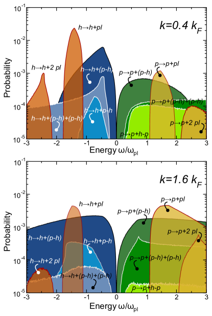
Figure 2: Monte-Carlo calculation for 3d HEG at $r_{s}=5$ density of the first and second order diagrams contributing to the electron self-energy (Eq. (26)). $\mathcal{D}_{-}^{(2b)}$ describes 3 second order processes: generation of two plasmons, of two particle-hole pairs, or of one plasmon and one particle-hole pair. The latter as well as $\mathcal{D}_{-}^{(2c)}$ are not shown because they only represent corrections to the first-order processes. The Fermi energy is set to zero.

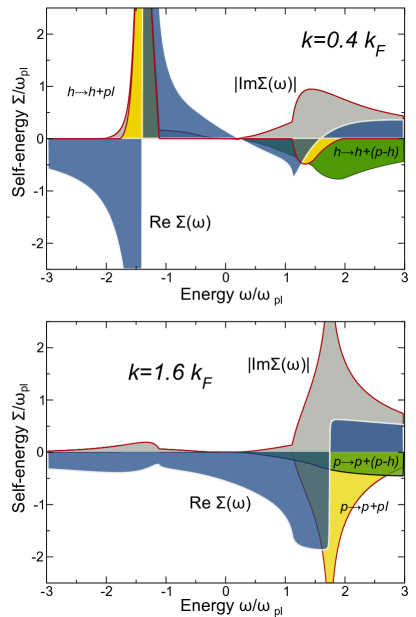
Figure 3: Exact first order self-energy of the 3d HEG at $r_{s}=5$ density. The Fermi energy is set to zero. The real part is shown without including the static (exchange) part. The values are $e_{x}=-1.490\omega_{p}$ and $e_{x}=-0.225\omega_{p}$ for $k=0.4k_{F}$ and $k=1.6k_{F}$, respectively. The plasmon energy in the long wave-length limit is $\omega_{p}=2.103\epsilon_{F}$.

In agreement with our simple argument we see that the phase-space for the first order processes is limited. The same is observed in the simplest second order process (it includes also contribution from two bare interaction lines) in view of the same arguments. The existence of a critical upper momentum for the plasmons also restricts the phase-space available for the $h\rightarrow h+2pl$ scattering. The situation is completely different for the $h\rightarrow h+(p\mathchar 45\relax h)+(p\mathchar 45\relax h)$ events: even though the hole can only loose a finite momentum the shares between the excitations can be large (Fig 1b), resulting in an arbitrarily large energy transfer (cf. Eq. (26c)). Hence, the self-energy has an unbounded support, the Paley-Wiener theorem cannot be applied and the Fermi liquid behavior is restored in the second order.

Our analysis is also important for practical calculations since it allows to determine a priori where a certain diagram might contribute. It is interesting to notice a sequence of plasmonic peaks in the see of $p\mathchar 45\relax h$ excitations. By expanding the cumulant function $C(k,t)\sim e^{i\omega_{p}t}$ (Tab. I, third column) and computing the Fourier transform one sees that their weight decays as $e^{-a}a^{n}/n!$. Guzzo et al. Guzzo et al. (2011) estimated $a\sim 0.3$ for silicon. Therefore, plasmons will only be important at low orders whereas the tails of the spectral functions are shaped by the $p\mathchar 45\relax h$ scattering mechanisms which lead to the power-law decay. Where such a crossover occurs depends, of course, on the specific system parameters.

The phase-space arguments provide a partial account of the problem. The inclusion of matrix elements can modify the self-energy substantially as the comparison of Fig. 2 and Fig. 3 shows. This can be best seen at the Fermi level (set to zero in our calculations). While both methods lead to a vanishing self-energy in this limit the way how it approaches zero is rather different. But how feasible is the realistic calculation of next order diagrams? To answer this question let us consider Eqs. (26). There, the second order terms were evaluated by using at most a 7-dimensional sampling. The full-fledged evaluation, in contrast, would require an 8-dimensional integration for each $k$ and $\omega$ values. In some specific cases simplifications might be achieved such as in exact analytic treatment of the second-order exchange term by Onsager et al. Onsager et al. (1966). On the other hand, for practical applications some synthetic approaches might be promising Takada and Yasuhara (2002); Bruneval et al. (2005).

V Conclusions

In this contribution we performed a detailed analysis of the formula $A(t;\epsilon)=A_{QP}(t;\epsilon)\,\exp\left(-\gamma(\epsilon)\frac{t^{2}}{t+\tau(\epsilon)}\right)$ for the time evolution of the spectral function for extended systems. The violations such as i) non-analyticity at short times, ii) reduction of the spectral weight of the quasiparticle peak or iii) a non-exponential decay at the long-time limit were found. Surprisingly, our theory reveals that these features are either artifacts of approximations used (iii) or are rather weak (i) as they result from rather inefficient coupling to $p\mathchar 45\relax h$ excitations. We also provide a concise analytic form for the expansion coefficients of the cumulant function at $t\rightarrow 0$.

The short-time limit was analyzed using the cumulant expansion method, while the asymptotic behavior at longer times was studied using the ordinary many-body perturbation theory. Thus, it was necessary to establish a connection between both methods. We have shown that in the first order in the screened Coulomb interaction the cumulant expansion can be recovered from the MBPT expression for the self-energy, although, some terms are additionally present in MBPT. For a finite systems we proposed a similar approach and presented results supported by full numerical calculations for Na-clusters Pavlyukh et al. (2011) and C₆₀ Pavlyukh and Berakdar (2011), which supports the general nature of the time evolution law of the spectral function. The specific, material-dependent, and quantum size effects are encapsulated in the decay constants.

Appendix A Some momentum integrals

A single momentum integral leading involving $\mathcal{D}_{-}^{(1)}(k,\omega)$ can be computed as follows:

$$\int\!d\mathbf{q}\,f(q,|\mathbf{k+q}|^{2})=\frac{\pi}{k}\int_{0}^{\infty}\!q\,dq\int_{(k+q)^{2}}^{(k-q)^{2}}\!dy\,f(q,y),$$ (27)

with $y=|\mathbf{k+q}|^{2}$. The two momenta integrals involing $\mathcal{D}_{-}^{(2a)}$ can be computed by introducing symmetrized variables as in Onsager et al. (1966):

$$\int\!d\mathbf{q}_{1}\!\!\int\!d\mathbf{q}_{2}\,f(|\mathbf{k-q_{1}-q_{2}}|^{2},\,|\mathbf{k-q_{1}}|^{2},\,|\mathbf{k-q_{2}}|^{2})\\ =\frac{1}{8}\int\!d\mathbf{q}\!\!\int\!d\mathbf{Q}\,f(|\mathbf{k-2q}|^{2},\,|\mathbf{q-Q}|^{2},\,|\mathbf{q+Q}|^{2})\\ =\frac{\pi^{2}}{8k}\int_{0}^{\infty}\!dq\int_{(k+2q)^{2}}^{(k-2q)^{2}}dy_{1}\!\!\int_{0}^{\infty}\!dQ\!\int_{qQ}^{-qQ}dy_{2}\,Q\\ \times f(y_{1},\,q^{2}+Q^{2}-2y_{2},\,q^{2}+Q^{2}+2y_{2}),$$ (28)

where

$$\mathbf{q}=\mathbf{k}-\frac{1}{2}(\mathbf{q}_{1}+\mathbf{q}_{2}),\quad\mathbf{Q}=\frac{1}{2}(\mathbf{q}_{1}-\mathbf{q}_{2});$$

$$y_{1}=|\mathbf{k}-2\mathbf{q}|^{2},\quad y_{2}=(\mathbf{q}\cdot\mathbf{Q}).$$

Analogically for the $\mathcal{D}_{-}^{(2b)}$ term we have:

$$\int\!d\mathbf{q}_{1}\!\!\int\!d\mathbf{q}_{2}\,f(|\mathbf{k-q_{1}-q_{2}}|^{2},\,|\mathbf{q}_{1}|^{2},\,|\mathbf{q}_{2}|^{2})\\ =-\frac{1}{8}\int\!d\mathbf{q}\!\!\int\!d\mathbf{Q}\,f(|\mathbf{k-2q}|^{2},\,|\mathbf{q+Q}|^{2},\,|\mathbf{q-Q}|^{2})\\ =-\frac{\pi^{2}}{8k}\int_{0}^{\infty}\!dq\int_{(k+2q)^{2}}^{(k-2q)^{2}}dy_{1}\!\!\int_{0}^{\infty}\!dQ\!\int_{qQ}^{-qQ}dy_{2}\,Q\\ \times f(y_{1},\,q^{2}+Q^{2}+2y_{2},\,q^{2}+Q^{2}-2y_{2}),$$ (29)

where

$$\mathbf{q}=\frac{1}{2}(\mathbf{q}_{1}+\mathbf{q}_{2}),\quad\mathbf{Q}=\frac{1}{2}(\mathbf{q}_{1}-\mathbf{q}_{2});$$

$$y_{1}=|\mathbf{k}-2\mathbf{q}|^{2},\quad y_{2}=(\mathbf{q}\cdot\mathbf{Q}).$$

References

- Krausz and Ivanov (2009) F. Krausz and M. Ivanov, Rev. Mod. Phys., 81, 163 (2009).
- Cavalieri et al. (2007) A. L. Cavalieri, N. Muller, T. Uphues, V. S. Yakovlev, A. Baltuska, B. Horvath, B. Schmidt, L. Blumel, R. Holzwarth, S. Hendel, M. Drescher, U. Kleineberg, P. M. Echenique, R. Kienberger, F. Krausz, and U. Heinzmann, Nature, 449, 1029 (2007).
- Schultze et al. (2010) M. Schultze, M. Fieß, N. Karpowicz, J. Gagnon, M. Korbman, M. Hofstetter, S. Neppl, A. L. Cavalieri, Y. Komninos, T. Mercouris, C. A. Nicolaides, R. Pazourek, S. Nagele, J. Feist, J. Burgdörfer, A. M. Azzeer, R. Ernstorfer, R. Kienberger, U. Kleineberg, E. Goulielmakis, F. Krausz, and V. S. Yakovlev, Science, 328, 1658 (2010).
- Ott et al. (2012) C. Ott, A. Kaldun, P. Raith, K. Meyer, M. Laux, Y. Zhang, S. Hagstotz, T. Ding, R. Heck, and T. Pfeifer, arXiv:1205.0519 (2012).
- Thygesen and Rubio (2007) K. S. Thygesen and A. Rubio, J. Chem. Phys., 126, 091101 (2007).
- Dahlen and van Leeuwen (2007) N. E. Dahlen and R. van Leeuwen, Phys. Rev. Lett., 98, 153004 (2007).
- Thygesen and Rubio (2008) K. S. Thygesen and A. Rubio, Phys. Rev. B, 77, 115333 (2008).
- Pal et al. (2009) G. Pal, Y. Pavlyukh, H. C. Schneider, and W. Hübner, Eur. Phys. J. B, 70, 483 (2009).
- Pal et al. (2011) G. Pal, Y. Pavlyukh, W. Hübner, and H. C. Schneider, Eur. Phys. J. B, 79, 327 (2011).
- Uimonen et al. (2011) A.-M. Uimonen, E. Khosravi, A. Stan, G. Stefanucci, S. Kurth, R. van Leeuwen, and E. K. U. Gross, Phys. Rev. B, 84, 115103 (2011).
- Kwong and Bonitz (2000) N.-H. Kwong and M. Bonitz, Phys. Rev. Lett., 84, 1768 (2000).
- Ness et al. (2011) H. Ness, L. K. Dash, M. Stankovski, and R. W. Godby, Phys. Rev. B, 84, 195114 (2011).
- Vogt et al. (2004) M. Vogt, R. Zimmermann, and R. J. Needs, Phys. Rev. B, 69, 045113 (2004).
- Lipavský et al. (1986) P. Lipavský, V. Špička, and B. Velický, Phys. Rev. B, 34, 6933 (1986).
- Kita (2010) T. Kita, Progress of Theoretical Physics, 123, 581 (2010).
- Nozières and De Dominicis (1969) P. Nozières and C. T. De Dominicis, Phys. Rev., 178, 1097 (1969).
- Mahan (1966) G. D. Mahan, Phys. Rev., 145, 602 (1966).
- Langreth (1970) D. C. Langreth, Phys. Rev. B, 1, 471 (1970).
- Gunnarsson et al. (1994) O. Gunnarsson, V. Meden, and K. Schönhammer, Phys. Rev. B, 50, 10462 (1994).
- Aryasetiawan et al. (1996) F. Aryasetiawan, L. Hedin, and K. Karlsson, Phys. Rev. Lett., 77, 2268 (1996).
- Guzzo et al. (2011) M. Guzzo, G. Lani, F. Sottile, P. Romaniello, M. Gatti, J. Kas, J. Rehr, M. Silly, F. Sirotti, and L. Reining, Phys. Rev. Lett., 107, 166401 (2011).
- Schork and Fulde (1992) T. Schork and P. Fulde, J. Chem. Phys., 97, 9195 (1992).
- Giuliani and Vignale (2005) G. Giuliani and G. Vignale, Quantum theory of the electron liquid (Cambridge University Press, 2005).
- Hedin et al. (1998) L. Hedin, J. Michiels, and J. Inglesfield, Phys. Rev. B, 58, 15565 (1998).
- Pavlyukh et al. (2011) Y. Pavlyukh, A. Rubio, and J. Berakdar, arXiv:1107.5632 (2011).
- Pavlyukh and Berakdar (2011) Y. Pavlyukh and J. Berakdar, J. Chem. Phys., 135, 201103 (2011).
- Paley and Wiener (1934) R. E. Paley and N. Wiener, Fourier transforms in the complex domain (American Math. Soc., New York, 1934).
- Hedin and Lundqvist (1970) L. Hedin and S. Lundqvist, in Solid State Physics, Vol. 23, edited by D. T. Frederick Seitz and H. Ehrenreich (Academic Press, 1970) pp. 1–181.
- Takada and Yasuhara (2002) Y. Takada and H. Yasuhara, Phys. Rev. Lett., 89, 216402 (2002).
- Gori-Giorgi et al. (2000) P. Gori-Giorgi, F. Sacchetti, and G. B. Bachelet, Phys. Rev. B, 61, 7353 (2000).
- Anderson (1967) P. W. Anderson, Phys. Rev. Lett., 18, 1049 (1967).
- Nozières (1994) P. Nozières, J. Phys. I, 4, 1275 (1994).
- Minnhagen (1975) P. Minnhagen, J. Phys. C, 8, 1535 (1975).
- Bose and Fitchek (1975) S. M. Bose and J. Fitchek, Phys. Rev. B, 12, 3486 (1975).
- Hedin (1965) L. Hedin, Phys. Rev., 139, A796 (1965).
- Onida et al. (2002) G. Onida, L. Reining, and A. Rubio, Rev. Mod. Phys., 74, 601 (2002).
- Aryasetiawan and Miyake (2009) F. Aryasetiawan and T. Miyake, J. Comput. Theor. Nanosci., 6, 2451 (2009).
- Ren et al. (2012) X. Ren, P. Rinke, V. Blum, J. Wieferink, A. Tkatchenko, A. Sanfilippo, K. Reuter, and M. Scheffler, New J. Phys., 14, 053020 (2012).
- Lundqvist (1967) B. I. Lundqvist, Phys. Kondens. Mater., 6, 193 (1967a).
- Lundqvist (1967) B. I. Lundqvist, Phys. Kondens. Mater., 6, 206 (1967b).
- Lundqvist (1968) B. I. Lundqvist, Phys. Kondens. Mater., 7, 117 (1968).
- von Barth and Holm (1996) U. von Barth and B. Holm, Phys. Rev. B, 54, 8411 (1996).
- Holm and von Barth (1998) B. Holm and U. von Barth, Phys. Rev. B, 57, 2108 (1998).
- Shirley (1996) E. L. Shirley, Phys. Rev. B, 54, 7758 (1996).
- Takada (2001) Y. Takada, Phys. Rev. Lett., 87, 226402 (2001).
- Note (1) See Exner (1985) and Stein and Shakarchi (2003) for a pedagogical introduction.
- Note (2) See Supplemental Material.
- Onsager et al. (1966) L. Onsager, L. Mittag, and M. J. Stephen, Ann. Phys., 473, 71 (1966).
- Bruneval et al. (2005) F. Bruneval, F. Sottile, V. Olevano, R. Del Sole, and L. Reining, Phys. Rev. Lett., 94, 186402 (2005).
- Exner (1985) P. Exner, Open quantum systems and Feynman integrals (Kluwer Academic Publishers, Dordrecht, Holland, 1985).
- Stein and Shakarchi (2003) E. M. Stein and R. Shakarchi, Princeton lectures in analysis, Vol. II Complex Analysis (Princeton University Press, Princeton, N.J., 2003).