Degenerate Convection-Diffusion Equation with a Robin boundary condition

Abstract.

We study a Robin boundary problem for degenerate parabolic equation. We suggest a notion of entropy solution and propose a result of existence and uniqueness. Numerical simulations illustrate some aspects of solution behavior.

Mohamed Gazibo Karimou

Laboratoire de Mathématiques, CNRS : UMR 6623

Université de Franche-Comte, 16, route de Gray, 25030 Besançon-France

(Communicated by the associate editor name)

1. Introduction

Let $\Omega$ be an open bounded domain of $\mathbb{R}^{\ell}$ with a Lipschitz boundary $\partial\Omega$, and $\eta$ the unit normal to $\partial\Omega$ outward to $\Omega$. The purpose of this paper is to discuss existence and uniqueness of entropy solution for the following initial boundary value problem

$$(P)\left\{\begin{array}[]{lll}u_{t}+\mathop{\rm div}f(u)-\Delta\phi(u)&=0\;\;\;\;\;\;\;\;\;\;\;\;\;\;\;\;\;\;\;\mbox{ in }\;\;\;Q=]0,T[\times\Omega,\\ u(0,x)&=u_{0}(x)\;\;\;\;\;\;\;\;\;\;\;\;\mbox{ in }\;\;\;\Omega,\\ b(u)-(f(u)-\nabla\phi(u)).\eta&=0\;\;\;\;\;\;\;\;\;\;\;\;\;\;\;\;\;\;\mbox{ on }\;\;\;\Sigma=]0,T[\times\partial\Omega.\end{array}\right.$$

Here, $u_{0}$ is taking values on $[0,u_{\max}]$ for some $u_{\max}>0$. Further, the function $f$ is a Lipschitz continuous function. Moreover, we require that

$$f(0)=0\;\mbox{ and }\;\;b(0)=0.$$ (H1)

The diffusion term $\phi$ is a continuous function. We consider that there exist a critical value $u_{c}$ of the unknown $u$ such that: $\phi(.)$ is zero on $[0,u_{c}]$ with $0\leq u_{c}\leq u_{\max}$ and $\phi(.)$ is strictly increasing else. Then problem $(P)$ degenerates to hyperbolic when $u$ takes values in the region $[0,u_{c}]$ where $\phi$ is flat.
We suppose that the function $b$ is a continuous non-decreasing function on $\Sigma$. In some situation, $b$ may be a maximal monotone graph on $\mathbb{R}$ (see [4]). Here, we assume also that $b$ satisfies the following hypotheses:

$$b=\beta\circ\phi\mbox{ where $\beta$ is a non-decreasing Lipschitz continuous function. }$$ (H2)

$$b(u_{\max})\geq|f(u_{\max}).\eta|.$$ (H3)

For more than a few decades, the degenerate parabolic equation in bounded domain was studied by many authors mainly in the case of Dirichlet boundary conditions (see e.g. [10], [8]). The zero-flux boundary condition is studied in [1] for non-degenerate parabolic case, in [7] for fully degenerate hyperbolic equation and recently in [2] for the parabolic-hyperbolic problem. Remark, that the condition $b(u)-(f(u)-\nabla\phi(u)).\eta=0$ on $\Sigma$ includes in particular Neumann (zero-flux) condition on the boundary.

We propose an adequate entropy formulation for problem $(P)$ which incorporates two boundary integrals. In [2], existence and uniqueness for the zero flux boundary condition were proved, under the assumption (H3) that reads $f(u_{\max})=0$ in the zero-flux case $b\equiv 0$. In contrast to the entropy formulation in [2], where the passage to the limit in the only boundary integral is straightforward, for our entropy inequality, we need the assumption (H2), which permits to give a sense to the boundary integral with the term $b(u)$. Indeed, we can deduce that $b(u)$ has a trace on the boundary as a function in Sobolev space $H^{1}(\Omega)$.

The proof of existence of our entropy solution for any space dimensions $\ell\geq 1$ employs a vanishing viscosity approximation. We pass to limit in the interior of the domain $Q$, by using the local compactness result of Panov [12], for this we suppose some relation between $f$ and $\phi$ (see Definition 3.5). One can refer to [2] for more details. We pay particular attention to the boundary term (here (H2) is needed).

For the uniqueness result, we use nonlinear semigroup techniques (see, e.g., [6]) and Kruzhkov doubling of variables methods. The main goal is to compare two solutions of (P), and it turns out that it is simpler to compare a solution of $(P)$ with a regular solution (in the sense that the total flux is continuous up to the boundary) of the stationary problem associated to $(P)$. Then we prove that entropy solution of $(P)$ is an integral solution, and we refer to the uniqueness of integral solutions granted by the general theory of nonlinear semigroup. Unfortunately, we are not able to obtain regular solution to the stationary problem for any space dimensions, but only in one space dimension. Then, we can deduce the uniqueness just now when $\Omega$ is a bounded open interval of $\mathbb{R}$. Notice that, for the same argument as for the zero-flux boundary condition [2], the problem of uniqueness is still open in multiple space dimensions.

The paper is organized as follows. In the next section, we give our definition of entropy solution and state some remarks useful for the well-possedness. In section 3, we prove existence result of entropy solution. In the section 4, we prove uniqueness in the case of one space dimension. The latter part is devoted to the numerical investigation of problem $(P)$. We adapt the approach of finite volumes in the spirit of Vovelle ([11]) to illustrate and interpret some observations in the case where the assumptions (H2) and (H3) are absent. Thereby, we justify the importance these assumptions in this paper.

2. Notion of entropy solution

Consider the following notion.

Definition 2.1.

A measurable function $u$ taking values on $[0,u_{\max}]$ is called entropy solution of problem $(P)$ if $\phi(u)\in L^{2}(0,T;H^{1}(\Omega))$, $b(u)\in L^{2}(0,T;H^{1}(\Omega))$ and the following conditions hold:
$\forall k\in[0,u_{\max}]$, $\forall\xi\in\mathcal{C}_{0}^{\infty}([0,T[\times\mathbb{R}^{\ell})$, with $\xi\geq 0$:

$$\displaystyle\int_{0}^{T}\int_{\Omega}\left\{|u-k|\xi_{t}+sign(u-k)\biggl{(}f(u)-f(k)-\nabla\phi(u)\biggr{)}.\nabla\xi\right\}dxdt$$

$$+\displaystyle\int_{\Omega}|u_{0}-k|\xi(0,x)dx+\displaystyle\int_{0}^{T}\int_{\partial\Omega}\left|f(k).\eta(x)-b(k)\right|\xi(t,x)d{\mathcal{H}}^{\ell-1}dt$$

$$-\displaystyle\int_{0}^{T}\int_{\partial\Omega}|b(u)-b(k)|\xi(t,x)d{\mathcal{H}}^{\ell-1}dt\geq 0.$$ (1)

Here $\mathcal{H}$ represents the $(\ell-1)-$ dimensional Hausdorff measure on $\partial\Omega$.

Remark 1.

1. The entropy solution in the sense of Definition 2.1 is in particular a weak solution. Indeed, first take in inequality (2.1), $k=0$ and use (H1). Next, take $k=u_{\max}$ and use (H3).

2. Let us stress that, in particular, the boundary condition $(f(u)-\nabla\phi(u)).\eta=b(u)$ is verified literally in the weak sense as in the case of zero flux boundary condition (see [2]). This contrasts with the properties of the Dirichlet problem (see [5]); we expect that the boundary condition should be relaxed if assumption (H3) is dropped (see [4, 3] and also numerical tests of section 5).

3. The integral in the boundary term is well defined due to the hypothesis (H2). We can use the fact that the trace of $b(u)(t,.)\in H^{1}(\Omega)$ on $\partial\Omega$ is well defined in $L^{2}(\partial\Omega)$ for $t\in(0,T)$ a.e.

According to the idea of J. Carrillo (cf [8]), we give an additional property of entropy solutions, useful for the uniqueness techniques.

Proposition 1.

Let $\xi\in\mathcal{C}^{\infty}([0,T[\times\mathbb{R}^{\ell})$; then for all $k\in[\phi_{c},u_{\max}]$; for all $D\in\mathbb{R}^{\ell}$ and for all entropy solution $u$ of $(P)$, we have:

$$\displaystyle\int_{0}^{T}\int_{\Omega}\left\{|u-k|\xi_{t}+sign(u-k)(f(u)-f(k)-\nabla\phi(u)+D).\nabla\xi\right\}dxdt$$

$$+\displaystyle\int_{\Omega}|u_{0}-k|\xi(0,x)dx-\displaystyle\int_{0}^{T}\int_{\partial\Omega}\left|b(u)-b(k)\right|\xi(t,x)d{\mathcal{H}}^{\ell-1}dt$$

$$+\displaystyle\int_{0}^{T}\int_{\partial\Omega}\left|b(k)-(f(k)-D).\eta(x)\right|\xi(t,x)d{\mathcal{H}}^{\ell-1}dt$$

$$\geq\mathop{\overline{\lim}}\limits_{\sigma\rightarrow 0}\frac{1}{\sigma}\displaystyle\int_{0}^{T}\int_{Q\cap\left\{-\sigma<\phi(u)-\phi(k)<\sigma\right\}}\nabla\phi(u).(\nabla\phi(u)-D)\xi(t,x)dxdt.$$ (2)

In general, uniqueness for evolution equation of kind $(P)$ appear very difficult mainly for the initial boundary values problems. In this context, the use of nonlinear semigroup techniques offers many advantages. Let us present briefly another notion of solution coming from the theory of nonlinear semigroups (see, e.g., [6]).

Definition 2.2.

Let $A$ be an m-accretive operator (see, e.g., [6]). Suppose that $h\in L^{1}(Q)$, $u_{0}\in L^{1}(\Omega)$. A measurable function $v\in\mathcal{C}([0,T];L^{1}(\Omega;[0,u_{\max}]))$ is an integral solution of the abstract evolution problem

$$v_{t}+A(v)\ni h(t),\;\;\;\;v(t=0)=u_{0},$$ (3)

if $v(0,.)=u_{0}(.)$ and for all $(u,z)\in A$

$$\frac{d}{dt}||v(t)-u||_{L^{1}(\Omega)}\leq\int_{\Omega}sign_{0}(v(t)-u)(h(t)-z)+\int_{\{v=u\}}|h(t)-z|\mbox{ in }\mathcal{D}^{\prime}(0,T).$$

We will see that entropy and integral solution coincide in the case $\Omega=(a,b)$ an interval of $\mathbb{R}.$

3. Existence of entropy solution

The main result of this part is the following:

Theorem 3.1.

Let $\ell\geq 1$. Assume that (H1), (H2) and (H3) holds. Suppose that $(f,\phi)$ is non-degenerate (in the sense of Definition 3.5 below). Then, there exists an entropy solution $u$ for the problem $(P)$.

To show the existence of entropy solutions, we approximate $\phi(u)$ by $\phi_{\epsilon}(u^{\epsilon})=\phi(u^{\epsilon})+\epsilon Id(u^{\epsilon})$ for each $\epsilon>0$ and set $b_{\epsilon}(u^{\epsilon})=\beta\circ\phi_{\epsilon}(u_{\epsilon})$. We obtain the following regularized strictly parabolic problem $(P_{\epsilon})$ with unknown $u^{\epsilon}$

$$(P_{\epsilon})\left\{\begin{array}[]{lll}u_{t}^{\epsilon}+\mathop{\rm div}f(u^{\epsilon})-\Delta\phi_{\epsilon}(u^{\epsilon})&=0\;\;\;\;\;\;\;\;\;\;\;\;\;\;\;\;\;\;\;\mbox{ in }\;\;\;Q=]0,T[\times\Omega,\\ u^{\epsilon}(0,x)&=u_{0}^{\epsilon}(x)\;\;\;\;\;\;\;\;\;\;\;\mbox{ in }\;\;\;\Omega,\\ b_{\epsilon}(u^{\epsilon})-(f(u^{\epsilon})-\nabla\phi_{\epsilon}(u^{\epsilon})).\eta&=0\;\;\;\;\;\;\;\;\;\;\;\;\;\;\;\;\;\;\;\mbox{ on }\;\;\;\Sigma=]0,T[\times\partial\Omega,\end{array}\right.$$

where $(u_{0}^{\epsilon})_{\epsilon}$ is a sequence of smooth functions that converges to $u_{0}$ a.e and respects the minimum/maximum values of $u_{0}$.

Definition 3.2.

Let $u_{0}$ be a measurable $[0,u_{\max}]$-valued function. A measurable function $u^{\epsilon}\in L^{2}(0,T;H^{1}(\Omega))$ taking values on $[0,u_{\max}]$ is called weak solution of problem $(P_{\epsilon})$ if : $\forall\theta\in L^{2}(0,T;H^{1}(\Omega))\cap L^{\infty}(Q)$ such that $\theta_{t}\in L^{2}(Q)$ and $\theta(T,.)=0$, one has

$$\displaystyle\int_{0}^{T}\int_{\Omega}\left\{u^{\epsilon}\theta_{t}+(f(u^{\epsilon})-\nabla\phi_{\epsilon}(u^{\epsilon})).\nabla\theta\right\}dxdt+\int_{\Omega}u_{0}^{\epsilon}\theta(0,x)dx$$

$$-\int_{0}^{T}\int_{\partial\Omega}b_{\epsilon}(u^{\epsilon})\theta d{\mathcal{H}}^{\ell-1}dt=0.$$ (4)

Theorem 3.3.

For $u_{0}\in[0,u_{\max}]$, assume (H1), (H2) and (H3) hold. Problem $(P_{\epsilon})$ admits a weak solution $u^{\epsilon}$ which is also an entropy solution. In particular, we have $0\!\leq u^{\epsilon}\!\leq u_{\max}$. In addition, there exists C independent on $\epsilon$ such that

$$||\sqrt{\epsilon}\nabla u^{\epsilon}||_{L^{2}(Q)}\leq C;$$ (5)

$$||\phi_{\epsilon}(u_{\epsilon})||_{L^{2}(0,T;H^{1}(\Omega))}\leq C;$$ (6)

$$||b_{\epsilon}^{n}(u_{\epsilon})||_{L^{1}(\Sigma)}\leq C\mbox{ and }\displaystyle\int_{\Sigma}u_{\epsilon}b_{\epsilon}^{n}(u_{\epsilon})\leq C.$$ (7)

This result can be proved, e.g., using Galerkin method (see e.g. [2]).

Lemma 3.4.

Assume that the sequence $(\Psi_{j})_{j}$ is such that: $||\Psi_{j}||_{L^{2}(0,T;H^{1}(\Omega))}\leq C$ and $\Psi_{j}\longrightarrow\Psi$ in $L^{2}(Q)$. Then $\gamma\Psi_{j}\longrightarrow\gamma\Psi$ in $L^{2}(\Sigma)$, where $\gamma$ is the trace operator.

The proof uses localization to a small neighborhood of $\Sigma$.
To prove existence of entropy solution, we assume that the couple $(f(.),\phi(.))$ is non-degenerate in the sense of the following definition:

Definition 3.5.

(Panov [12]). Let $\phi$ be zero on $[0,u_{c}]$, strictly increasing on $[u_{c},u_{\max}]$ and a vector $f=(f_{1},...,f_{\ell})$. A couple $(f(.),\phi(.))$ is said to be non-degenerate if, for all $\xi\in\mathbb{R}^{\ell}\backslash\{0\}$, the functions $\lambda\longmapsto\displaystyle\sum\nolimits_{i=1}^{\ell}\xi_{i}f_{i}(\lambda)$ are not affine on the non-degenerate sub intervals of $[0,u_{c}]$.

Theorem 3.6.

(Panov [12]). Assume that $(f,\phi)$ is non degenerate in the sense of Definition 3.5. Suppose $u^{\epsilon}$, $\epsilon>0$, is a sequence such that

$$\exists d>1,\forall s,r\in\mathbb{R}\mbox{ with }s<r$$

$$T_{s,r}(u^{\epsilon})_{t}+\mathop{\rm div}\Bigl{(}f(T_{s,r}(u^{\epsilon}))-\nabla\phi(T_{s,r}(u^{\epsilon}))\Bigr{)}\mbox{ is pre-compact in }W_{\mbox{{\tiny Loc}}}^{-1,d}(Q).$$

Moreover, suppose $u^{\epsilon}$, $f(u^{\epsilon})$, $\phi_{\epsilon}(u^{\epsilon})$ are equi-integrable locally on $Q$. Then, there exists subsequence $(u^{\epsilon})_{\epsilon}$ that converges in $L^{1}_{\mbox{{\tiny Loc}}}(Q)$.

Proof of Theorem 3.1.

(Sketched) The proof of existence of entropy solution uses Theorem 3.6 to justify the passage to the limit in $Q$ (for more details, see [2]) and Lemma 3.4 for boundary integral. ∎

4. Uniqueness result of entropy solution in one space dimension

The main result of this section is the following theorem:

Theorem 4.1.

Suppose that $\Omega=(a,b)$ is a bounded interval of $\mathbb{R}$, then $(P)$ admits a unique entropy solution.

In order to study uniqueness in the framework of nonlinear semigroup theory, we consider for all bounded function $g$ taking values on $[0,u_{\max}]$, the stationary problem $(S)$ associated to problem $(P)$:

$$(S)\left\{\begin{array}[]{rl}u+\mathop{\rm div}(f(u)-\nabla\phi(u))&=g\;\mbox{ in }\;\Omega,\\ b(u)-(f(u)-\nabla\phi(u)).\eta&=\;\mbox{ on }\;\partial\Omega.\end{array}\right.$$

The notion of entropy solution of $(S)$ correspond to the time-independent entropy solution of $(P)$ with source term $g-u$. In the case where $\Omega=(a,b)$ is a bounded interval of $\mathbb{R}$, we have an important result, which states that, the total flux is regular at the points $a$ and $b$. This kind of regularity seem hard to obtain in multiple space dimensions for $(S)$, and even in dimension $\ell=1$ for $(P)$.

Proposition 2.

For all measurable function $g$ taking values in $[0,u_{\max}]$ the problem $(S)$ admits a solution $u$ such that $(f(u)-\phi(u)_{y})$ is continuous up the boundary, i.e., $(f(u)-\phi(u)_{y})\in\mathcal{C}([a,b])$. Moreover, $b(u)-(f(u)-\phi(u)_{y}).\eta(y)$ is zero at $y=a$ and $y=b$. (Here $\eta(a)=-1$ and $\eta(b)=+1$).

From now, let’s define the operator $A_{f,\phi,b}$ on $L^{1}$ associated with regular solutions of $(S)$ by its graph:

$$(u,z)\!\in A_{f,\phi,b}=\!\left\{\begin{array}[]{ll}\!\!u\mbox{ such that }u\mbox{ is an entropy solution of }(S),\mbox{ with }g=u+z\!\!\!\end{array}\right\}\!\!.$$

Proposition 3.

1. $A_{f,\phi,b}$ is accretive in $L^{1}(\Omega)$.

2. For all $\lambda$ sufficiently small, $R(I\!+\lambda A_{f,\phi,b})$ contains $L^{1}(\Omega;[0,u_{\max}])$.

3. $\overline{D(A_{f,\phi,b})}=L^{1}(\Omega;[0,u_{\max}])$.

For the proof of this proposition, we can refer to [2].
According to the general results of [6], it follows existence and uniqueness of integral solution in the sense of Definition 2.1:

Corollary 1.

Let $\Omega=(a,b)$, $u_{0},\hat{u}_{0}\in L^{1}(\Omega)$ and $h,\hat{h}\in L^{1}(Q)$. Let $v,\hat{v}$ be integral solutions of (3) (with operator $A_{f,\phi,b}$ ) associated with the data $(u_{0},h)$ and $(\hat{u}_{0},\hat{h})$, respectively. Then for a.e. $t\in[0,T)$.

$$||v(t)-\hat{v}(t)||_{L^{1}}\leq||u_{0}-\hat{u}_{0}||_{L^{1}}+\displaystyle\int_{0}^{t}||h(\tau)-\hat{h}(\tau)||_{L^{1}}dt.$$

Adapted to our case, we have the following result

Theorem 4.2.

Let $\Omega=(a,b)$. Let $v$ be an entropy solution of $(P)$ and $u$ be an entropy solution of $(S)$. Then

$$\frac{d}{dt}||v(t)-u||_{L^{1}(\Omega)}\leq\displaystyle\int_{\Omega}sign(v-u)(u-g)dx\mbox{ in }\mathcal{D}^{\prime}(0,T).$$ (8)

In particular, $v$ is an integral solution of (3) with $h=0$.

Proof of Theorem 4.2 and Theorem 4.1.

We consider $v=v(t,x)$ an entropy solution of $(P)$ and $u=u(y)$ an entropy solution of $(S)$. Consider nonnegative function $\xi=\xi(t,x,y)$ having the property that $\xi(.,.,y)\in\mathcal{C}^{\infty}([0,T)\times\overline{\Omega})$ for each $y\in\overline{\Omega}$, $\xi(t,x,.)\in\mathcal{C}_{0}^{\infty}(\overline{\Omega})$ for each $(t,x)\in[0,T)\times\overline{\Omega}$. Apply the doubling of variables [9] in the spirit of [2], we obtain this following inequality

$$\displaystyle\int_{0}^{T}\!\!\int_{\Omega}\!\int_{\Omega}|v-u|\xi_{t}dydxdt+\displaystyle\int_{\Omega}\int_{\Omega}|v_{0}-u|\xi(0,x,y)dxdy$$

$$+\int_{0}^{T}\!\!\!\int_{\Omega}\!\int_{\Omega}sign(v-u)\Bigl{[}(f(v)-\phi(v)_{x})-(f(u)+\phi(u)_{y})\Bigr{]}.(\xi_{x}+\xi_{y})dxdydt$$

$$+\displaystyle\int_{0}^{T}\int_{x\in\partial\Omega}\!\int_{\Omega}\left|b(u)-(f(u)-\phi(u)_{y}).\eta(x)\right|\xi dyd\sigma dt$$

$$+\int_{0}^{T}\!\!\!\int_{\Omega}\!\int_{y\in\partial\Omega}\left|b(v)-(f(v)-\phi(v)_{x}).\eta(y)\right|\xi d\sigma dxdt$$

$$+\int_{0}^{T}\!\!\int_{\Omega}\!\int_{\Omega}sign(v-u)(u-g(y))\xi dydxdt$$

$$\geq\displaystyle\int_{0}^{T}\!\!\!\int_{x\in\Omega}\int_{y\in\partial\Omega}\left|b(u)-b(v)\right|\xi d\sigma dxdt+\displaystyle\int_{0}^{T}\!\!\!\int_{y\in\Omega}\int_{x\in\partial\Omega}\left|b(u)-b(v)\right|\xi d\sigma dydt$$

$$+\mathop{\overline{\lim}}\limits_{\sigma\rightarrow 0}\frac{1}{\sigma}\displaystyle\int_{0}^{T}\int\!\!\!\int_{{{\Omega_{x}^{c}}\times{\Omega_{y}^{c}}}\cap\left\{-\sigma<\phi(v)-\phi(u)<\sigma\right\}}|\phi(v)_{x}-\phi(u)_{y}|^{2}\xi dydxdt\geq 0.$$ (9)

Next, following the idea of [1], we take the test function $\xi(t,x,y)\!=\!\theta(t)\rho_{n}(x,y)$, where $\theta\!\in\!\mathcal{C}_{0}^{\infty}(0,T)$, $\theta\!\geq\!0$, $\rho_{n}(x,y)\!=\!\delta_{n}(\Delta)$ and $\Delta\!=\!(1-\frac{1}{n(b-a)})x-y+\frac{a+b}{2n(b-a)}$. Then, $\rho_{n}\in\mathcal{D}(\overline{\Omega}\times\overline{\Omega})$ and $\rho_{{n}_{|_{\Omega\times\partial\Omega}}}(x,y)=0$. Due to this choice,

$$\int_{0}^{T}\!\!\!\int_{x\in\Omega}\int_{y\in\partial\Omega}\left|b(v)-(f(v)-\phi(v)_{x}).\eta(y)\right|\rho_{n}\theta dyd\sigma dt=0.$$

By Proposition 2, $b(u)-(f(u)-\phi(u)_{y}).\eta(y)\in\mathcal{C}_{0}([a,b])$. Therefore we have
$\left|b(u)-(f(u)-\phi(u)_{y}).\eta(x)\right|\longrightarrow 0$ when $x\rightarrow y$, i.e, as $n\longrightarrow\infty$. We conclude that

$$\lim_{n\rightarrow\infty}\displaystyle\int_{0}^{T}\!\!\!\int_{x\in\partial\Omega}\int_{y\in\Omega}\left|b(u)-(f(u)-\phi(u)_{y}).\eta(x)\right|\rho_{n}\theta dyd\sigma dt=0.$$

with the calculation detailed in [2], we deduce that

$$\int_{0}^{T}\!\!\int_{\Omega}\!\int_{\Omega}\theta sign(v-u)\Bigl{[}(f(v)-\phi(v)_{x})-(f(u)-\phi(u)_{y})\Bigr{]}.\bigl{(}(\rho_{n})_{x}+(\rho_{n})_{y}\bigr{)}dydxdt\rightarrow 0.$$

Hence, we get (8) by passing to the limit in (4) with the above choice of $\xi$. Thus, the entropy solution $v$ of the problem $(P)$ is an integral solution of (3). This proves that $v$ is a unique entropy solution due to Corollary 1. ∎

5. Role of hypotheses (H2), (H3) and some numerical illustrations

The numerical analysis of $(P)$ is not the aim of this paper, although we consider this alternative in a future work. We assume (H1) holds, $u_{c}=0.6$ and $u_{\max}=1$. We present briefly the importance of the hypotheses (H2), (H3). We apply now the ideas developed e.g., in the work of Vovelle ([11]) to construct a monotone finite volume scheme which take into account the boundary condition. The interval $[0,1]$ is divided into $I$ cells. We initialize the scheme by:

$$\forall i\in\{1,...,I\}:u_{i}^{0}=\frac{1}{\delta x}\displaystyle\int_{(i-1)\delta x}^{i\delta x}u_{0}(x)dx,$$ (10)

the numerical approximation solution at $t=n\delta t$ in the cell number $i\in\{2,...,I-1\}$ is :

$$u_{i}^{n+1}\!=u_{i}^{n}\!-\frac{\delta t}{\delta x}\biggl{(}F(u_{i}^{n},u_{i+1}^{n})\!-F(u_{i-1}^{n},u_{i}^{n})\!-\frac{\phi(u_{i+1}^{n})\!-2\phi(u_{i}^{n})\!+\phi(u^{n}_{i-1})}{\delta x}\biggr{)}$$ (11)

with the boundary conditions taken into account via

$$u_{1}^{n+1}\!=u_{1}^{n}\!-\frac{\delta t}{\delta x}\biggl{(}F(u_{1}^{n},u_{2}^{n})\!-\frac{\phi(u_{2}^{n})\!-\phi(u_{1}^{n})}{\delta x}-b(u^{n}_{1})\biggr{)}.$$ (12)

$$u_{I}^{n+1}\!=u_{I}^{n}\!-\frac{\delta t}{\delta x}\biggl{(}b(u^{n}_{I})-F(u_{I-1}^{n},u_{I}^{n})\!+\frac{\phi(u_{I}^{n})\!-\phi(u_{I-1}^{n})}{\delta x}\biggr{)}.$$ (13)

Here, $F$ is a numerical flux which we assume monotone, consistent, Lipschitz continuous (see [11]). In the sequel, we take $u_{0}(x)=0.7$ if $x\in[\frac{1}{2},1]$ and $u_{0}(x)=0$ if $x\in[0,\frac{1}{2}[$. We take $\delta x=0.01$, $\delta t=\frac{\delta x^{2}}{5}$, $\phi(u)=(u-0.6)^{+}$ and consider a numerical solution at time $t=0.12$. Initially, we remove the hypothesis (H3), by taking $f(u)=\frac{u^{2}}{2}$ and $b(u)=\phi(u)$, we observe numerically the loss of maximum principle (see Figure 3 ), this mean that the the solution u can be greater than $u_{\max}$. Our entropy formulation requires to choose $b(u)$ in the functional space that permit to define the trace of $b(u)$ on the boundary. In the context where assumption (H2) is not taken into account, $b(u)=u$ and $f(u)=u(1-u)1_{[0,1]}$; numerically, we observe a boundary layer (see Figure 3 ) and this is confirmed by theoretical results of [4]. Now, taking into account assumptions (H3), (H2), with data $f(u)=u(1-u)1_{[0,1]}$; $b(u)=\phi(u)$ the numerical observation shows that the boundary condition at $x=0$ and $x=1$ is verified literally and the numerical solution respect the maximum principle (see Figure 3).

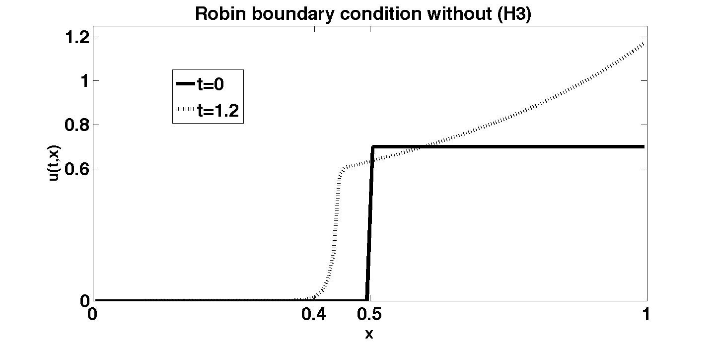
Figure 1.

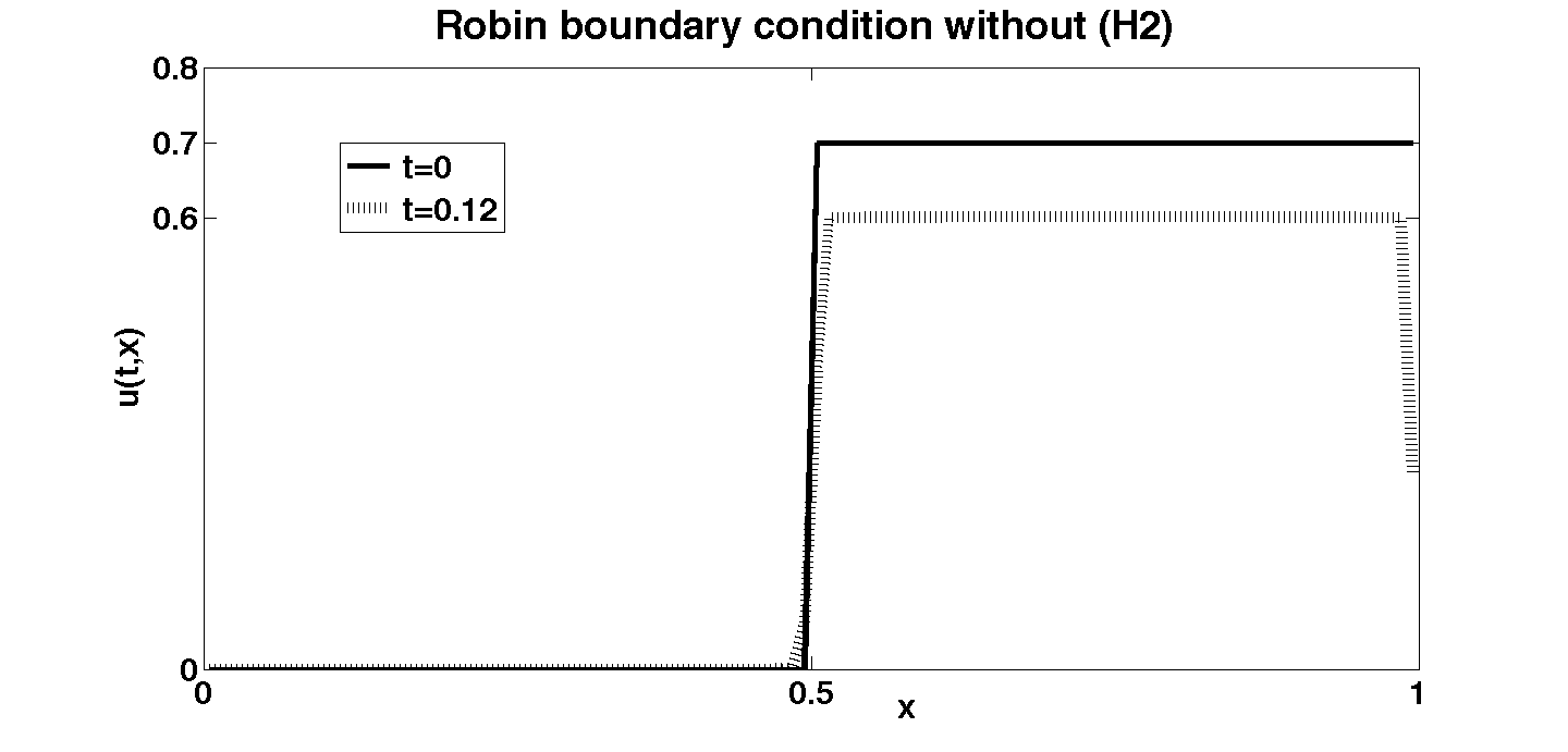
Figure 2.

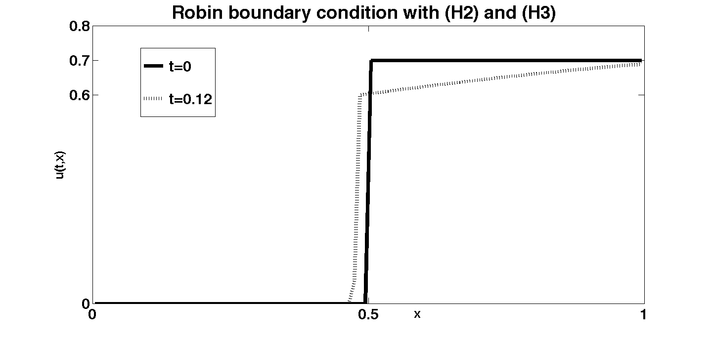
Figure 3.

References

- [1] B. Andreianov, F. Bouhsiss, Uniqueness for an elliptic-parabolic problem with Neumann boundary condition. J. Evol. Equ. 4 (2004) 273-295.
- [2] B. Andreianov, M. Karimou Gazibo, Entropy formulation of degenerate parabolic equation with zero-flux boundary condition. Z. Angew. Math. Phys., 64 (2013) no 5, pp 1471-1491.
- [3] B. Andreianov, K. Shibi, Scalar conservation laws with nonlinear boundary conditions C. R. Acad. Paris. 345 (8) (2007) 431-434.
- [4] B. Andreianov, K. Shibi, Well-posedness of general boundary-value problems for scalar conservation laws. Trans. AMS, accepted. Available as preprint HAL http://hal.archives-ouvertes.fr/ : hal-00708973, version 2.
- [5] C. Bardos, A.Y. Le Roux, J.C. Nedelec, First order quasilinear equations with boundary conditions. Comm. PDE. 4 (1979) 1017-1034.
- [6] Ph. Bénilan, Crandall, M. G. and Pazy, A., Nonlinear evolution equations in Banach spaces. Preprint book.
- [7] R. Bürger, H. Frid, K. H. Karlsen, On the well-posedness of entropy solution to conservation laws with a zero-flux boundary condition. J. Math. Anal. Appl. 326 (2007), 108-120.
- [8] J. Carrillo, Entropy solutions for nonlinear degenerate problems. Arch. Ration. Mech. Anal. 147 (4) (1999) 269-361.
- [9] S.N. Kruzkhov, First order quasi-linear equations in several independent variables. Math. USSR Sb. 10 (2) (1970) 217-243.
- [10] C. Mascia, A. Porretta, A. Terracina, Nonhomogeneous Dirichlet problems for degenerate parabolic-hyperbolic equation. Arch. Ration. Mech. Anal. 163 (2) (2002) 87-124.
- [11] J Vovelle, Convergence of finite volume monotones schemes for scalar conservation laws on bounded domains. Numer. Math., 90, (3), (2002) 563-596.
- [12] E.Yu. Panov, On the strong pre-compactness property for entropy solutions of a degenerate elliptic equation with discontinuous flux. J. Differential Equations. 247 (2009) 2821-2870.