Bootstrapping under constraint for the assessment of group behavior in
human contact networks

Abstract

The increasing availability of time – and space – resolved data describing human activities and interactions gives insights into both static and dynamic properties of human behavior. In practice, nevertheless, real-world datasets can often be considered as only one realisation of a particular event. This highlights a key issue in social network analysis: the statistical significance of estimated properties. In this context, we focus here on the assessment of quantitative features of specific subset of nodes in empirical networks. We present a method of statistical resampling based on bootstrapping groups of nodes under constraints within the empirical network. The method enables us to define acceptance intervals for various Null Hypotheses concerning relevant properties of the subset of nodes under consideration, in order to characterize by a statistical test its behavior as “normal” or not. We apply this method to a high resolution dataset describing the face-to-face proximity of individuals during two co-located scientific conferences. As a case study, we show how to probe whether co-locating the two conferences succeeded in bringing together the two corresponding groups of scientists.

I Introduction

High resolution measurements of co-presence and even face-to-face interactions between individuals in different social gatherings – such as scientific conferences, museums, schools, or hospitals – were made possible in the recent years by the use of wearable sensors, using bluetooth, wireless or RFID (Radio Frequency IDentification) technology. These new data paved the way to many empirical investigations Cattuto et al. (2010); Eagle and Pentland (2006); Hui et al. (2005); Salathé et al. (2010) of human contacts, both from a static (e.g., existence of communities, clustering, heterogeneities in the number of contacts…) and dynamic (distribution of the durations of contacts, of the time between contacts, or of the lifetime of groups of different sizes…) points of view.

A major issue regarding the analysis of these datasets is that each one of them represents a single realisation of a particular event: in contrast to the study of ensembles of random networks, it is not possible to generate multiple realizations of the event. Associating a statistical significance to any measured property of these datasets is thus a challenging issue. The present work seeks to attribute statistical significance, in the form of a statistical test and acceptance intervals, to observable features in a network. More precisely, the features under study will characterize a specific group of nodes within the graph, and we discuss how to address the question whether this group of nodes is normal or not as compared to other groups in the network.

Two data-driven methods have been widely used in the general case to obtain acceptance intervals for observable features: the jackknife and bootstrapping Efron (1982); Zoubir and Iskander (2004). Both are based on drawing random samples from the unique original data recorded in an observation. Transposing the classical bootstrap approach to the case of data represented by graphs is however not straightforward. Only a few works have considered resampling of graphs, for instance via the generation of resampled versions of the empirical graph as a whole Eldardiry and Neville (2008); Ying and Wu (2009). Classically, graph resampling methods aim at studying the significance of the empirical graph structure and topology, for instance for phylogenetic trees Drummond and Rambaut (2007) or bayesian-induced networks Friedman et al. (1999). Another application concerns the significance of community structures Fortunato (2010); Lancichinetti et al. (2010); Rosvall and Bergstrom (2010) in networks. Here, in contrast with these works, we do not perform graph resampling as we consider the whole network as a fixed input: our aim is to use statistical resampling techniques to design a statistical test and acceptance intervals for observables pertaining to groups of nodes in a given (empirical) network.

In this paper, focusing on features of groups of nodes, we formulate a bootstrap protocol suited to complex networks. To this aim, we focus on a specific group of nodes in the graph, consider resampled versions of this group of interest within the graph, and compare the studied group with its resampled versions. A key point is that the resampled groups have to take into account some dependences or constraints existing in the original group in order to constitute a relevant bootstrap ensemble. We then choose specific group features and compare these features in the original group and in the resampled groups. This procedure provides a measure of the statistical significance of the chosen features in the graph. The developed method allows us to estimate whether a feature deviates from a normal behavior of this feature in the bootstrap ensemble (i.e., a Null Hypothesis of a statistical test for this feature). By combining several features, it enables us to define normal behaviors of groups of nodes in the graph and to assess whether the specifically studied group’s behavior is normal or anomalous, and in which respect.

The paper is structured in the following way. We introduce in Section II the bootstrapping of groups of nodes in complex networks and how to use this procedure to devise statistical tests; this part represents the methodological contribution of this work. Then, in order to illustrate the possibilities offered by the proposed method for real data of complex networks, we consider a dataset describing the face-to-face interactions of individuals collected in two co-located conferences of the American Physical Society, involving two distinct scientific groups: the Division of Plasma Physics Meeting and the Gaseous Electronics Conference. We show in Section III how the proposed method assesses to what extent both groups mix together during these conferences. A conclusion is given in Section IV. Details on the data set as well as on a validation of our method on controlled benchmarks are provided in the Appendices.

II Bootstrapping and statistical test for complex networks

Our main objective is to provide statistical significance for measured features associated to subsets of nodes (’groups’) in networks. A standard way is to formulate a Null Hypothesis for the normal behavior of a group, and to perform a statistical test to decide whether or not this Null Hypothesis has to be rejected. In this section, we will propose in the context of weighted networks a specific resampling method based on bootstrapping constrained groups in the network, and a way to perform statistical tests using this bootstrapping method.

Bootstrapping Efron (1982); Zoubir and Iskander (2004) is a well-known data-driven method that creates new random pseudosamples by using only one empirical observation of the data. In order to adapt the bootstrapping methodology to our goal, we propose here a specific resampling method to draw replicates of groups with relevant properties. The method is based on two main ingredients: 1) to describe normal behavior, a Null Hypothesis is defined that imposes constraints on the groups and we propose a computational scheme to draw groups that correspond to the proposed Null Hypothesis; 2) we build a bootstrap set of many such constrained groups, by randomly sampling them independently and with replacement, as in classical bootstrapping. Combining these two steps, we are then able to propose a bootstrap test to decide whether the specific group of interest is compatible with the proposed Null Hypothesis. We detail the method in the next paragraphs.

The main advantage of using a bootstrap-inspired technique is that it does neither require any additional information with respect to the network itself, nor any model of the network’s properties: it is fully data-driven. Moreover, unlike other data-driven resampling methods such as the jackknife, it is possible to adjust the size of the drawn samples to the size of the studied group.

However, a major and tricky issue arises when assessing significance of some features of a specific group in a network: generally, neither the nodes nor the links are independent from each other. Simple use of descriptive statistics of classical bootstraps are not suited to deal with dependent data. A key point of our work is to propose a protocol suited to networks, that takes into account some of the dependences in the data.

II.1 Relevant observable features for groups in complex networks

Let $\mathcal{G}=(\mathcal{V},\mathcal{E})$ be the graph representation of the studied complex network, with $\mathcal{V}$ its set of nodes and $\mathcal{E}$ its set of edges. We call $X^{0}\subset\mathcal{V}$ the chosen subset of nodes whose behavior we want to compare to the behavior of “normal” groups, obtained as random bootstrap samples satisfying given constraints as explained above. Let us call $R^{0}\subset\mathcal{V}$ the remaining nodes of the network ($R^{0}=\mathcal{V}\backslash X^{0}$).

We quantify $X^{0}$’s “behavior” by looking at several observable features that are representative of how the group is structured. In the context of social networks, relevant features are for instance ones that quantify whether there are strong contacts inside the group, possibly stronger than with other nodes. For the use of the method in Section III, the following observable features are used (generically referred to as $Z^{0}$ in the following), in addition to the cardinality $M$ of the group $X^{0}$:

• $N_{XX}^{0}$ the total number of links of $\mathcal{E}$ between nodes of $X^{0}$;

• $N_{RR}^{0}$ the total number of links of $\mathcal{E}$ between nodes of $R^{0}$;

• $N_{XR}^{0}$ the total number of links of $\mathcal{E}$ connecting the two groups of nodes;

• $T_{XX}^{0}$ the total weight of the links of $\mathcal{E}$ between nodes of $X^{0}$;

• $T_{RR}^{0}$ the total weight of the links of $\mathcal{E}$ between nodes of $R^{0}$;

• $T_{XR}^{0}$ the total weight of the links connecting the two groups.

• $Q_{X}^{0}$ the modularity computed when partitioning the nodes of $\mathcal{G}$ in two groups $X^{0}$ and $R^{0}$.

For completeness, we recall that the modularity of a partition of $\mathcal{G}$ is defined by Newman (2004): $Q=\frac{1}{2N}\sum_{i\in\mathcal{V},j\in\mathcal{V}}\left[A_{ij}-\frac{s_{i}s_{j}}{2N}\right]\delta(c_{i},c_{j})$, where $A$ is the weighted adjacency matrix of the graph $\mathcal{G}$, $s_{i}=\sum_{j\in\mathcal{V}}A_{ij}$ is the strength of node $i$, $N=\frac{1}{2}\sum_{i\in\mathcal{V},j\in\mathcal{V}}A_{ij}$ is the sum of all weights, and $c_{i}$ is the label of the group of node $i$, so that $\delta(c_{i},c_{j})=1$ if nodes $i$ and $j$ are in the same group, and $0$ otherwise. In the present case of a partition in two groups, the modularity takes values between $-0.5$ and $0.5$ and measures how well the partition separates the network into distinct communities (a value close to $0.5$ denotes two strong communities) .

We thus consider overall $F=7$ observables features (in addition to the cardinality of the group). The chosen observables are not fully independent and one might question why we consider so many. In particular, one of the most widely used observables regarding the behavior of a group in a network is the modularity Newman (2004), and one might argue that is is enough to consider cardinality and modularity; however, modularity is neither a sufficient nor a unique way to discriminate between different types of behaviors. Moreover, the studied groups (i.e., of which one wants to know if they are normal or not) might not necessarily form communities in the network. By adding the six other observables that are admittedly not totally independent from the modularity, we accept some level of redundancy in the information we gather in order to yield a more complete and discriminative description of groups.

Depending on the specific issue addressed and of the nature of the complex network at hand, other observable features could be considered as relevant to describe the behavior of a group. We are here guided by the case study we will consider later, consisting in networks of face-to-face contacts between individuals (details on the data are given in the next Section and in Appendix C), but we emphasize that the proposed procedure of bootstrap under constraints is directly usable in other contexts.

II.2 Bootstrapping protocol for statistical testing of a group in a network

Once the $F$ specific features $Z$ are chosen ($Z$ is used as a generic notation for any one feature, while $Z^{0}$ is the value taken by this feature for the group of interest), the steps forming the backbone of the bootstrapping procedure to test the normality of a group in a network are as follows:

1. First, we formulate a Null Hypothesis regarding what is supposed to be a “normal” behavior of $X^{0}$ in the network. This Null Hypothesis is defined as a specific set of constraints on the groups that obey this supposedly “normal” behavior. More specifically, a relevant constraint will be that a given feature $Z$ takes the value $Z^{0}$ for each of these groups. Let us note $f$ the number of features that are constrained by the Null Hypothesis.

2. Second, we create a bootstrap set of $N_{B}$ constrained groups by sampling with replacement from the data groups of nodes satisfying the constraints of the Null Hypothesis; we use $X$ as a generic notation for the bootstrap samples. In some cases, in order to obtain enough different samples, we will need to relax some constraints of the Null Hypothesis: such a relaxed constraint on a feature $Z$ is then written as $Z^{0}(1-\delta)\leq Z\leq Z^{0}(1+\delta)$. The value of $\delta>0$ tunes the strength of the constraint (the choice of $\delta$ is discussed in Section II.5). The sampling procedure, based on simulated annealing, is described in details in Appendix A.

3. For large enough $N_{B}$, we estimate the distribution of each feature for the groups in the bootstrap set. These distributions describe in a fully data-driven way the “normal behavior” of groups in the empirical network under the chosen Null Hypothesis (i.e., under this particular set of $f$ constraints).

4. We select a significance level $\alpha$ for testing the Null Hypothesis, i.e., the probability to reject the Null Hypothesis even if it is true has to be less than or equal to $\alpha$. $\alpha$ will also be called false alarm rate in the following. In the litterature, it is also called probability of false detection Barnes et al. (2009). Because we are dealing with observable features $Z$’s that are possibly dependent, the Bonferroni correction is employed: a significance level $\alpha^{\prime}=\alpha/(F-f)$ is defined and used to test the $F-f$ individual features that are not constrained by the Null Hypothesis (See Section II.3).

5. To decide whether or not we can reject the Null Hypothesis with a significance level $\alpha$, and how far from the Null Hypothesis the group of interest is, a suitable divergence $d$ (defined in Section II.3) is computed from the $Z^{0}$’s and the empirical distributions of the $Z$’s for the bootstraps. When $d=0$, the Null Hypothesis cannot be rejected with a significance level $\alpha$; when $d$ is higher, it evaluates to what extent $X^{0}$ deviates from the bootstrap samples and from the formulated Null Hypothesis, hence from the supposed “normal behavior”.

6. As a final output, two indicators of the size of the bootstrap space are computed (defined in II.4) to check whether the constraints with the relaxation factor $\delta$ remain relevant enough for the Null Hypothesis to be tested, as further discussed in II.5.

II.3 Normalization of features, test of individual features and choice of the divergence $d$

Each observable $Z$ is normalized into a dimensionless quantity $z$ known as the “Z-score”: $z=(Z-\bar{Z^{*}})/\sigma_{Z}^{*}$ where $\bar{Z^{*}}$ is the expected value and $\sigma_{Z}^{*}$ the standard deviation of the observable $Z$ in a random graph with the same weight sequence as the empirical data. To estimate these values, the following procedure is considered. Random graphs are obtained by randomly re-allocating the weights from the full weight sequence (including the zero weights, corresponding to absent links), within the ensemble of possible links (i.e., pairs of nodes). This randomizes the degree of the nodes as well as their strengths (the strength is defined as the sum of the weights of the links of a node) and the local topological structures, and only preserves the weight sequence. $\bar{Z^{*}}$ and $\sigma_{Z}^{*}$ are computed as the average and the standard deviation over the ensemble of such random graphs. This normalization may seem arbitrary, but this mode of representation is chosen for its clarity (we can plot the results for all $F=7$ observables on the same scale) and, more importantly, it allows us to compare the results between groups of different sizes.

For each normalized observable $z$, the empirical distribution function $\hat{D}_{z}^{b}$ is derived from the bootstrap set. As mentioned above, a statistical test is then performed on $X^{0}$ for the $z$’s to decide if $X^{0}$ appears as statistically far from the bootstrap set of not. The significance level $\alpha$ of the test cannot be used directly in this case, as we are in a situation of multiple tests (the number of tests is $F-f$ as $f$ features are constrained by the Null Hypothesis). As the tests against the various features are not necessarily independent, the Bonferonni correction is used: this correction states that if we test each feature with a significance level $\alpha^{\prime}=\alpha/(F-f)$, the whole family of tests (i.e., the combined test for all the features) holds under a significance level $\alpha$ (which would be a pessimistic, higher bound of the true false alarm rate). Hence, the Null Hypothesis is rejected for a specific feature $z$ if $z^{0}$ (the actual measured value for $X^{0}$) is outside the $1-\alpha^{\prime}$ two-sided acceptance interval for $\hat{D}_{z}^{b}$.

We finally define a divergence $d$ quantifying if $X^{0}$ is far from the bootstrap set of not. For each observable feature $Z$, we define $d_{z}$ as the minimum distance between $z^{0}$ and the $1-\alpha^{\prime}$ two-sided acceptance interval for $\hat{D}_{z}^{b}$. If $z^{0}$ is in the interval, $d_{Z}=0$. As this interval has the meaning of an acceptance interval for the Null Hypothesis for this feature, $d_{z}$ measures the deviation of the observed value $Z^{0}$ for $X^{0}$ from the Null Hypothesis.

We then consider the sum $d$ of the divergences $d_{z}$ as the global divergence measuring to what extent we have to reject the Null Hypothesis for $X^{0}$: if $d$ is larger than 0, the Null Hypothesis is rejected for the group $X^{0}$ with a significance level $\alpha$ and the larger is $d$, the further away is the group $X^{0}$ from the Null Hypothesis. If $d$ equals 0 on the other hand, there is no reason to reject the Null Hypothesis under the significance level $\alpha$.

II.4 Outputs of the constrained bootstrap method

In classical unconstrained bootstrap, the relevance of the test relies on an unbiased randomness in the drawing of the samples Zoubir and Iskander (2004). In the present case, by imposing constraints on the bootstrap samples, some randomness is lost and this introduces possible dependencies: while the divergence $d$ is sufficient to summarize an unconstrained test’s outcome, we need here to track the bias introduced by the constraints. In the following, we propose a practical way to check the validity of the procedure.

We consider two indicators to monitor the bias introduced by the constraints. The first one is the standard deviation $\sigma_{u}$ of the distribution of the number of times each node is chosen in a bootstrap sample. It measures how uniformly a node is chosen in a bootstrap sample: the smaller is $\sigma_{u}$, the more the choice of the nodes for the bootstrap set is uniform. The second indicator measures if nodes in $X^{0}$ are chosen more – or less – often in the bootstrap samples than they would if there were no constraints. To this aim, we compare the empirical distribution of the number of nodes from $X^{0}$ that are in a bootstrap sample to the theoretical distribution that would emerge if there were no constraints. This theoretical probability distribution is the one of drawing $k$ nodes from $X^{0}$ after $M=|X^{0}|$ draws without replacement in a set of $V=|\mathcal{V}|$ nodes: it is given by the hypergeometric law $P(k)={{{M\choose k}{{V-M}\choose{M-k}}}\over{V\choose M}}$. We thus compute the $\chi^{2}$ distance between the empirical distribution and the theoretical hypergeometric distribution. In order to compare different $\chi^{2}$ obtained from different bootstrap tests, each $\chi^{2}$ value is computed with 10 bins that contain at least five realisations. An important point is that we do not use $\chi^{2}$ for a goodness-of-fit test. We indeed expect $\chi^{2}$ to increase as soon as we impose strong constraints on the bootstrap samples. Rather, we use $\chi^{2}$ and $\sigma_{u}$ as two control parameters of the “uniform character” of the bootstrapping procedure, and check that they stay reasonably small.

Overall, the final output of the proposed test is a triplet $(d,\chi^{2},\sigma_{u})$ that sums up the outcome of the test for $X^{0}$, under the two parameters given by the significance level $\alpha$ and the relaxation factor $\delta$ for the constraints. The larger is $d$, the further away the group is from the Null Hypothesis. The smaller $\chi^{2}$ and $\sigma_{u}$, the less biased is the choice of the bootstrap set.

II.5 Trade-off between the constraint(s) strength and the statistical power of the test

The parameter $\delta$ tunes the “strength” of a given constraint: the lower $\delta$, the stronger the constraint. Consider a very strong constraint (with a small parameter $\delta$). In this case, the space of possible bootstraps may be drastically reduced to the point where the only possible bootstraps that verify the constraint are very similar to the tested group $X^{0}$. The test will then naturally be unable to reject the Null Hypothesis ($d=0$) even if $X^{0}$ is abnormal (i.e. the test has a low statistical power)! In other words, consider an abnormal group $X^{0}$. One can always find a constraint (or a set of constraints) strong enough that will classify $X^{0}$ as normal. There is therefore a minimal value of $\delta$ under which the test loses its power.

On the other hand, the point of developing a method of bootstrapping under constraint is to test groups with highly specific Null Hypotheses, and to be able to understand precisely why a group is abnormal or not. We therefore want $\delta$ to be as small as possible in order to have bootstraps as representative of the Null Hypothesis as possible.

Hence, for each given constraint, there exists a trade-off value $\delta^{*}$ of $\delta$ that maximizes both the power and the precision of the test. The existence of a threshold value $\delta^{*}$ for $\delta$ transposes in the existence of maximum authorized values $\chi^{2*}$ and $\sigma_{u}^{*}$.

In order to carry out the procedure outlined in this Section, we thus need to estimate $\delta^{*}$, $\chi^{2*}$ and $\sigma_{u}^{*}$. A theoretical estimation remains an open question . We therefore use a controlled graph model, for different types of constraints and different cardinality of groups, and estimate in each case the corresponding threshold values. Details and results are exposed in Appendix B, and we will use in the following the values of $\delta^{*}$, $\chi^{2*}$ and $\sigma_{u}^{*}$ obtained in this way.

To sum up the discussion, the test has three possible outputs:

1. $d>0,\forall(\chi^{2},\sigma_{u})$. In this case where $d>0$, there is no need to discuss the values of $\chi^{2}$ and $\sigma_{u}$. Indeed, even if $\chi^{2}>\chi^{2*}$ and/or $\sigma_{u}>\sigma_{u}^{*}$, i.e., even if the bootstraps seem too similar to $X^{0}$, $X^{0}$’s behavior is still observed to be different than the bootstraps: the Null Hypothesis is rejected.

2. $d=0,\chi^{2}<\chi^{2*},\sigma_{u}<\sigma_{u}^{*}$. The bootstrap space is large enough, the test maintains its statistical power: the Null Hypothesis is not rejected.

3. $d=0,\chi^{2}>\chi^{2*}$ and/or $\sigma_{u}>\sigma_{u}^{*}$. In this case, we are in the situation discussed above: the test is not powerful enough and no conclusion can be made.

III Case study: bootstrapping under constraints for specific groups of attendees in the conference

In order to illustrate our procedure, we consider a dataset describing the face-to-face proximity of individuals, collected in Salt Lake City (SLC) in November 2011 during two co-located scientific conferences lasting five days. These conferences were jointly organised by the DPP (Division of Plasma Physics) of the American Physical Society and the GEC (Gaseous Electronics Conference) in an attempt to bring together both groups – mainly academic researchers and engineers, respectively. A description of the context, the data collection procedure and the dataset is provided in Appendix C. We provide in Table 1 some basic statistics of the data. Note that the sum of the total number of contacts (and the total time of contact) within DPP and within GEC does not exactly account for the interactions for the conference taken as a whole (ALL), due to the interactions between DPP and GEC. We will consider here the aggregated network of face-to-face proximity between individuals, in which each node represents an individual and where the weight of a link between two individuals gives the cumulated time they have spent in face-to-face interaction during the conference. Moreover, we pre-process the obtained contact network by deleting links between nodes that correspond to an aggregated contact time of the two corresponding individuals smaller than $1$ minute over the whole conference. The threshold of $1$ minute is chosen because smaller contact times can be considered as noise in the measurement, associated to very short contacts. We have checked that our results are robust with respect to the filtering threshold: similar results are obtained when thresholding at $3$ and $5$ minutes.

	SLC
	GEC	DPP	ALL
No. of tags	39	281	320
sample rate	12%	16%	15%
No. of days	5
No. of contacts	1189	21519	23920
Tot. time of contact (hours)	18	306	339

Table 1: Basic statistics concerning the datasets collected in the co-located scientific conferences.

The original question of interest for the organizers of the SLC conferences is whether co-locating both conferences was worthwhile, i.e., whether the GEC and DPP groups mixed together. In order to give a quantitative answer to the question, one needs to compare the amount of interactions between GEC and DPP to some reference. To this aim, the proposed bootstrap method is a natural candidate.

III.1 Choosing the groups and the Null Hypotheses

The $F=7$ chosen observable features that characterize a group’s “behavior” include features measured within the group ($N_{XX}$ and $T_{XX}$), features measured within the rest of the network ($N_{RR}$ and $T_{RR}$), and features measuring the interaction between the group and the rest of the network ($N_{XR}$, $T_{XR}$ and $Q_{X}$). The terminology “group’s behavior” is used for simplicity, but the chosen features quantify also the behavior of the group’s complementary as well as the interaction of the group with the rest of the network. Quantifying for instance “GEC’s behavior” represents therefore a possible measurement of the mixing between both groups, as the DPP individuals correspond precisely to the “rest” of the network. The method previously exposed is a means not only to quantify, but also to validate statistically, the normality – or abnormality – of GEC’s behavior with respect to various Null Hypotheses. We thus use this method for the group of GEC individuals, taken as the specific subset of interest $X^{0}$ in the face-to-face contact network between the attendees of the SLC conference. All the statistical tests reported afterwards are done under a significance level $\alpha=5\%$.

It is difficult to decide on only one specific Null Hypothesis that should describe the expected behavior of a given group during the conference. There are few models for the dynamics of face-to-face contacts (e.g., Stehlé et al. (2010); Zhao et al. (2011); Starnini et al. (2013)), and none has been designed to account for all the possible features of groups in a social network, so that we can not simply compare the results of such models with our data. The proposed bootstrap method allows here for an interesting approach: instead of deciding on an arbitrary Null Hypothesis, we can test the behavior of the GEC group against various Null Hypotheses that can be formulated. The objective of the study is not merely in knowing if the GEC group was different from other groups in the conference, but in knowing in which respect GEC is (or is not) different from other groups in a statistically significant manner.

The different Null Hypotheses on which we will use the bootstrap statistical tests are taken as constraints on the amount of interaction involving nodes of $X$. We will consider several different Null Hypotheses, or sets of constraints: in each case, the Null Hypothesis can be phrased as “$X^{0}$ has a behavior compatible with a random group $X$ of nodes satisfying the chosen set of constraints”. The considered sets of constraints defining these Null Hypotheses are:

• the size of the group is fixed, equal to the one of $X^{0}$; this constraint is always active, so that there is no effect due to the variation of the size of the group. As there are no constraints on the chosen features, $f=0$.

• the modularity of the partition of the network between the group and its complement is equal to the one of the partition $(X^{0},{\cal V}\backslash X^{0})$, up to a relaxing factor $\delta$. Note that here $f=1$ to compute $\alpha^{\prime}=\alpha/(F-f)$.

• constraints are put on $N_{XX}$ or $T_{XX}$, imposing that they take the same values as respectively $N_{X^{0}X^{0}}$ or $T_{X^{0}X^{0}}$ (still in addition to the cardinality constraint). These constraints correspond to ways of imposing a certain number of links or a certain amount of interaction within the group. Here again, $f=1$.

Moreover, it is possible that all groups with a community behavior (as given quantitatively by the seven features) could appear as abnormal. We thus investigate the case of three other specific groups of individuals that might a priori present a community behavior: the Students from DPP, i.e. attendants preparing a PhD thesis (STP), the Juniors from DPP, i.e. researchers with less than 10 years of professional experience (JUP), and the Seniors from DPP, i.e. researchers with more than 10 years of experience (SEP). Table 2 summarizes the measured features for the GEC, STP, JUP and SEP. One could expect each of these group to form a community in the contact network because of the similarities of their members in age and professional status. When partitioning the network into one of these groups and its complement, the modularity presents indeed a high enough value. It is therefore sound to compare the tests’ outputs for GEC and for these other groups: if their behavior is similar, it could be argued that the subgroup GEC simply behaves as if it were a subgroup of interest of DPP, and the conclusion would be that the co-location of the conference was an efficient way to bring together GEC and DPP. If instead GEC is significantly more abnormal than the three other groups, one may doubt the efficiency of the co-location.

Group	Cardinality	$N_{XX}$	$N_{XR}$	$N_{RR}$	$T_{XX}$	$T_{XR}$	$T_{RR}$	$Q_{X}$
GEC	39	101	120	1907	58820	45740	947100	0.100
STP	106	384	850	894	252900	356220	442540	0.145
JUP	73	183	766	1179	97600	303800	650260	0.073
SEP	99	226	704	1198	124280	310740	616640	0.095

Table 2: The cardinality and the other seven features of the four groups under study. The temporal quantities $T_{XX}$, $T_{XR}$ and $T_{RR}$ are given in seconds.

Our approach is therefore to test those four groups (i.e., the group noted $X^{0}$ in the method will alternatively be GEC, STP, JUP, or SEP) against the same Null Hypotheses and to compare the degree with which the Null Hypotheses are rejected for each group.

III.2 Results

We first consider the simple cardinality constraint. More precisely, we test if GEC behaves like any random group of $M=39$ individuals in the conference. As could be expected, the corresponding Null Hypothesis is rejected, which does not come as a surprise given the quite large value of $Q_{X}$. In fact, the Null Hypothesis is as well rejected for the three other groups (SEP, JUP, STP), which means that this simple constraint does not allow us to assert if GEC behaves differently from these other groups. Details on the procedure and its outcome are provided in Appendix D.

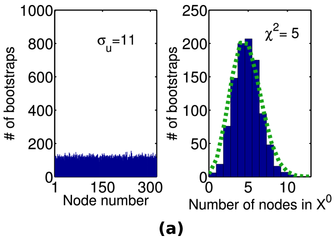
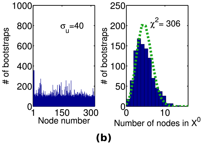
Figure 1: Outputs $\sigma_{u}$ and $\chi^{2}$ of the bootstrap method for $X^{0}$ = GEC for (a) test with the same cardinality constraint (further detailed in Appendix D), (b) test with the constraints of same cardinality and same modularity (with $\delta=15\%$). Left: histogram of the number of occurrences of each node in the bootstrap samples and its standard deviation $\sigma_{u}$. Right: histogram of the number of $X^{0}$-nodes in a bootstrap sample with its $\chi^{2}$ distance from the theoretical hypergeometric histogram (dotted line).

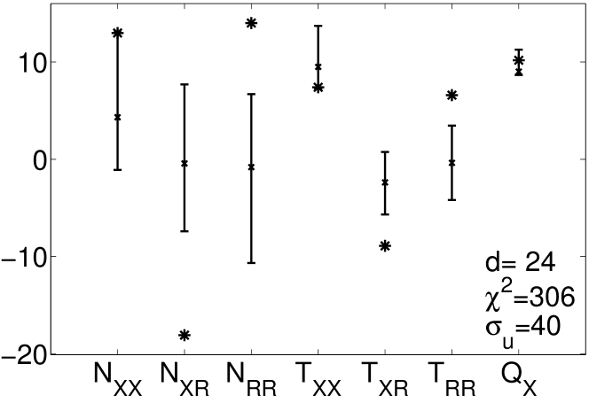
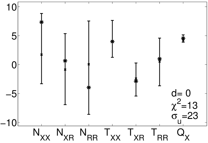
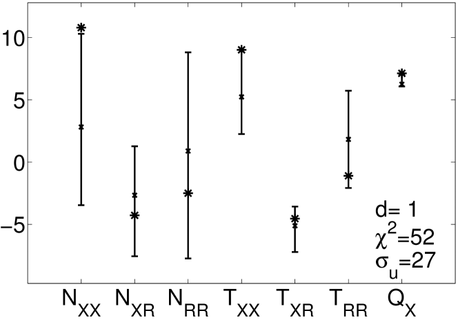
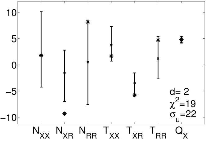
Figure 2: Results of the test with the constraints of fixed cardinality and fixed modularity (with $\delta=15\%$) for the four groups: GEC (top left), STP (top right), JUP (bottom left), and SEP (bottom right). For each $z$, the two-sided acceptance interval with $1-\alpha^{\prime}$ significance level is in black and the value $z^{0}$ is shown as a black star. Here, $\alpha=5\%$, i.e. $\alpha^{\prime}=\frac{\alpha}{F-f}=\frac{0.05}{6}=0.8\%$. For each group $X^{0}=$ GEC, STP, JUP and SEP, the scalar $d$ (bottom right hand corner of each figure) is the total divergence between the acceptance interval of the bootstrap samples and the real data. $\chi^{2}$ and $\sigma_{u}$ are the two control parameters of the size of the bootstrap space.

In order to better discriminate GEC’s behavior from the behavior of other groups, we therefore turn to more refined Null Hypotheses, i.e., with stronger constraints on the bootstrap samples. As discussed in Section II.5 and Appendix B.3, the parameter $\delta$ is set to the threshold value $\delta^{*}$ corresponding to the type of constraint considered (see Table 4).

The first refined Null Hypothesis that we consider accounts for the high modularity of $X^{0}$: does $X^{0}$ behave like any random group of nodes of same cardinality and modularity as $X^{0}$ (hence forming a community as strong as $X^{0}$)? This latter constraint on modularity is relaxed with $\delta^{*}=15\%$, according to the simulations of Appendix B.3.

Figure 1 displays, in a) for the simple cardinality constraint and in b) for the present case, the two histograms showing what the outputs $\sigma_{u}$ and $\chi^{2}$ aim at quantifying. In each case, the histogram on the left hand side shows the number of times each node is chosen in the bootstrap set: the standard deviation $\sigma_{u}$ quantifies whether the choice is uniformly random or not. On the right hand side, the distribution of the number of nodes of $X^{0}$ (GEC) chosen in each bootstrap sample is displayed: the $\chi^{2}$ value measures the distance between the theoretical hypergeometric distribution and the actual one. Figure 1.b shows the two same histograms as Figure 1.a, but for the bootstrap samples under this new constraint (for $X^{0}$ = GEC). As expected, higher $\sigma_{u}$ and $\chi^{2}$ are obtained in Figure 1.b, yet not too large and lower than the maximal values for this cardinality (see Table 4-b) $\sigma_{u}^{*}=60$ and $\chi^{2*}=950$.

The final outputs and results for the four studied groups are summarized in Figure 2. First, we see that the acceptance intervals are not centered around zero; they indeed need to be in accordance with a high modularity (typically: high $N_{XX}$, $T_{XX}$ and low $N_{XR}$ and $T_{XR}$). JUP’s divergence is null, while the divergences for STP and SEP are more then ten times smaller than GEC’s. This shows that GEC’s behavior is peculiar with respect to the other groups considered, under the proposed Null Hypothesis.

Other Null Hypotheses, implying other constraints are considered: imposing $N_{XX}=N_{X^{0}X^{0}}$ or $T_{XX}=T_{X^{0}X^{0}}$. These constraints are ways to impose the amount of interactions involving nodes of each group, respectively in terms of numbers of contacts or of the cumulated duration of contacts inside the group. Each constraint is implemented in a relaxed way, with the corresponding $\delta^{*}$ of Table 4-b. Results are summarized in Table 3 for these two other constraints (combined in each case with the cardinality constraint). All outputs correspond to the type of output number 1 ($d>0,\forall(\chi^{2},\sigma_{u})$) or number 2 ($d=0,\chi^{2}<\chi^{2*},\sigma_{u}<\sigma_{u}^{*}$) discussed in Section II.5. The result is that the divergence from the bootstrap samples is always much larger for GEC than for the other groups.

Even though the modularity constraint is the most successful in discriminating GEC from the three other groups, the other tests show corroborative evidence of GEC’s peculiar behavior. The outputs of all the different tests are consistent, and they show not only that GEC behaves in a peculiar fashion, but also in what ways GEC behaves differently. For instance, under the constraint of fixed modularity, the acceptance intervals for GEC show that it has particularly high $N_{XX},N_{RR},T_{RR}$ while having very low $N_{XR},T_{XR}$ and slightly low $T_{XX}$ features as compared to random groups of nodes with the same modularity: the precise reasons for the rejection of the Null Hypothesis are highlighted thanks to the proposed methodology.

Null Hypothesis	GEC	STP	JUP	SEP
No constraint (only cardinality)	(41, 5, 11)	(15, 3, 15)	(3, 13, 14)	(9, 13, 15)
$Q_{X}$ constraint with $\delta=15\%$	(24, 306, 40)	(1, 52, 27)	(0, 13, 23)	(2, 19, 22)
$N_{XX}$ constraint with $\delta=5\%$	(69, 1960, 94)	(15, 287, 97)	(4, 110, 68)	(21, 13, 23)
$T_{XX}$ constraint with $\delta=5\%$	(40, 277, 59)	(7, 728, 121)	(0, 7, 52)	(15, 12, 30)

Table 3: Summarized results for various sets of constraints. Each entry of the table gives the corresponding triplet $(d,\chi^{2},\sigma_{u})$.

IV Conclusion

We have proposed in this work a generic method to compare the behavior of specific groups of nodes within a given weighted complex network. The method is inherently flexible: depending on the issue addressed in the data at hand, some observables and Null Hypotheses will be more appropriate than others. We show via the construction of a controlled model that our method is robust with respect to random fluctuations of behavior and that it is able to detect abnormal ones with statistical significance. We have shown on a new dataset of time-resolved face-to-face human contacts collected during two co-located conferences that the group formed by the participants to the smaller conference could be considered as abnormal in a statistically significant way. It had fewer contact numbers and interaction durations with people from the other conference, even when accounting for its organization as a group of high modularity. Another finding was that the mixing was better in spaces that were shared by the two conferences.

More generally, the method we have proposed for bootstrapping and statistical test in complex networks can be used in a broader context: it can be applied to any type of data that can be modelled by graphs. Future work includes applying this method for data collected at various times of the day. Another development would be to propose Null Hypotheses that directly involve the dynamic behavior of groups and not only their aggregated behavior over time.

Appendix A Sampling method to create constrained bootstraps

A key technical point is that the sampling method should allow us to draw sets of nodes that satisfy the chosen constraints. The simplest of the constraints is the cardinality constraint that sets the size of the group under study. In this case, the cardinality of all bootstrapped groups is simply set to match $X^{0}$’s so that there is no discrepancy in the features because of different sizes of the groups $X$. This constraint is trivially achieved: for each bootstrap sample, we randomly draw nodes from the network (without replacement) until the size of the bootstrapped group reaches $X^{0}$’s size.

Other Null Hypotheses lead us to impose stronger constraints by requiring $f$ observables to be the same in $X$ as in $X^{0}$. For example, a possible constraint is to have the “same $N_{XX}$”, in which we impose in addition that each bootstrap sample has the same number of internal links than $X^{0}$. As mentioned in the main text, each constraint on a feature $Z$ can be implemented sharply or with a relaxation factor $\delta$, so that the constrained feature satisfies $Z^{0}(1-\delta)\leq Z\leq Z^{0}(1+\delta)$.

Technically, a simulated annealing algorithm Brooks and Morgan (1995) is employed as follows in order to draw each bootstrap sample so that it satisfies the constraints. Let us start with a random set of nodes $X$, with the same cardinality as $X^{0}$. The cost $C$ of $X$ is defined as the absolute difference between the value of $Z$ in the current group and $Z^{0}$. An auxiliary “temperature” $T$ is set to start at a given value (here T=0.5). At each step of the simulated annealing procedure, we keep some of the nodes of the current group $X$ and change the rest (more precisely, we attempt to change $\mbox{min}(M\times|r|\times T,M)$ nodes out of the $M$ nodes of the group, where $r$ is a normally distributed random variable of mean $0$ and variance $1$). If the cost $C^{\prime}$ of the new group is lower than $C$, we accept the change. If instead $C^{\prime}>C$, we accept the change with probability $p=\mbox{min}\left(\exp\left(\frac{C-C^{\prime}}{T}\right),1\right)$. When the cost does not decrease during several attempts, we lower the auxiliary temperature ($T\leftarrow 0.85T$) and start the whole process again. We stop the algorithm as soon as $X$ satisfies the constraint (as soon as $C=0$ for a sharp constraint, or when $Z$ is between $Z^{0}(1-\delta)$ and $Z^{0}(1+\delta)$ for a relaxed constraint).

This process is repeated $N_{B}$ times to obtain the whole bootstrap set.

Appendix B Controlled study on weighted random graphs

We perform here a validation of our methodology and the tuning of the parameters using controlled graphs. We first present the procedure used to generate weighted Chung-Lu graphs in which we control the degree sequence as well as the correlations between degrees and weights. We then use such graphs to check whether the statistical test described in Section II has the expected false alarm rate $\alpha$. Then, we empirically estimate $\delta^{*}$, $\chi^{2*}$ and $\sigma_{u}^{*}$ for different types of constraints and different cardinality of groups on this controlled model.

B.1 Weighted Chung-Lu graphs

A Chung-Lu graph Chung and Lu (2002); Miller and Hagberg (2011) is a random graph with a given expected degree sequence $\left(k_{i}\right)_{i=1,...,V}$. In such a graph, the probability that a given edge (connecting nodes $i$ and $j$) exists is given by min$(1,{k_{i}k_{j}}/{2W})$, where $W=\frac{1}{2}\sum_{i}k_{i}$ is the expected total number of edges.

As we are here interested in weighted networks, we introduce a weighted version of this model that takes into account the fact that, in many real networks, weights and topology are not independent Barrat et al. (2004). This is in particular the case in the networks of face-to-face contacts considered in Appendix C and Section III, as illustrated in Fig. 3. Note that, depending on the data at hand, other models could be used to estimate $\delta^{*}$, $\chi^{2*}$ and $\sigma_{u}^{*}$. In our case of weighted networks with dependences between weights and topology, we propose the following variation to the classical Chung-Lu model.

We first compute the empirical distribution $P_{k}(w)$ of the weights of the links attached to nodes of degree $k$ from the real data of Section C, for each degree $k$. We then create a Chung-Lu graph with the same expected degree sequence as the real data. For each node $i$ (of degree $k_{i}$) of this Chung-Lu graph, we draw weights from the appropriate distribution $P_{k_{i}}(w)$ and randomly allocate them to the links $i-j$ whose weights have not yet been specified (if $i$ is linked to a node $\ell$ that has already been considered in the procedure, the weight of link $i-\ell$ has already been chosen by using $P_{k_{\ell}}$ and it does not need to be computed again). In this way, the weight sequence will be similar to the empirical graph’s, if not exactly the same. We thereby obtain a weighted Chung-Lu graph with the same expected degree sequence, the same strength-degree correlation and a similar weight sequence as the empirical graph of Section C. Figure 3 shows that the strength-degree correlation of such a weighted Chung-Lu graph is indeed in agreement with the empirical data. Each Chung-Lu graph we generate can be seen as a topologically randomised version of the graph of contacts.

Note that this randomisation concerns the whole graph, and is in no way related to the one proposed for the bootstrap samples. Hence, there is no impediment to use these weighted Chung-Lu graphs as a controlled input for validating the statistical test discussed in Section II.

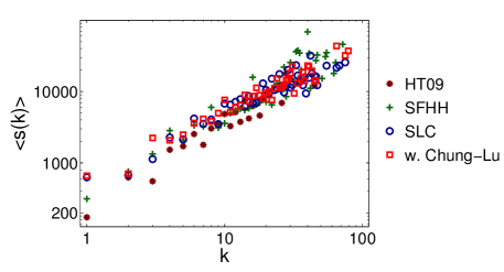
Figure 3: (Color online) Average strength versus degree of nodes in three different scientific conferences (described in Section C.2). The squares represent the same quantity for a weighted Chung-Lu graph generated from the empirical distributions of the SLC contact network.

B.2 Validation of the bootstrap test

A Monte-Carlo approach is used to validate the proposed method in the case of weighted Chung-Lu graphs. The goal is here to check the false alarm rate (rate at which normal groups are rejected) of the test. For this purpose, we generate $1000$ instances of weighted Chung-Lu graphs. The Null Hypothesis selected is “having the same modularity and the same cardinality” as $X^{0}$ as it is one of the most representative Hypothesis to assess a group’s behavior with respect to human social contacts. The described method is applied to $1000$ random sub-groups (one in each of the thousand generated weighted Chung-Lu graphs), with different significance levels $\alpha$ (from $1\%$ to $10\%$) and relaxation factors $\delta$ for the modularity constraint (from $0.03$ to $1.0$, with an additional case $\delta=\infty$ that corresponds to no constraint on modularity). In general, a random group in a weighted Chung-Lu graph should be classified as normal, and should not be rejected by the test. This is what we verify here.

Figure 4 shows the false alarm rate (i.e., the frequency of rejection of the Null Hypothesis) that is obtained in these simulations, divided by the prescribed significance level $\alpha$. For the test to be sound, this value has to always be bounded by $1$. This is indeed the case. Moreover, the value is often much lower than $1$ (between $0.3$ and $0.6$). This is a sign that the Bonferonni correction is pessimistic; it conducts us to reject more often the Null Hypothesis than we should when the group under study is drawn according to the Null Hypothesis. This is not an actual problem in the study as we are more interested in being certain that a group that is not rejected is indeed normal – and this is the case.

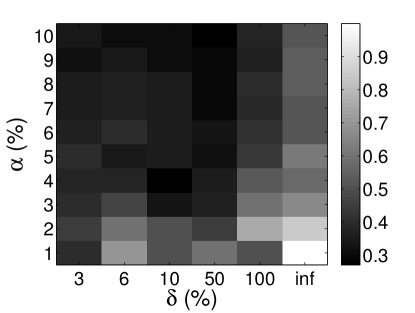
Figure 4: Ratio of the obtained false alarm rate (probability of rejecting the Null Hypothesis when it is true) divided by the maximum (pessimistic) significance level $\alpha$ of the test, in the case of the weighted Chung-Lu model, for the Null Hypothesis: “same cardinality and same modularity”. The prescribed significance level $\alpha$ acts as expected by the Bonferroni correction as a pessimistic bound to the true false alarm rate (hence, the ratio is always lower than 1). The results are displayed as function of $\alpha$ and $\delta$. It shows that the larger $\alpha$ is, the less tight the bound is. When $\delta$ increases, the obtained false alarm rate becomes closer to $\alpha$.

B.3 Controlling the size of the bootstrap space and the power of the test

In order to derive thresholds $\delta^{*}$ and maximal values $\chi^{2*}$ and $\sigma_{u}^{*}$ for each given constraint, we take a different perspective and use a notion of rarity: when a value is in the bulk of a distribution it is considered as common enough and when it is in the extreme tails, it is considered as too rare. To illustrate the argumentation, we focus on the constraint “same cardinality and same modularity”, where the strength of the “same modularity” constraint is tuned by $\delta$. Once more, we consider $1000$ weighted Chung-Lu graphs (computed with the empirical distributions of the data of Appendix C), and, within each Chung-Lu graph, $10000$ random groups of cardinal $M=39$ (one of the group sizes studied later on). Figure 5 shows the histogram of the modularity for the partition of the graph in such a group and its complementary. Typical groups give a small modularity, the mode of the histogram being between $-0.03$ and $0.03$. We define as rare groups those whose modularity are in the extreme tails of the distribution: either larger than its $10^{6}$ upper quantile or smaller than its $10^{6}$ lower quantile (these quantiles are reasonably estimated as we have $10^{7}$ samples in the distribution). The choice of these particular quantiles is somehow arbitrary but it can be easily changed for the following study and does not influence the general approach. This gives us two modularity boundaries $Q_{l}^{*}=-0.050$ and $Q_{u}^{*}=0.076$ that separate common enough groups (having modularities in the bulk of the distribution) from rare groups.

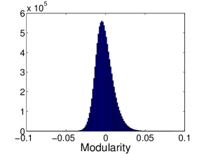
Figure 5: Histogram of the modularity of a sub-graph of $39$ nodes in a weighted Chung-Lu graph

We take the point of view that the test should indicate that the Null Hypothesis is true for all common groups (output number 2 in the list of Section II.5). Indeed, weighted Chung-Lu graphs are random and random groups in these graphs have in general no reason to be abnormal. Now, consider a group $X^{0}$ with modularity around $-0.005$ (the peak of the distribution). For a given $\delta$, the simulated annealing procedure will draw bootstraps from this distribution: there is a high chance that the bootstrap set’s modularities end up close to $-0.005$. Hence $X^{0}$ is compared to very similar groups even for high $\delta$: the test will always output $d=0,\chi^{2}<\chi^{2*},\sigma_{u}<\sigma_{u}^{*}$ (apart maybe for extremely small $\delta$). But as one approaches the modularity boundaries $Q^{*}$, the test will start to misclassify $X^{0}$ as abnormal for a large enough $\delta$. Indeed, consider a group with a modularity close to or equal to one of the boundaries (for instance $Q_{u}^{*}$). For a too large $\delta$, the bootstrap set’s modularities will still tend towards the small modularities that have a higher chance to be picked, and the test will be rejected. If we want all common groups with high modularity to be classified as normal, we need to have small enough $\delta$: this defines a first bound $\delta_{u}$ for $\delta$: $\delta<\delta_{u}$. The same argumentation holds for common groups with low modularity (close to $Q_{l}^{*}$), giving another bound $\delta_{l}$ for $\delta$: $\delta<\delta_{l}$. Overall, we thus obtain an upper bound for $\delta^{*}$: $\mbox{min}(\delta_{l},\delta_{u})$. In order to decide where in the range $[0,\mbox{min}(\delta_{l},\delta_{u})]$ we should choose $\delta^{*}$, the trade-off discussion of Section II.5 between precision of the Null Hypothesis and power of the test still holds. We give priority to the power of the test and choose the maximum possible value of $\delta$, equal to the upper bound: $\delta^{*}=\mbox{min}(\delta_{l},\delta_{u})$. In practice, as shown in Table 4, $\delta^{*}$ is between $5\%$ and $15\%$: the Null Hypotheses are still reasonably precise.

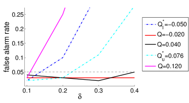
Figure 6: (Color online) False alarm rate as function of $\delta$ for groups of 39 nodes of varying modularities (describing the rarity of the groups) in weighted Chung-Lu graphs. Groups with modularity $Q$ outside the interval $([Q_{l}^{*}=-0.05,Q_{u}^{*}=0.076])$ are rare, and the others are considered common enough. To keep the false alarm rate under the expected significance level $\alpha$ (here equal to $5\%$ and represented by the horizontal dashed line) for all common groups, maximum values $\delta_{l}^{*}=0.15$ and $\delta_{u}^{*}=0.20$ are read on the plot. This in turn gives a general threshold $\delta^{*}=\mbox{min}(\delta_{l}^{*},\delta_{u}^{*})=0.15$.

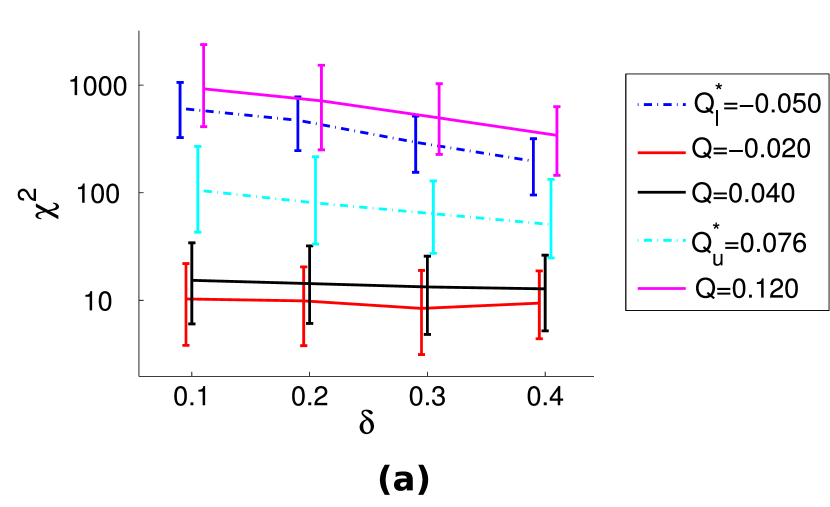
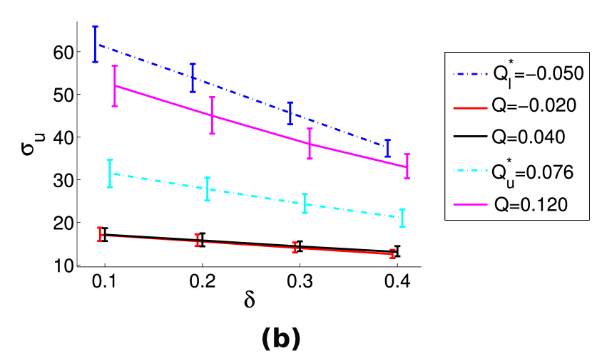
Figure 7: (Color online) $\chi^{2}$ (a) and $\sigma_{u}$ (b) as a function of $\delta$ for groups of varying modularities (describing the rarity of the groups) in weighted Chung-Lu graphs. As the test is designed to be valid for all common enough groups (i.e., with modularity $Q\in[Q_{l}^{*}=-0.05,Q_{u}^{*}=0.076]$) if one uses $\delta^{*}=0.15$, the maximum values $\sigma_{u}^{*}$ and $\chi^{2*}$ that should be accepted for $\sigma_{u}$ and $\chi^{2}$ are read from the curves. This procedure gives roughly $\chi^{2*}=950$ and $\sigma_{u}^{*}=60$.

Figure 6 shows the false alarm rate obtained in simulations for weighted Chung-Lu graphs as a function of $\delta$ for groups of 39 nodes of varying modularities (both common and rare). As expected, for very common groups (like groups with $Q=0.02$), the false alarm rate is constant with respect to $\delta$. On the contrary, the more we consider groups close to the boundaries $Q_{l}^{*}$ and $Q_{u}^{*}$, the faster the rate increases with $\delta$. The simulations were conducted on 100 different Chung-Lu graphs. To keep the false alarm rate under the expected significance level $\alpha$ (here equal to $5\%$) for all common groups, a maximum value $\delta^{*}$ for $\delta$ is obtained from this Figure. For the lower quantile $Q_{l}^{*}$ one reads $\delta_{l}=0.15$ and for the upper quantile $Q_{u}^{*}$ we obtain $\delta_{u}=0.20$. The general bound for the modularity constraint for groups of $39$ nodes is then $\delta^{*}=\mbox{min}(\delta_{l},\delta_{u})=0.15$. In fact, if one chooses $\delta<\delta^{*}$, all normal common groups will be correctly classified (with a tolerance of $\alpha=5\%$).

The next step is to find thresholds in the acceptable values for $\sigma_{u}$ and $\chi^{2}$. On Figure 7, these indicators are displayed as a function of $\delta$ for groups of $39$ nodes of varying modularities. As expected, $\chi^{2}$ and $\sigma_{u}$ increase monotonically with the rarity of the considered groups (for a fixed value of $\delta$). As we argued that the test is designed to classify all common groups as normal if one uses $\delta=\delta^{*}$, the maximum values $\sigma_{u}^{*}$ and $\chi^{2*}$ that have to be tolerated for $\sigma_{u}$ and $\chi^{2}$ are read from the curves as the maximum expected values for these common groups (we use the quantile at $95\%$ to fix a reasonable maximum value). One reads the approximate values $\chi^{2*}(\delta^{*};Q=Q_{l}^{*})=950$, $\sigma_{u}^{*}(\delta^{*};Q=Q_{l}^{*})=60$ and $\chi^{2*}(\delta^{*};Q=Q_{u}^{*})=250$, $\sigma_{u}^{*}(\delta^{*};Q=Q_{u}^{*})=30$. The general thresholds are therefore: $\chi^{2*}=\mbox{max}(\chi^{2*}(\delta^{*};Q=Q_{l}^{*}),\chi^{2*}(\delta^{*};Q=Q_{u}^{*}))=950$ and $\sigma_{u}^{*}=\mbox{max}(\sigma_{u}^{*}(\delta^{*};Q=Q_{l}^{*}),\sigma_{u}^{*}(\delta^{*};Q=Q_{u}^{*}))=60$.

The final conclusion of this validation procedure is that, once one has decided upon $\alpha$, a type of constraint, the cardinality of groups of interest, and a criterion to decide what common enough (i.e., not too rare) means for groups, it is possible to quantify the bootstrap approach presented here and to propose a value $\delta^{*}$ and thresholds $\sigma_{u}^{*}$ and $\chi^{2*}$. We show $(\delta^{*},\sigma_{u}^{*},\chi^{2*})$ for all the different constraints and all the different cardinalities used in Section III in Table 4-a. In Appendix C and Section III, we will compare the output of the test for four different groups with different Null Hypotheses. To be able to compare properly, we will use a unique value of $\delta^{*}$ for each Null Hypothesis. Therefore, out of the four $\delta^{*}$ proposed (one for each cardinality), we keep the minimum one and obtain the equivalent $\sigma_{u}^{*}$ and $\chi^{2*}$ for each cardinality. We sum up these values in Table 4-b.

For the study presented in this paper, we have therefore used these values of $\delta^{*}$, $\chi^{2*}$ and $\sigma_{u}^{*}$ obtained with the weighted Chung-Lu graphs used as surrogates of social networks.

Null Hypothesis	$M=39$	$M=73$	$M=99$	$M=106$
$Q_{X}$ constraint	$(0.15,950,60)$	$(0.15,110,45)$	$(0.15,40,35)$	$(0.15,40,30)$
$N_{XX}$ constraint	$(0.15,3500,85)$	$(0.05,2700,115)$	$(0.05,2600,125)$	$(0.05,2200,125)$
$T_{XX}$ constraint	$(0.15,3600,80)$	$(0.1,2200,100)$	$(0.05,3700,135)$	$(0.05,2700,135)$

a)

Null Hypothesis	$M=39$	$M=73$	$M=99$	$M=106$
$Q_{X}$ constraint with $\delta^{*}=0.15$	$(950,60)$	$(110,45)$	$(40,35)$	$(40,30)$
$N_{XX}$ constraint with $\delta^{*}=0.05$	$(5200,95)$	$(2700,115)$	$(2600,125)$	$(2200,125)$
$T_{XX}$ constraint with $\delta^{*}=0.05$	$(4300,90)$	$(3700,120)$	$(3700,135)$	$(2700,135)$

b)

Table 4: a) $(\delta^{*},\sigma_{u}^{*},\chi^{2*})$ for different constraints and cardinalities. $(\delta^{*},\sigma_{u}^{*},\chi^{2*})$ for the $Q_{X}$ constraint and $M=39$ are read from Figures 6 and 7 as explained in the text. Figures used to obtain the values for other constraints and other cardinalities are not shown. b) For each constraint, we decide to keep a unique $\delta^{*}$: the minimum of the four $\delta^{*}$ (one for each cardinality). We show here the corresponding $(\sigma_{u}^{*},\chi^{2*})$ for all cardinalities.

Appendix C Presentation of the Dataset of Two Co-located conferences

C.1 Data and pre-processing

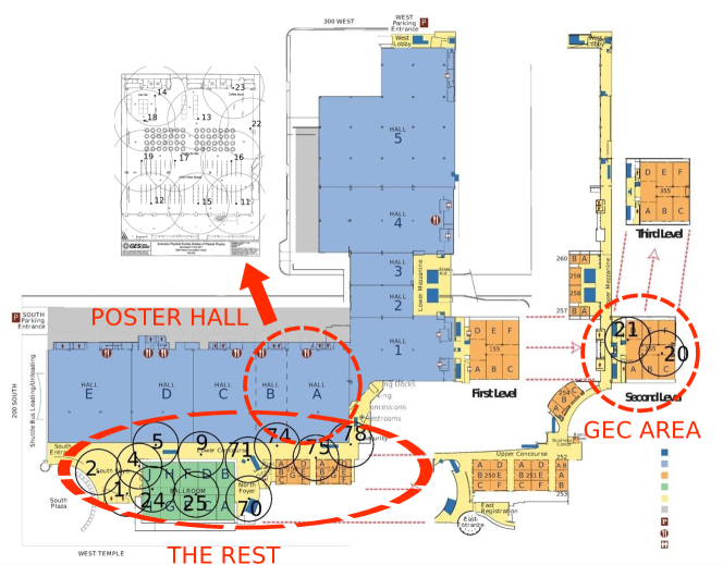
Figure 8: General map of the conference venue with the three different general areas. Each black circle corresponds to one of the 25 RFID readers used to measure the social interactions. The GEC area is isolated: it is 500 meters away from the Poster Hall.

The data was collected in Salt Lake City (SLC) in November 2011 during two co-located scientific conferences lasting five days, using the SocioPatterns sensing infrastructure www.sociopatterns.org ; Cattuto et al. (2010) to measure face-to-face proximity of individuals. The conferences were jointly organised by the DPP (Division of Plasma Physics) of the American Physical Society and the GEC (Gaseous Electronics Conference). Figure 8 shows the map of the conference venue in Salt Lake City.

Out of the 2081 participants of the conference, 320 agreed to participate in our study: 281 from DPP and 39 from GEC. The participation was on a voluntary basis so that there was no specific sampling scheme. The face-to-face proximity of the participants was measured using the SocioPatterns sensing infrastructure www.sociopatterns.org ; Cattuto et al. (2010) based on unobstrusive active RFID tags that can be embedded in conference badges. Two tags exchange radio packets only if the individuals wearing them face each other (the human body acts as a shield at the frequency and power of the radio packets) within a distance of 1 to 1.5 meters. The detected proximity relations are reported by the tags to RFID readers installed in the environment. At the end of the conference, the raw data consists of a log of all the recorded contacts. The log is a sequence of lines $(t,r,i,j)$ where $t$ is the time at which reader $r$ received the information that the individuals wearing tags $i$ and $j$ were in close face-to-face proximity (“in contact”). Given the operating parameters of the tags, proximity of two individuals wearing the RFID badges can be assessed with a probability in excess of $99\%$ over an interval of $20$ seconds Cattuto et al. (2010), which is a fine enough time scale to resolve human mobility and proximity at social gatherings. We therefore aggregate the raw data over time windows of $20$ seconds: we partition the five days of data gathering into $20$ second periods, and we associate to each of these periods $t$ the adjacency matrix $A^{t}$ representing the aggregated graph over the 20 seconds: $A_{ij}^{t}=1$ if and only if vertices $i$ and $j$ have exchanged at least one radio packet during the time window $t$, otherwise $A_{ij}^{t}=0$.

Overall, the data define a temporal contact network in which nodes represent individuals, and a link between two nodes at time $t$ denotes the fact that the corresponding individuals are in face-to-face proximity. The temporal network can moreover be aggregated over the total duration of the conference, defining a weighted contact network where each node is an individual and where the weight of a link between two individuals gives the cumulated time they have spent in face-to-face interaction during the conference.

C.2 Distributions of contact durations

We first compare briefly the gathered data with other datasets collected in similar contexts using the same infrastructure. We define a contact between two tags $i$ and $j$ as an unbroken subsequence of $1$’s within the sequence $\{A_{ij}^{t}\}$. Its duration is the length of this subsequence. Table 5 presents basic statistics of the present data, together with the ones collected during the 2009 ACM HyperText conference (HT09) Isella et al. (2011) and during a congress of the Société Française d’Hygiène Hospitalière (SFHH) Cattuto et al. (2010). Note that the sum of the total number of contacts (and the total time of contact) within DPP and within GEC does not exactly account for the interactions for the conference taken as a whole (ALL), due to the interactions between DPP and GEC. The SLC data contain a relatively small number of contacts, in comparison with the other conferences, taking into account the number of participants and the duration: this is due to the small sampling rate of the total population of the SLC conferences. Figure 9 however shows that various statistical properties of the contact networks, such as the distribution of the duration of contacts, the distribution of degrees, of the inter-contact times or of the weights of the links, are however very similar in the three contexts. This confirms the robustness of the main statistical properties of the networks of face-to-face contacts between individuals observed in previous works Isella et al. (2011); Eagle and Pentland (2006); Hui et al. (2005).

	HTT09	SFHH	SLC
			GEC	DPP	ALL
No. of tags	113	418	39	281	320
sample rate	75%	33%	12%	16%	15%
No. of days	2	2	5
No. of contacts	9582	27434	1189	21519	23920
Tot. time of contact (hours)	102	414	18	306	339

Table 5: Basic statistics concerning the datasets collected in three different scientific conferences.

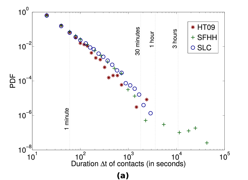
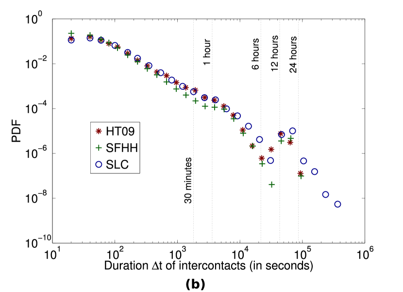
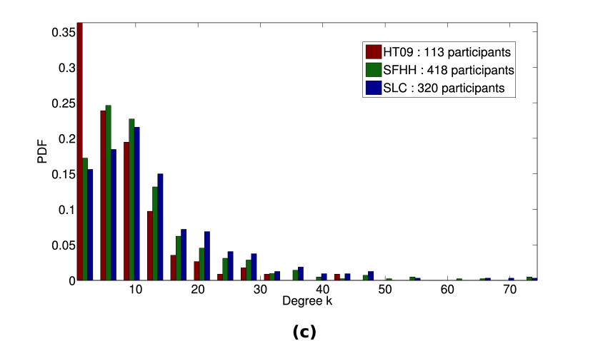
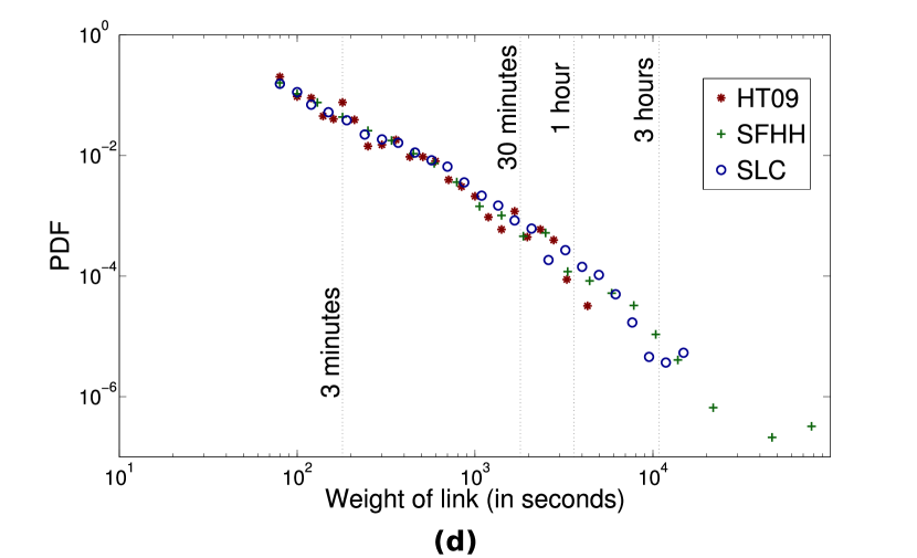
Figure 9: (Color online) (a) Comparison of the distribution of the durations of contacts for three different datasets. (b) Distribution of the duration of intercontact times. An intercontact interval is defined as the interval, for each node, between the starting times of two successive contacts. (c) Distribution of the degrees in the aggregated network of the three conferences. The degree of a participant corresponds to the total number of participants with whom s/he has been in contact during the conference. (d) Distribution of link weights. The weight of a link between two nodes gives the total time in contact of the corresponding participants.

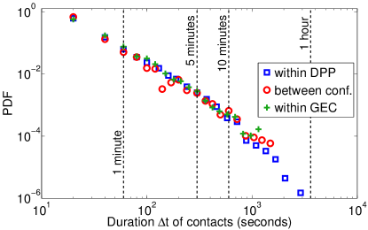
Figure 10: (Color online) Cumulative distributions of the durations of contacts within the DPP conference, within the GEC conference and between both conferences of the SLC dataset.

In the present dataset, we can distinguish three categories of contacts: within DPP, within GEC, and between both groups. Figure 10 shows that even though the number of contacts is much larger within DPP than within GEC (see Table 5), the corresponding duration distributions collapse remarkably well upon one another. Hence, we do not observe any difference in the statistical behavior of the three categories of contacts. Let us also note that we are not interested here in modeling these distributions (for instance by power law or log-normal functional forms), as the method we will use is data-driven. It is however of interest to remark that the broad shape of the distributions implies that parametric statistical methods would be hard to implement, and that data-driven statistical methods are expected to be more adequate.

C.3 Distributions of the durations of contacts taking place in different areas

The conference venue is spatially heterogeneous, with in particular three broadly defined areas: the GEC Area where the GEC registration and coffee breaks took place; the Poster Hall, where the poster sessions of both conferences took place; and the Rest, which includes the DPP registration desk, two coffee break areas, and corridors linking different parts of the building. The GEC Area was situated $500$ meters from the Poster Hall (maps are shown in Annex B). It therefore took time and energy to walk from one area to another, which was an obstacle to interactions between both groups. As the measuring infrastructure allows us to identify the area in which each reported contact took place, it is interesting to investigate if differences exist between the three types of contacts defined above when the spatial information is taken into account.

To this aim, we show in Fig. 11 the histograms of contact durations broken down by category of contact and area. For the DPP contacts (left panel), the distributions measured in the various areas have similar shapes, and the differences come from the overall number of contacts measured in each area (as members of the DPP did not go much to the GEC area). On the other hand, for the contacts between both groups (middle panel) and for the GEC contacts (right panel), different slopes are observed depending on the area of interest. Broader distributions are obtained in the Poster Hall, in particular for the contacts between GEC and DPP attendees: the Poster Hall was therefore a more favorable setting for long cross-group contacts. This leads us to a somehow obvious remark: organizing activities in common physical spaces favors the mixing between two groups.

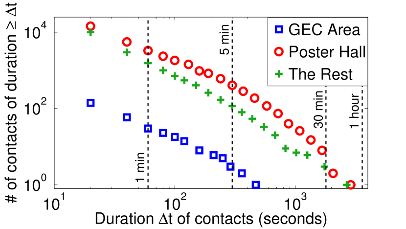
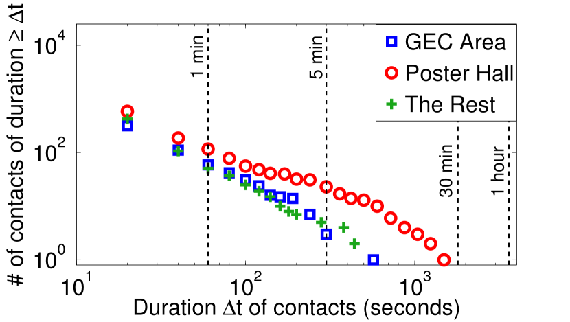
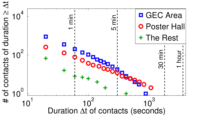
Figure 11: (Color online) Cumulative histograms of the durations of contacts in the three different areas within the SLC conference. Results for: (left) contacts within the DPP members, (middle) contacts between both conferences and (right) contacts within the GEC members.

Appendix D Co-located conferences case study: Cardinality constraint

We describe here the results of the test using only the cardinality constraint to test if the GEC group behaves normally. We thus consider the following simple Null Hypothesis: GEC behaves like any random group of $M=39$ individuals in the conference. For this first Null Hypothesis, the only constraint we impose to the bootstrap samples is therefore to have a cardinality equal to $M$.

Applying the protocol described in II.2, we first pick randomly with replacement $N_{B}=1000$ bootstraps samples of $39$ nodes. For each sample, we compute the seven associated observables and normalize them as proposed in II.3. For each observable $Z$, the empirical distribution function $\hat{D}_{z}^{b}$ are computed from the bootstrap samples: the $1-\alpha^{\prime}$ two-sided acceptance interval for $\hat{D}_{z}^{b}$ defines what we call the “normal behavior” of a group under this constraint. We then obtain the divergences $d_{z}$ for each feature, and finally the triplet $(d,\chi^{2},\sigma_{u})$.

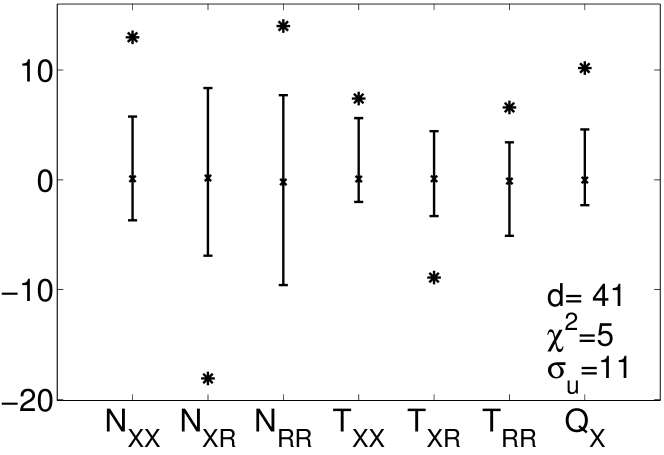
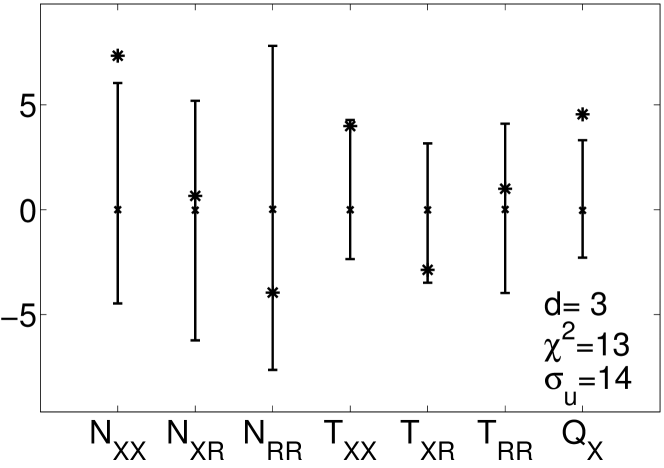
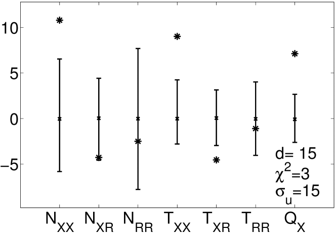
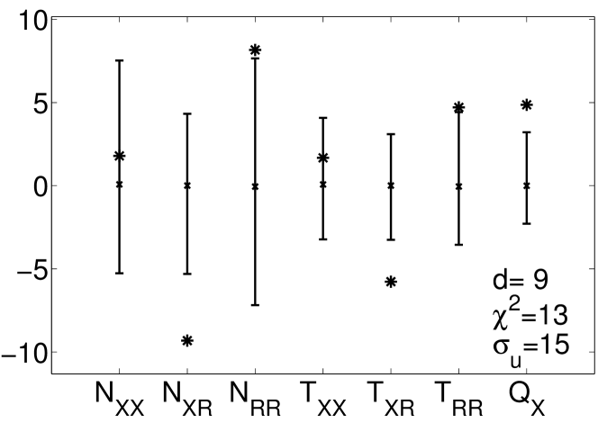
Figure 12: Results of the test with same cardinality constraint for the four groups: GEC (top left), STP (top right), JUP (bottom left), and SEP (bottom right). For each $z$, the two-sided acceptance interval with $1-\alpha^{\prime}$ significance level are in black and the value $z^{0}$ is the black star. Here, $\alpha=5\%$, i.e. $\alpha^{\prime}=\frac{\alpha}{F-f}=\frac{0.05}{7}=0.7\%$. For each group $X^{0}=$ GEC, STP, JUP and SEP, the scalar $d$ (bottom right hand corner of each figure) is the total divergence between the acceptance interval of the bootstrap samples and the real data. $\chi^{2}$ and $\sigma_{u}$ are the two control parameters of the size of the bootstrap space.

The top left plot of Figure 12 summarizes the output of this test for GEC: for each feature, the two-sided acceptance interval with $1-\alpha^{\prime}$ significance level is shown by a black line (its median being the black cross) for the $\hat{D}_{z}^{b}$ of the bootstrap samples, and the measured value of $z^{0}$ for GEC is figured by black stars. Finally, the values of $d$, $\chi^{2}$ and $\sigma_{u}$ are reported in the bottom right hand corner of the plot. Figure 1a displays the two histograms yielding the two indicators $\sigma_{u}$ and $\chi^{2}$ in this case of cardinality constraint for $X^{0}$=GEC: they are both small. The other three plots of Figure 12 show the corresponding results for the three other groups (SEP, JUP, STP).

The indicators $\chi^{2}$ and $\sigma_{u}$ are small enough for the four groups, indicating that the bootstrap sets are large enough and that the test is fair according to the chosen Null Hypothesis, as commented in Section II.5 and Appendix B.3. For all four groups, $d$ is non-null and the Null Hypothesis is rejected. In other words, none of these groups of individuals behaves similarly to a random group of nodes with the same cardinality. These results do not come as a surprise since, as previously mentioned, these groups are somehow expected to behave as communities and behave indeed as such: compared to the bootstrap samples, they tend to have larger $Q_{X}$, $N_{XX}$, $N_{RR}$, $T_{XX}$, $T_{RR}$ and smaller $N_{XR}$, $T_{XR}$. Interestingly, GEC’s divergence is clearly larger than the others: this first test, even if somehow naïve, hints at some difference between GEC and the other groups.