Material Dependence of the Wire-Particle Casimir Interaction

Abstract

We study the Casimir interaction between a metallic cylindrical wire and a metallic spherical particle by employing the scattering formalism. At large separations, we derive the asymptotic form of the interaction. In addition, we find the interaction between a metallic wire and an isotropic atom, both in the non-retarded and retarded limits. We identify the conditions under which the asymptotic Casimir interaction does not depend on the material properties of the metallic wire and the particle. Moreover, we compute the exact Casimir interaction between the particle and the wire numerically. We show that there is a complete agreement between the numerics and the asymptotic energies at large separations. For short separations, our numerical results show good agreement with the proximity force approximation.

I Introduction

Casimir forces contribute significantly to the effective interaction of micro- and nanometer sized structures Dalvit et al. (2011). For identical objects or mirror symmetric configurations, this type of interaction is attractive Kenneth and Klich (2006) and can cause stiction in micro-motors and other similar structures Serry et al. (1998). More generally, if the permittivities of the objects are higher or lower than those of the surrounding medium, any equilibrium position of the objects is unstable due to the Casimir interactions Rahi et al. (2010). Therefore, a good quantitative understanding of such forces is a key parameter in the design and manufacturing of micro-mechanical devices.

It is important to study the Casimir forces for different shapes as they strongly depend on the geometry and material properties Kardar and Golestanian (1999); U. Mohideen and Mostepanenko (2009); Dalvit et al. (2011). Technically, investigating the interplay between the shape and material effects is quite involved. The scattering formalism provides a powerful tool to calculate the Casimir interaction between objects of general shape and material properties Rahi et al. (2009). There is much recent research activity based on the scattering formalism, e.g., for edges and tips Maghrebi et al. (2011); Graham et al. (2010), anisotropic particles Emig et al. (2009), wires and plates Noruzifar et al. (2011, 2012); Emig et al. (2006); Rahi et al. (2008), and spheres and plates Zandi et al. (2010).

An important geometry which has not yet been investigated in detail, consists of a wire and a particle (atomic or macroscopic). In the plane-particle geometry this force is known as Casimir-Polder (CP) interaction Casimir and Polder (1948). Our study of the wire-particle case is motivated by theories Arnecke et al. (2008) and experiments Denschlag et al. (1998); Bawin and Coon (2001) on the two-dimensional quantum scattering of neutral atoms or molecules at wires or nanotubes. In an early work, the interaction between a filament and an isotropic atom has been studied for perfectly and non-perfectly conducting metals Barash and Kyasov (1989). Later, Eberlein and Zietal studied the interaction between a neutral atom and a perfect metal cylinder, using perturbation theory Eberlein and Zietal (2007, 2009). Recently, the Casimir energy for a polarizable micro-particle and an ideal metal cylindrical shell has been computed using the Green’s function technique Bezerra et al. (2011). The focus of previous studies were mainly on the interaction between a metal wire and a perfect metal particle or an atom. Therefore, the influence of material properties of the spherical particles on the energy remains to be studied in detail.

In this work, we study the Casimir interaction between a metallic spherical particle and cylindrical metallic wire where the latter is described by the Drude, plasma or perfect metal model. Using the scattering formalism, we derive a general expression for the Casimir interaction between the particle and cylinder. From this general expression we determine the behavior of the Casimir energy in various limiting cases (separation regimes) analytically, and numerically over a wide range of separations. Interestingly, we find ranges of distances in which the Casimir interaction does not depend on the material properties of the metallic wire. In contrast, we find that the interaction depends in general on the material properties of the metallic particle at all separations. An exception is the plasma sphere with a plasma wavelength that is much smaller than the size of the sphere for which the Casimir interaction is universal at asymptotically large distances. At short separations, we compute the exact Casimir interaction numerically and compare it both with the asymptotic results and the prediction of proximity force approximation (PFA). In both limits we obtain good agreement.

The structure of the rest of the paper is as follows: In Sec. II, we review the scattering approach and derive the elements that are needed for computing the interaction between a wire and a particle. In Sec. III, the large–distance asymptotic interaction between a metallic wire and a particle (metal sphere and isotropic atom) is derived for the perfect metal, plasma and Drude models. In Sec. IV, the exact Casimir interaction is computed numerically and compared with the asymptotics expansions. Section V is dedicated to the interaction at short separations where the PFA is expected to become reliable.

II Method

We consider a cylindrical wire separated by a distance $d$ from a spherical particle. We use the scattering formalism to calculate the Casimir energy between the cylinder and sphere Rahi et al. (2009). In general, the Casimir free energy between two objects at the temperature $T$ is given by

$${\mathcal{E}}=k_{B}T{{\sum_{n=0}^{\infty}}^{\prime}}\ln\,{\det}\left[{\bf 1}-\mathbb{N}(\kappa_{n})\right]\,,$$ (1)

where $\bf 1$ is the identity matrix, $\kappa_{n}$ is the Matsubara wave number $\kappa_{n}=2\pi nk_{B}T/\hbar c$ and the matrix $\mathbb{N}$ factorizes into the scattering amplitudes (T-matrices) as well as translation matrices which describe the coupling between the multipoles on distinct objects. The primed sum denotes that the contribution of $n=0$ has to be weighted by a factor of $1/2$.

At zero temperature, the primed sum in Eq. (1) is replaced by an integral along the imaginary frequency axis,

$${\mathcal{E}}=\frac{\hbar c}{2\pi}\int_{0}^{\infty}d\kappa\ln\det\left({\bf 1}-\mathbb{N}\right)\,,$$ (2)

with $\kappa$ the Wick-rotated frequency. The elements of the matrix $\mathbb{N}$ for electric ($E$) and magnetic ($M$) polarizations ($\alpha,~{}\beta,~{}\gamma=E,~{}M$) and cylindrical wave functions $m$ and $m^{\prime}$ are

$${\mathbb{N}}_{k_{z}m,k_{z}^{\prime}m^{\prime}}^{\alpha\beta}=\sum_{\gamma=E,M}\sum_{{m^{\prime\prime}}=-\infty}^{\infty}T_{{\rm s},k_{z}m,k_{z}^{\prime}m^{\prime\prime}}^{\alpha\gamma}\,\\ \times\sum_{n=-\infty}^{\infty}{\mathcal{U}}^{\rm sc}_{k_{z}^{\prime}m^{\prime\prime}n}\,T_{{\rm c},k_{z}^{\prime}n}^{\gamma\beta}\,{\mathcal{U}}^{\rm cs}_{{k_{z}^{\prime}}nm^{\prime}}\,,$$ (3)

where $k_{z}$ is the wave number along the $z$-axis$,T_{\rm c}$ and $T_{\rm s}$ are the T-matrices of the cylinder and sphere in cylindrical basis, respectively. The translation matrix $\mathcal{U}^{\rm sc}$ relates regular cylindrical vector waves to outgoing ones.

The translation matrices do not couple different polarizations and for both $E$ and $M$ polarizations, their matrix elements are given by

$${{\mathcal{U}}^{\rm sc}_{nn^{\prime}}} =(-1)^{n^{\prime}}\,K_{n-n^{\prime}}(p\,d)\,,$$

$${\mathcal{U}}^{\rm cs}_{nn^{\prime}} =(-1)^{n-n^{\prime}}{\mathcal{U}}^{\rm sc}_{nn^{\prime}}\,,$$ (4)

where $p=\sqrt{\kappa^{2}+k_{z}^{2}}$ and $K_{n}(x)$ is the modified Bessel function of the second kind. Note that the $\mathbb{N}$-matrix elements in Eq. (3) are written in cylindrical basis to avoid the complicated form of the translation matrices in the spherical basis Rahi et al. (2009).

The T-matrix of the sphere in cylindrical basis is derived in Appendix B and is given by

$$T_{{\rm s},k_{z}m,k_{z}^{\prime}m}^{{\alpha\gamma}}=\frac{1}{2\pi\kappa L}\sum_{\ell={\rm max}(1,|m|)}^{\infty}\sum_{{\beta}}(1-2\delta_{{\alpha,\beta}})$$

$$\times D^{\dagger}_{k_{z}m{\alpha},\ell m{\beta}}\,T_{{\rm s},\ell m}^{{\beta}}\,D_{\ell m{\beta},k_{z}^{\prime}m{\gamma}}\,,$$ (5)

where $L$ is the length of the cylinder, $\ell$ is the quantum number of the spherical electromagnetic waves, ${\beta}=E,~{}M$ is the electromagnetic polarization and $D$ is the conversion matrix from the cylindrical to spherical basis. The elements of the conversion matrix are given in Appendix C . Note that in Eq. (II), $T_{\rm s,\ell m}^{{\beta}}$ is the T-matrix of the sphere in the spherical basis.

To obtain the Casimir energy from Eq. (2), we plug Eqs. (II) and (II) into (3) and use the identity $\det({\bf 1}-{\bf AB})=\det({\bf 1}-{\bf BA})$. The $\mathbb{N}$-matrix for the energy between the sphere and the cylinder is rewritten as

$${\mathbb{N}}_{\ell m,\ell^{\prime}m^{\prime}}^{{\alpha\beta}}=\frac{1}{4\pi^{2}\kappa}\sum_{{\gamma,\gamma^{\prime}}}T_{{\rm s},\ell m}^{{\alpha}}\int_{-\infty}^{\infty}dk_{z}\,{D}_{\ell m{\alpha},k_{z}m{\gamma}}\,\,\\ \times{\bf\tilde{T}}_{mm^{\prime}}^{{\gamma\gamma^{\prime}}}{D}^{\dagger}_{k_{z}m^{\prime}{\gamma^{\prime}},\ell^{\prime}m^{\prime}{\beta}}(1-2\delta_{{\beta,\gamma^{\prime}}})\,,$$ (6)

with

$${\bf\tilde{T}}_{mm^{\prime}}^{{\gamma\gamma^{\prime}}}=\sum_{n=-\infty}^{\infty}{\mathcal{U}}_{k_{z}mn{\gamma}}^{\rm cs}\,T^{{\gamma\gamma^{\prime}}}_{{\rm c},k_{z}n}\,{\mathcal{U}}_{k_{z}nm^{\prime}{\gamma^{\prime}}}^{\rm sc}\,.$$ (7)

In this work, to study the impact of the material properties of the metallic objects on the Casimir interaction, we employ the plasma, Drude and perfect metal dielectric properties with the constant magnetic permeability $\mu=1$. The Drude model dielectric response is given by

$$\epsilon(ic\kappa,\lambda_{\rm p},\lambda_{\sigma})=1+\frac{(2\pi)^{2}}{(\lambda_{\rm p}\kappa)^{2}+\lambda_{\sigma}\kappa/2}\,,$$ (8)

where $\lambda_{\rm p}$ is the plasma wave length and $\lambda_{\sigma}=2\pi c/\sigma$ is the length scale associated with the conductivity $\sigma$. Equation (8), reproduces the plasma model dielectric function for $\lambda_{\sigma}=0$. Note that the material properties of the sphere and the cylinder enter to the calculations through the T-matrices, see Appendix A.

III Large-separation regime: asymptotic Casimir energy

In this section, we study the large separation asymptotic behavior of the Casimir interaction between a particle and a wire. We consider a spherical particle with radius $R_{\rm s}$ and a cylindrical wire with radius $R_{\rm c}$. In order to find the large–distance ($d\gg R_{\rm c},R_{\rm s}$) asymptotic form of the Casimir interaction, one has to find the behavior of the T-matrices in the low-frequency limit.

III.1 Asymptotic Behavior of T-matrices

III.1.1 T-matrix of a wire

In this part, we obtain the asymptotic form of the T-matrix elements of a wire at large separations. Using the dielectric function given in Eq. (8), we find the T-matrix element of the wire for $E$ polarization and $n=0$ at small frequencies ($\kappa\ll 1,~{}k_{z}/\kappa~{}{\rm fixed}$) is

$$T^{EE}_{0}\approx-\frac{p^{2}}{C(\kappa)-p^{2}\ln(pR_{\rm c})}\,,$$ (9)

where $p=\sqrt{\kappa^{2}+k_{z}^{2}}$. The parameter $C(\kappa)$ depends on the dielectric properties of the wire. For a perfect metal wire $C(\kappa)=0$ and for a plasma wire with the plasma wavelength $\lambda_{\rm p}$, $C(\kappa)\approx\lambda_{\rm p}^{2}\kappa^{2}/(2\pi^{2}R_{\rm c}^{2})$ if the plasmon oscillations cannot build up transverse to the wire axis as the diameter is too small, i.e., $R_{\rm c}\ll\lambda_{\rm p}$. In the opposite limit we approximately reproduce the T-matrix of a perfect metal wire, i.e. $C(\kappa)\approx 0$. For a Drude wire with the conductivity $\sigma$ and the characteristic length $\lambda_{\sigma}$, $C(\kappa)=\lambda_{\sigma}\kappa/(4\pi^{2}R_{\rm c}^{2})$ if $\kappa\ll\lambda_{\sigma}/\lambda_{\rm p}^{2},1/\lambda_{\sigma}$. The first condition ($\kappa\ll\lambda_{\sigma}/\lambda_{\rm p}^{2}$) means that the Drude behavior dominates over the plasma behavior, equivalent to the fact that in the dominator of Eq. (8), the first term is much smaller than the second one. The second condition ($\kappa\ll 1/\lambda_{\sigma}$) ensures that the Drude dielectric function is much larger than one, i.e., the metallic behavior is dominant Noruzifar et al. (2011, 2012).
At large separations, $T^{EE}_{0}$ elements dominate over the other T-matrix elements since $T^{EM}_{0}=T^{ME}_{0}=0$, $T^{MM}_{0}\sim\kappa^{2}$, and for $n\neq 0$ partial waves $T_{n}\sim\kappa^{2|n|}$. Note that for Drude cylinders $T^{EE}_{0}\sim\kappa$ while for plasma and perfect metal cylinders $T^{EE}_{0}\sim 1$.

III.1.2 T-matrix of a particle

The T-matrix elements of a spherical particle have a different scaling compared to the ones for the cylindrical wire. For the plasma and perfect metal spheres $T_{{\rm s},\ell m}\sim\kappa^{2\ell+1}$. For Drude spheres the T-matrix elements for the electric $E$ and magnetic $M$ polarizations scale differently: $T^{M}_{{\rm s},\ell m}\sim\kappa^{2(\ell+1)}$ and $T^{E}_{{\rm s},\ell m}\sim\kappa^{2\ell+1}$. Therefore, the asymptotic behavior of the T-matrix at large separations is dominated by the $\ell=1$ elements. The asymptotic form of the T-matrix elements for the magnetic polarization $M$ and $\ell=1$ depends on the material properties of the sphere. While for a perfect metal sphere, we have

$$T_{{\rm s},1m}^{M}\approx-\kappa^{3}R_{\rm s}^{3}/3\,,$$ (10)

for a plasma sphere with the plasma wavelength $\lambda^{\prime}_{\rm p}$, we obtain

$$T_{{\rm s},1m}^{M}\approx-\frac{1}{3}\frac{I_{5\over 2}(2\pi R_{\rm s}/\lambda^{\prime}_{\rm p})}{I_{1\over 2}(2\pi R_{\rm s}/\lambda^{\prime}_{\rm p})}\kappa^{3}R_{\rm s}^{3}\,.$$ (11)

Note that in the limit of perfect conductivity $\lambda_{\rm p}^{\prime}\to 0$, we reproduce Eq. (10).

For a Drude sphere with the conductivity $\sigma^{\prime}$ and the characteristic length $\lambda^{\prime}_{\sigma}$,

$$T_{{\rm s},1m}^{M}\approx-\frac{8\pi^{2}}{45}\frac{R_{\rm s}}{\lambda^{\prime}_{\sigma}}\kappa^{4}R_{\rm s}^{4}\,.$$ (12)

However, the asymptotic form of the T-matrix elements for $E$ polarization and $\ell=1$, up to the leading order, does not depend on the material properties, and is the same for the perfect metal, plasma and Drude models,

$$T_{{\rm s},1m}^{E}\approx\frac{2}{3}\kappa^{3}R_{\rm s}^{3}\,.$$ (13)

Note that for the Drude sphere $T_{{\rm s},1m}^{M}\sim\kappa^{4}$, and thus we add the sub-leading term to the expansion of $T_{{\rm s},1m}^{E}$ in Eq. (13) and obtain

$$T_{{\rm s},1m}^{E}\approx\frac{2}{3}\kappa^{3}R_{\rm s}^{3}-\frac{1}{4\pi^{2}}\frac{\lambda_{\sigma}^{\prime}}{R_{\rm s}}\kappa^{4}R_{\rm s}^{4}\,,$$ (14)

where the sub-leading term contains the material properties of the Drude wire.

III.1.3 T-matrix of an Atom

The above approach can also be used to calculate the Casimir energy between an atom and a wire. To this end, we consider a neutral two-level atom in the ground state, with the transition frequency $\omega_{10}$ Casimir and Polder (1948). We assume that the distance from the atom to the wire $d$ is much larger than the radius of the wire $R_{\rm c}$, i.e. $d/R_{\rm c}\gg 1$. Moreover, we assume that the atom is isotropic and does not have magnetic polarizability. In the isotropic-dipole approximation, the only nonzero element of the T-matrix reads

$$T^{E}_{{\rm atom},1m}\approx\frac{2}{3}\alpha^{E}(\kappa)\,{\kappa^{3}}\,,$$ (15)

where $\alpha^{E}$, the electric polarizability, is given by

$$\alpha^{E}(\kappa)=\frac{\alpha_{0}}{1+\kappa^{2}d_{10}^{2}}\,,$$ (16)

with $d_{10}=c/\omega_{10}$, $\alpha_{0}=f_{10}e^{2}/(m\omega_{10}^{2})$, $e$ the electron charge, $m$ the mass and $f_{10}$ the oscillator strength of the $0\rightarrow 1$ transition.

III.2 Asymptotic Energy Expression

In this subsection, using the asymptotic T-matrix expressions and Eq. (6), we derive the Casimir energy at large separations. Considering ${\ln{\rm det}\equiv{\rm Tr}\ln}$, we expand the integrand in Eq. (2) in powers of $\mathbb{N}$ for $\kappa\ll 1$ and $k_{z}/\kappa$ fixed and find

$${\mathcal{E}}\approx-\frac{\hbar c}{2\pi}\int_{0}^{\infty}d\kappa\,{\rm Tr}{{\mathbb{N}}}\,.$$ (17)

As discussed above, in the limit $d\gg R_{\rm s},R_{\rm c}$ only the $\ell=1$ terms contributes to the sphere T-matrix, $T_{{\rm s},\ell m}$. Therefore, only the partial wave numbers $m=0,\pm 1$ have to be taken into account to obtain the matrix ${\mathbb{N}}$. Using Eq. (6), we find

$${\rm Tr}\,{\mathbb{N}}\approx\sum_{\gamma}\sum_{m=-1}^{1}\tilde{\mathbb{N}}_{1m,1m}^{{\gamma\gamma}}\\ =\frac{1}{4\pi^{2}\kappa}\sum_{{\gamma}}\sum_{m=-1}^{1}T_{{\rm s},1m}^{{\gamma}}\int_{-\infty}^{\infty}dk_{z}\,{\tilde{D}}_{1m{\gamma},k_{z}mE}\,{\bf\tilde{T}}_{m{m}}^{EE}\,\\ \times{\tilde{D}}^{\rm T}_{k_{z}mE,1m{\gamma}}(1-2\delta_{{\gamma},E})\,,$$ (18)

with $\tilde{\bf D}$ the modified conversion matrix with real elements. The modified conversion matrix is related to the original one by ${\bf D}_{\ell m,k_{z}m}=(-1)^{\ell-m}(-i)^{\ell+m-1}{\tilde{\bf D}}_{\ell m,k_{z}m}$ , see Appendix C. Furthermore, the matrix ${\bf\tilde{T}}_{mm}^{EE}$ in Eq. (18) is equal to

$${\bf\tilde{T}}_{mm}^{EE}\approx K_{m}^{2}(pd)T^{EE}_{{\rm c},k_{z}0}\,.$$ (19)

Note that in Eq. (19), $T^{EE}_{{\rm c},k_{z}\pm 1}$ are neglected as they scale with higher powers of $\kappa$.

Inserting Eq.(19) into Eq. (18) and performing the sums, we find

$$-{\rm Tr}[\tilde{\mathbb{N}}]\approx\frac{1}{4\pi^{2}\kappa}\int_{-\infty}^{\infty}dk_{z}\,T^{EE}_{{\rm c},k_{z}0}\\ \times\left[K_{0}^{2}(pd)({\tilde{D}}_{10E,k_{z}0M}^{2}T^{M}_{{\rm s},1}-{\tilde{D}}_{10M,k_{z}0M}^{2}T^{E}_{{\rm s},1})\right.\\ \left.+2K_{1}^{2}(pd)({\tilde{D}}_{11E,k_{z}1M}^{2}T^{M}_{{\rm s},1}-{\tilde{D}}_{11M,k_{z}1M}^{2}T^{E}_{{\rm s},1})\right]\,.$$ (20)

The modified conversion matrix elements in Eq. (20) are (see Appendix C for all details ),

$${\tilde{D}}_{10E,k_{z}0M} = 0,~{}~{}~{}~{}~{}~{}{\tilde{D}}_{10M,k_{z}0M}=\sqrt{6\pi}(1+k_{z}^{2}/k^{2})^{1/2},$$

$${\tilde{D}}_{11E,k_{z}1M} = \sqrt{3\pi},~{}~{}{\tilde{D}}_{11M,k_{z}1M}=\sqrt{3\pi}k_{z}/k.$$ (21)

Inserting Eq. (III.2) into Eq. (20) and using the leading term in the $T^{E}_{{\rm s},1m}$ expansion, we find the asymptotic energy between a perfect metal, plasma and Drude cylinder and a spherical particle or an atom. Using Eq. (17) and the T-matrix expansions up to $\kappa^{3}$, see Eqs. (10)-(14), we obtain the general expression for the asymptotic energy

$$\frac{\mathcal{E}}{\hbar c}\approx\frac{1}{\pi^{2}}\int_{0}^{\infty}d\kappa\int_{0}^{\infty}dk_{z}\,T^{EE}_{{\rm c},0}\\ \times\chi\left(p^{2}K_{0}^{2}(pd)+(2\Lambda_{0}\kappa^{2}+k_{z}^{2})K_{1}^{2}(pd)\right)\,,$$ (22)

with $\chi=R_{\rm s}^{3}$ for the spherical particle and $\chi=\alpha^{E}(\kappa)$ for the isotropic atom. Moreover, $\Lambda_{0}$ is proportional to $T^{M}_{{\rm s},1}$, see Eq. (20), with $\Lambda_{0}=1/4$ for the perfect metal particle, $\Lambda_{0}={I_{5\over 2}(2\pi R_{\rm s}/\lambda^{\prime}_{\rm p})}/({4I_{1\over 2}(2\pi R_{\rm s}/\lambda^{\prime}_{\rm p})})$ for the plasma particle and $\Lambda_{0}=0$ for the atom and the Drude particle. The latter is due to the fact that $T^{M}_{{\rm s},1}$ is set to zero in Eq. (22). $T^{M}_{{\rm s},1}$ for the atom is indeed zero and for the Drude particle scales with $\kappa^{4}$, see Eq. (12). Therefore, for the Drude particle the asymptotic energy given by Eq. (22) needs a correction because of the $\kappa^{4}$ terms in Eqs. (12) and (14), which is

$$\frac{\delta{\mathcal{E}}_{\rm DS}}{\hbar c}=\frac{1}{\pi^{2}}\int_{0}^{\infty}\kappa\,d\kappa\int_{0}^{\infty}dk_{z}\,T^{EE}_{{\rm c},0}\\ \times\chi\left(\frac{3\lambda_{\sigma}^{\prime}}{8\pi^{2}}p^{2}K_{0}^{2}(pd)+\left[\frac{3\lambda_{\sigma}^{\prime}}{8\pi^{2}}k_{z}^{2}-\frac{4\pi^{2}R_{s}^{2}}{15\lambda_{\sigma}^{\prime}}\kappa^{2}\right]K_{1}^{2}(pd)\right)\,.$$ (23)

Inserting Eq. (9) into Eq. (22) and using the polar coordinates, $\kappa\to\rho\cos(\theta)/d$ and $k_{z}\to\rho\sin(\theta)/d$, we find

$$\frac{\mathcal{E}}{\hbar c}\approx-\frac{1}{\pi^{2}d^{4}\ln(2d/R_{\rm c})}\int_{0}^{\infty}d\rho\rho^{3}\int_{0}^{\pi/2}\frac{d\theta}{1+C(\rho,\theta)}\\ \times\chi\left(K_{0}^{2}(\rho)+(\sin^{2}(\theta)+2\Lambda_{0}\cos^{2}(\theta))K_{1}^{2}(\rho)\right)\,,$$ (24)

where for the perfect metal cylinder $C(\rho,\theta)=0$, for the plasma cylinder $C(\rho,\theta)\approx\xi\cos^{2}(\theta)$ with $\xi={{\lambda_{\rm p}^{2}}/(2\pi^{2}R_{\rm c}^{2}}\ln(2d/R_{\rm c}))$, and for the Drude cylinder $C(\rho,\theta)=\xi^{\prime}\cos(\theta)/\rho$ with $\xi^{\prime}=\lambda_{\sigma}d/(4\pi^{2}R_{\rm c}^{2}\ln(2d/R_{\rm c}))$.

The correction $\delta{\mathcal{E}}_{\rm DS}$ for the Drude particle in polar coordinates $(\rho,\theta)$ reads

$$\frac{\delta{\mathcal{E}}_{\rm DS}}{\hbar c}=\frac{3R_{\rm s}^{3}\,\lambda_{\sigma}^{\prime}}{8\pi^{4}d^{5}\ln(2d/R_{\rm c})}\int_{0}^{\infty}\rho^{4}\,d\rho\int_{0}^{\pi/2}d\theta\,\frac{\cos(\theta)}{1+C(\rho,\theta)}\\ \times\left(K_{0}^{2}(\rho)+\left[\sin^{2}(\theta)-\frac{32\pi^{4}R_{s}^{2}}{45\lambda_{\sigma}^{\prime 2}}\cos^{2}(\theta)\right]K_{1}^{2}(\rho)\right)\,.$$ (25)

Now we use Eqs. (24) and (25) for different material properties and calculate the Casimir interaction for various limiting cases.

III.3 The Casimir interaction between a wire and a spherical particle

Below we present the large separation asymptotic energies between a metallic spherical particle and a metallic wire.

III.3.1 The perfect metal wire

For a perfect metal wire and a perfect metal, plasma or Drude particle, the energy integral in Eq. (24) results into

$$\frac{\mathcal{E}}{\hbar c}\approx-\frac{\Lambda_{0}+1}{3\pi}\frac{R_{\text{s}}^{3}}{d^{4}\ln(2d/R_{\rm c})}\,.$$ (26)

It is important to note that Eq. (26) depends on the material properties of the spherical particle through the quantity $\Lambda_{0}$. For a perfect metal wire and a plasma particle, in the limiting case of small plasma wavelengths, ${\lambda^{\prime}}_{\rm p}\ll R_{\rm s}$, we reproduce the perfect conductivity form with ${{\Lambda}_{0}}\approx 1/4$. In the limit of large plasma wavelengths, ${\lambda^{\prime}}_{\rm p}\gg R_{\rm s}$, we obtain $\Lambda_{0}\approx{\pi^{2}R_{\rm s}^{2}}/{(15{\lambda^{\prime}}_{\rm p}^{2})}$. Since $\Lambda_{0}\ll 1$, the plasma wavelength of the spherical particle does not have a significant contribution to the asymptotic energy.

For the Drude particle, using Eq. (25), the correction to the asymptotic energy given by Eq. (26) reads

$$\frac{\delta{\mathcal{E}}_{\rm DS}}{\hbar c}=-\frac{R_{\rm s}^{3}}{32\,d^{5}\,\ln(2d/R_{\rm c})}\left(\frac{\pi^{2}R_{\rm s}^{2}}{2\,\lambda_{\sigma}^{\prime}}-\frac{63\,\lambda_{\sigma}^{\prime}}{64\,\pi^{2}}\right)\,,$$ (27)

and scales with $d^{-5}$. Depending on the terms in the brackets, this correction can have a significant contribution to the asymptotic energy. In the limit of high conductivity, $\lambda_{\sigma}^{\prime}\ll R_{\rm s}$, the first term in the brackets dominates over the second one. For this specific case, if $\lambda_{\sigma}^{\prime}d\ll R_{\rm s}^{2}$ the correction becomes even larger than the asymptotic energy itself, i.e. $\delta{\mathcal{E}}_{\rm DS}\gg{\mathcal{E}}$.

Note that in Eq. (27), the second term in the brackets dominates only at low conductivity limit $\lambda_{\sigma}^{\prime}\gg R_{\rm s}$ in which the spherical particle is considered to be a very poor conductor. In general, the second term does not have a noticeable contribution to the asymptotic energy for good conductors such as copper and gold.

III.3.2 The plasma wire

For a plasma wire and a plasma or a perfect metal particle, the polar and radial integrals in Eq. (24) can easily be performed,

$$\frac{\mathcal{E}}{\hbar c}\approx-\frac{R_{\text{s}}^{3}}{\pi d^{4}\ln(2d/R_{\rm c})}f(\xi)\,,$$ (28)

with

$$f(\xi)=\frac{1}{3\xi}(2\Lambda_{0}-1)\left(1-(1+\xi)^{-{1\over 2}}\right)+\frac{1}{2}(1+\xi)^{-{1\over 2}}\,,$$ (29)

where $\xi$ is given below Eq. (24), $\xi=\lambda_{\rm p}^{2}/(2\pi^{2}R_{\rm c}^{2}\ln(2d/R_{\rm c}))$. In the small plasma wavelength limit, $\lambda_{\rm p}/R_{\rm c}\ll\sqrt{\ln(2d/R_{\rm c})}$, we reproduce the perfect metal wire results given by Eqs. (26) and  (27).

In the opposite limit $\lambda_{\rm p}/R_{\rm c}\gg\sqrt{\ln(2d/R_{\rm c})}$, the asymptotic energy reads

$$\frac{\mathcal{E}}{\hbar c}\approx-\frac{R_{\rm c}R_{\text{s}}^{3}}{\lambda_{\rm p}d^{4}}\left(\frac{1}{\sqrt{2\ln(2d/R_{\rm c})}}+\frac{4\pi\Lambda_{0}}{3}\frac{R_{\rm c}}{\lambda_{\rm p}}\right)\,,$$ (30)

For a perfect metal spherical particle, $\Lambda_{0}=1/4$, and the second term can be neglected as we are at the large plasma wavelength regime.

For a plasma spherical particle with plasma wavelength $\lambda_{\rm p}^{\prime}$, if $\lambda_{\rm p}^{\prime}\ll R_{\rm s}$, $\Lambda_{0}\approx 1/4$ and the energy is the same as in the case of a perfect particle and a plasma wire. In the opposite limit $\lambda_{\rm p}^{\prime}\gg R_{\rm s}$, we have $\Lambda_{0}\approx{\pi^{2}R_{\rm s}^{2}}/{(15{\lambda^{\prime}}_{\rm p}^{2})\ll 1}$ and the plasma wavelength of the particle does not have a significant effect on the asymptotic energy, and the asymptotic energy is mainly dominated by the material properties of the plasma wire.

For a Drude particle, the asymptotic energy is given by Eq. (30) together with a correction obtained by Eq. (25). The correction reads

$$\frac{\delta{\mathcal{E}}_{\rm DS}}{\hbar c}=-\frac{3}{64}\frac{R_{\rm s}^{3}}{d^{5}}\left(\frac{R_{\rm c}}{\lambda_{\rm p}}\right)^{2}\left(\frac{9}{4}(\frac{5}{8}-\ln 2)\lambda_{\sigma}^{\prime}+\pi^{4}\frac{R_{\rm s}^{2}}{\lambda_{\sigma}^{\prime}}\right)\,.$$ (31)

Since for good conductors $\lambda_{\sigma}^{\prime}\ll R_{\rm s}$, similar to the case of a perfect metal wire, the second term dominates over the first one.

III.3.3 The Drude wire

For a Drude wire and a perfect metal or plasma particle, in the limit $\xi^{\prime}\ll 1$ or $d^{2}/R_{\rm c}^{2}\ll d/\lambda_{\sigma}$, using Eqs. (24) and (25), we reproduce the perfect metal wire results, see Eqs. (26) and (27).

In the opposite limit, $\xi^{\prime}\gg 1$ or equivalently $d^{2}/R_{\rm c}^{2}\gg d/\lambda_{\sigma}$ and $d\gg\lambda_{\rm p}^{2}/\lambda_{\sigma}$ the integrations in Eq. (24) result into

$$\frac{\mathcal{E}}{\hbar c}\approx-\frac{9\pi^{2}}{64}\frac{R_{\text{s}}^{3}R_{\rm c}^{2}}{\lambda_{\sigma}d^{5}}\left(5\Lambda_{0}+4\ln({\lambda_{\sigma}d}/{R_{\rm c}^{2}})\right)\,.$$ (32)

For a perfect metal particle, $\Lambda_{0}=1/4$, and the energy given by Eq. (32) is always attractive since $\lambda_{\sigma}d\gg R_{\rm c}^{2}$.

For the plasma particle, in the limit of small plasma wavelengtha $\lambda_{\rm p}^{\prime}\ll R_{\rm s}$, $\Lambda_{0}\approx 1$ and the particle behaves like a perfect metal. In the opposite limit, $\lambda_{\rm p}^{\prime}\gg R_{\rm s}$, as previously seen, we find $\Lambda_{0}\approx{\pi^{2}R_{\rm s}^{2}}/{(15{\lambda^{\prime}}_{\rm p}^{2})}$. In this case the second term in Eq. (32) dominates, which means that the material properties of the plamsa particle does not have a significant effect on the asymptotic Casimir energy.

Under the same condition $\xi^{\prime}\gg 1$, using Eq. (25), the correction to Eq. (32) reads

$$\frac{\delta{\mathcal{E}}_{\rm DS}}{\hbar c}=-\frac{R_{\rm c}^{2}\,R_{\rm s}^{3}\ln(2d/R_{\rm c})}{\lambda_{\sigma}d^{6}}\left(\frac{32\pi^{3}R_{\rm s}^{2}}{25\lambda_{\sigma}^{\prime}}-\frac{7\lambda_{\sigma}^{\prime}}{5\pi}\right)\,.$$ (33)

As discussed above, for metallic particles, the second term in Eq. (33) is much smaller than the first one.

III.4 The Casimir energy between a wire and an Atom

We calculate the Casimir energy between a wire and an atom in both retarded and non-retarded limits. To find the asymptotic energies at large separations, we use Eq. (24) with $\Lambda_{0}=0$:

III.4.1 The retarded limit

In the retarded limit, $d\gg d_{10}$, we find the Casimir energy between a perfect metal wire and an atom as

$$\frac{\mathcal{E}}{\hbar c}\approx-\frac{1}{3\pi}\frac{\alpha_{0}}{d^{4}\ln(2d/R_{\text{c}})}\,.$$ (34)

Equation (34) is in complete agreement with the results in Refs. Eberlein and Zietal (2007, 2009); Bezerra et al. (2011); Barash and Kyasov (1989). It is important to note that even though the asymptotic energies for an atoms given in Eq. (34) and for a perfect metal particle given in Eq. (26) have the same scaling behavior, the numerical coefficients do not match; $1/(3\pi)$ for the atom and $5/(12\pi)$ for the spherical particle. This discrepancy is due to the lack of magnetic polarizability in the isotropic atoms.

For the plasma wire and an atom in the limit $\xi\gg 1$ or equivalently $\lambda_{\text{p}}/R_{\text{c}}\gg\sqrt{\ln(2d/R_{\text{c}})}$ and $d\gg d_{10}$, the asymptotic energy reads

$$\frac{\mathcal{E}}{\hbar c}\approx-\frac{R_{\text{c}}}{\lambda_{\text{p}}}\frac{\alpha_{0}}{d^{4}\sqrt{2\ln(2d/R_{\text{c}})}}\,,$$ (35)

which is in agreement with the atom–plasma wire result in Ref. Barash and Kyasov (1989). In the limit $\lambda_{\text{p}}/R_{\text{c}}\ll\sqrt{\ln(2d/R_{\text{c}})}$ and $d\gg d_{10}$, we reproduce the perfect metal wire-atom interactin energy given in Eq. (34).

For the Drude wire and an atom, in the region of intermediate distances $\xi^{\prime}\gg 1$ or equivalently $d/R_{\rm c}\gg R_{\rm c}/\lambda_{\sigma}$, in the retarded limit $d\gg d_{10}$, the asymptotic energy reads

$$\frac{\mathcal{E}}{\hbar c}\approx-\frac{9\pi^{2}}{16}\frac{\alpha_{0}R_{\rm c}^{2}}{\lambda_{\sigma}d^{5}}\ln({\lambda_{\sigma}d}/{R_{\rm c}^{2}})\,.$$ (36)

Equation (36) is in agreement with Ref. Barash and Kyasov (1989). In the opposite limit, $\xi^{\prime}\ll 1$ or $d/R_{\rm c}\ll R_{\rm c}/\lambda_{\sigma}$ and $d\gg d_{10}$, once again we reproduce the perfect metal wire-atom asymptotic interaction energy, see Eq. (34).

III.4.2 The non-retarded limit

In the non-retarded limit, $d\ll d_{10}$, using Eq. (24) with $\Lambda_{0}=0$, we perform the angular integral for the perfect metal, plasma and Drude wires.

For the perfect metal wire, the radial integral can easily be obtained. Expanding the result of the integral for $d\ll d_{10}$ yields

$$\frac{\mathcal{E}}{\hbar}\approx-\frac{\pi}{16}\frac{\alpha_{0}\,\omega_{10}}{d^{3}\,\ln(2d/R_{\text{c}})}\,.$$ (37)

For the plasma wire, the radial integral over $\rho$ in Eq. (24) cannot readily be performed in the non-retarded limit. Therefore, we expand the integrand for $d/d_{10}\ll 1$. In the limit $d\ll R_{\text{c}}d_{10}/\lambda_{\text{p}}$ the expansion of the integrand does not depend on the material properties up to the leading order. Therefore, performing the integration over $\rho$ results into the perfect metal wire-atom interaction energy given in Eq. (37).

Similar to the plasma wire, the radial integration in Eq. (24) is not easily calculable for the Drude wire. Analogously, we expand the integrand for $d/d_{10}\ll 1$ and then perform the integral over $\rho$. In the limit $d\ll R_{\text{c}}\sqrt{d_{10}/\lambda_{\sigma}}$, we find Eq. (37) for a perfect metal wire and an atom. This is due to the fact that the material properties of the Drude wires does not play any role ate intermediate separations, see Refs. Noruzifar et al. (2012, 2011).

III.5 Universality

In previous sections, we have derived the asymptotic energies between a metallic wire and a metallic spherical particle for different dielectric properties, described by the Drude, plasma or perfect metal models. We have found that in all cases, the Casimir energy depends on the material properties of the spherical particle. This is due to the fact that the material property of a sphere has a significant contribution to its T-matrix Zandi et al. (2010).

In contrast, for parallel metallic wires and a wire–plate geometry, at intermediate distances, the asymptotic energy does not depend on the material properties of the objects and is universal Noruzifar et al. (2011, 2012).

Although in a wire–sphere system the Casimir interaction depends on the material properties of the particle at all separations, the signatures of the universal behavior of the metallic wire is still traceable at asymptotic separations. For a plasma wire at intermediate distances, $d/R_{\rm c}\ll\exp(\lambda_{\rm p}^{2}/R_{\rm c}^{2})$, the Casimir interaction depends both on the material properties of the wire and the particle. For larger separations, $d/R_{\rm c}\gg\exp(\lambda_{\rm p}^{2}/R_{\rm c}^{2})$, the interaction is independent of the material properties of the plasma wire, while it still depends on the material properties of the particle, see Fig.1a.

For a Drude wire and a metallic particle, at larger separations, $d^{2}/R_{\rm c}^{2}\gg d/\lambda_{\sigma}$, the interaction depends both on the material properties of the Drude wire and that of the spherical particle, see Fig.1b. At intermediate distances $d^{2}/R_{\rm c}^{2}\ll d/\lambda_{\sigma}$, while material properties of the sphere has a significant role in the Casimir energy, it does not depend on the material properties of the wire. Note that the casimir interaction is also independent of the material properties for two parallel Drude wires Noruzifar et al. (2011, 2012).

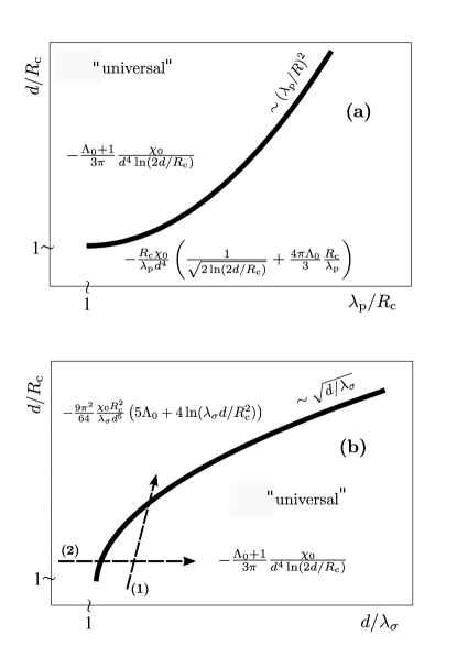
Figure 1: Interaction between a wire and a particle and between a wire and an atom in the retarded limit. The formulas describe the rescaled interaction energies, ${\cal E}/(\hbar c)$. The parameter $\chi_{0}=\alpha_{0}$ for the atom and $\chi_{0}=R_{\text{s}}^{3}$ for the particle. (a) Interaction between a plasma wire and a metallic spherical particle. The asymptotic results corresponds to the regimes sufficiently far from the curve $\ln(d/R_{\rm c})\sim(\lambda_{\rm p}/R_{\rm c})^{2}$ and for $d/R_{\rm c}$, $\lambda_{\rm p}/R_{\rm c}\gg 1$. (b) Interaction between a Drude wire and a metallic particle. The separating curve is given, up to logarithmic corrections, by $d/R_{\rm c}\sim\sqrt{d/\lambda_{\sigma}}$. The energy expressions hold for $d/R_{\rm c}$, $d/\lambda_{\sigma}\gg 1$ and $d\gg\lambda_{\rm p}^{2}/\lambda_{\sigma}$. Different regimes can be reached depending on the relative size of length scales: Arrow (1) corresponds to an increasing distance $d$ which ultimately leads to a strictly non-universal interaction. Arrow (2) indicates an overall increase of the geometry (i.e., $d/R_{\rm c}$ fixed) with constant conductivity leading to a “ universal ” interaction.

IV Intermediate-separation regime: numerical calculations

We use Eq. (2), to numerically calculate the Casimir energy. The numerical algorithm consists of three major parts: (i) constructing the matrix ${{\mathbb{N}}}$ from Eq. (6), (ii) computing the determinant of ${\bf 1}-{{\mathbb{N}}}$ for specific imaginary frequencies $\kappa$ and (iii) integrating over $\kappa$. The matrix ${\mathbb{N}}$ consists of blocks which are associated with the quantum numbers $\ell$ and $\ell^{\prime}$. We truncate $\ell$ and $\ell^{\prime}$ at a finite partial wave number $\ell_{\rm max}$ such that the result for the energy changes by less than a factor of $1.0001$ upon increasing $\ell_{\rm max}$ by $1$. Since $\ell,\ell^{\prime}\leq\ell_{\rm max}$, the N-matrix has $\ell_{\rm max}^{2}$ blocks $N_{\ell\ell^{\prime}}$. The block ${{\bf N}}_{\ell\ell^{\prime}}$ consists of the elements ${{\bf N}}_{\ell m,\ell^{\prime}m^{\prime}}$ which form $2\times 2$ blocks, with $m=-\ell,\dots,\ell$ and $m^{\prime}=-\ell^{\prime},\dots,\ell^{\prime}$,

$${{\bf N}}_{\ell m,\ell^{\prime}m^{\prime}}=\begin{pmatrix}{{\mathbb{N}}}^{MM}_{\ell m,\ell^{\prime}m^{\prime}}&{{\mathbb{N}}}^{ME}_{\ell m,\ell^{\prime}m^{\prime}}\\ {{\mathbb{N}}}^{EM}_{\ell m,\ell^{\prime}m^{\prime}}&{{\mathbb{N}}}^{EE}_{\ell m,\ell^{\prime}m^{\prime}}\end{pmatrix}\,.$$

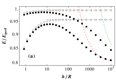
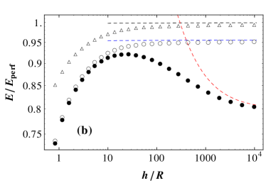
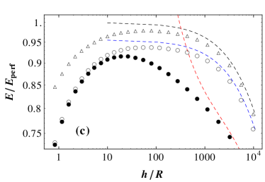
Figure 2: Ratio of the numerically computed energy $E$ for realistic metals to the perfect metal energy $E_{\rm perf}$ versus $h/R$ for a wire and a particle with $R_{\text{c}}=R_{\text{s}}=R$. Each figure shows the numerics related to a wire with specific material properties: (a) for a perfect metal wire; (b) a plasma wire with $\lambda_{\rm p}/R=0.5$ and (c) a Drude wire with the same value for $\lambda_{\rm p}/R$ and $\lambda_{\sigma}=\lambda_{\rm p}/27.4$. The ratio of energies for particles with different material properties are distinguished by different symbols: Open triangles for perfect metal particle and open circles and open squares for plasma particles with $\lambda_{\rm p}/R=0.5,~{}0.05$, respectively. Filled circles and filled squares denote Drude particles with $\lambda_{\rm p}/R=0.5,~{}0.05$, respectively, and $\lambda_{\sigma}=\lambda_{\rm p}/27.4$.

Consequently the size of the block ${{\bf N}}_{\ell\ell^{\prime}}$ is $(4\ell+2)\times(4\ell^{\prime}+2)$, implying that the off-diagonal blocks ($\ell\neq\ell^{\prime}$) are not square matrices. Furthermore, ${\mathbf{N}}_{\ell\ell^{\prime}}$ blocks are not diagonal since symmetry along the axis parallel to the wire’s axis is broken by the particle.

To construct the matrix ${{\mathbb{N}}}$, $4\ell^{2}_{\rm max}(\ell_{\rm max}+2)^{2}$ integrals over $k_{z}$ have to be evaluated for each $\kappa$. This makes the numerical computations for closer separations quite expensive. For example at separation $d/R=2.6$, the energy converges with $\ell_{\rm max}=12$, corresponding to a matrix of size $336$ with $112896$ $k_{z}$-integrals for just a single value of $\kappa$.

Figure 2 illustrates our numerical results for a metallic cylinder and a metallic spherical particle both with the radius $R$. The plots show the Casimir energy normalized to the energies for the perfect metal wire-particle configuration as a function of the surface-to-surface distance $h=d-2R$. For the numerical calculations, we used $\lambda_{\rm p}/R=0.05$ and $0.5$ with $\lambda_{\rm p}/\lambda_{\sigma}=27.4$, corresponding to the parameters for gold with $\lambda_{\rm p}=137$ nm and $\lambda_{\sigma}\approx 5$ nm Decca et al. (2007). Figure 2 shows the dependence of the Casimir energy on the material properties of the wire and particle. Figure 2(a) depicts the interaction energy between the perfect metal wire with the metallic particle for plasma (opensymbols) and Drude (filled symbols) models with $\lambda_{\rm p}/R=0.05$ (squares) and $0.5$ (circles) and $\lambda_{\rm p}/\lambda_{\sigma}=27.4$. The dashed lines show the asymptotic energies given by Eqs. (26) and (27). As shown in the figure, there is a very good agreement between the asymptotics and the numerical results. The numerical results confirm that at very large separations, only the material properties of the particle contribute to the Casimir energy. We note that in the range of distances considered here and for the parameters of gold, one has to consider the energy given in Eq. (26) in addition to the correction term presented in Eq. (27).

Figure 2(b) shows the interaction between a plasma wire and a perfect metal (open triangles), plasma (open circles) and Drude particles (filled circles) with the plasma wavelength $\lambda_{\rm p}/R=0.5$ and $\lambda_{\rm p}/\lambda_{\sigma}=27.4$. The dashed lines show the asymptotic energies given by Eqs. (30) and (31). This figure also shows the good agreement between the asymptotics derived in the previous section and our numerical results. Again, here it is important to include the correction given by Eq. (31). Note that for the perfect metal particle and the plasma cylinder (open triangles) the energy ratio approaches 1 at large separations. This is due to the fact that in this regime the material properties of the plasma wire do not contribute to the Casimir interaction, see Fig. 1(a).

Figure 2(c) shows the interaction between a Drude wire and a perfect metal (open triangles), a plasma (open circles) and a Drude spherical particles (filled circles) with $\lambda_{\rm p}/R=0.5$ and $\lambda_{\rm p}/\lambda_{\sigma}=27.4$. The dashed lines are obtained by computing the integrals in Eqs. (24) and (25). Since for $10^{2}\lesssim d\lesssim 10^{4}$ we have $10^{-2}\lesssim\xi^{\prime}\lesssim 10^{-1}$, corresponding to the crossover regime, the asymptotic energies of Eqs. (32) and (33) are not applicable, see Fig. 1(b).

V Short-separation regime: Proximity Force Approximation

In this section, using the Proximity Force Approximation (PFA) Derjaguin (1934), we calculate the Casimir interaction at short separations $h\ll R_{\rm c},R_{\rm s}$. This method gives the interaction as an integral of the energies between parallel surface segments,

$${\mathcal{E}}_{\rm PFA}=\int dA\,E_{\rm plate}(h)\,,$$ (38)

where $E_{\rm plate}$ is the Casimir energy per unit area between two parallel plates and $h$ is the surface-to-surface distance. Figure 3 illustrates the distance between two surface elements. According to Fig. 3 the distance $h$ is

Figure 3: The geometry of a wire of radius $R_{c}$ and a sphere of radius $R_{s}$ at a distance $h_{0}$ (center-to-center distance $d=h_{0}+R_{c}+R_{s}$).

$$h=h_{0}+R_{\rm s}(1-\cos(\theta_{\rm s}))+R_{\rm c}(1-\cos(\phi_{\rm c}))\,,$$ (39)

with $h_{0}=d-R_{\rm c}-R_{\rm s}$ the distance of the closest approach between the cylinder and the sphere. One can write $\phi_{\rm c}$ in terms of $\theta_{\rm s}$ and $\phi_{\rm s}$,

$$\sin(\phi_{\rm c})=\frac{R_{\rm s}}{R_{\rm c}}\sin(\theta_{\rm s})\sin(\phi_{\rm s})\,.$$ (40)

At short separations, the surface elements of the sphere and cylinder in which $\theta_{\rm s}\ll 1$ and $\phi_{\rm c}\ll 1$ respectively, contribute most to the interaction. Therefore, the distance $h$ can be approximated by

$$h(\theta_{\rm s},\phi_{\rm s})\approx h_{0}+\frac{R_{\rm s}\theta_{\rm s}^{2}}{2}(1+\frac{R_{\rm s}}{R_{\rm c}}\sin^{2}(\phi_{\rm s}))\,.$$ (41)

Inserting Eq. (41) into Eq. (38) and performing a simple change of variable, we obtain the PFA energy

$${\mathcal{E}}_{\rm PFA}=\frac{2\pi\,{R_{\rm s}}}{\sqrt{1+\frac{R_{\rm s}}{R_{\rm c}}}}\int_{h_{0}}^{\infty}d{H}\,E_{\rm plate}({H})\,.$$ (42)

For the case of perfect metal surfaces with $E_{\rm plate}(H)/A=-\pi^{2}\hbar c/(720H^{3})$, we find

$${\mathcal{E}}_{\rm PFA}=-\frac{\pi^{3}\,{R_{\rm s}}\,\hbar c}{720\sqrt{1+\frac{R_{\rm s}}{R_{\rm c}}}\,{h_{0}^{2}}}\,.$$ (43)

Figure 4: Ratio of the numerical results for the Casimir energy shown in Fig. 2 and the PFA energy for perfect metals (squares) and for plasma model with $\lambda_{p}/R=0.5$ (circles). The ratio is shown as a function of surface-to-surface distance $h$. Similar to Fig. 2, the wire and particle have equal radiuii $R_{\text{s}}=R_{\text{c}}=R$.

For Drude and plasma objects, we use the Lifshitz formula Lifshitz (1956),

$$\frac{{E}_{\rm plane}(h)}{A}=\frac{\hbar c}{(2\pi)^{2}}\int_{0}^{\infty}\kappa^{2}d\kappa\int_{1}^{\infty}p\,dp\\ \times\ln\left[(1-r^{M}_{\rm s}r^{M}_{\rm c}e^{-2\kappa ph})(1-r^{E}_{\rm s}r^{E}_{\rm c}e^{-2\kappa ph})\right]\,,$$ (44)

with $p$ a dimensionless variable, $r_{\rm s}^{{M(E)}}$ and $r_{\rm c}^{{M(E)}}$ the Fresnel coefficients of the surface elements for the cylinder and sphere, respectively. The Fresnel coefficients of an object $a$ are given by

$$r^{M}_{a}(ic\kappa,p) = \frac{\mu_{a}(ic\kappa)-\sqrt{1+(n_{a}^{2}(ic\kappa)-1)/p^{2}}}{\mu_{a}(ic\kappa)+\sqrt{1+(n_{a}^{2}(ic\kappa)-1)/p^{2}}}\,,$$

$$r^{E}_{a}(ic\kappa,p) = \frac{\epsilon_{a}(ic\kappa)-\sqrt{1+(n_{a}^{2}(ic\kappa)-1)/p^{2}}}{\epsilon_{a}(ic\kappa)+\sqrt{1+(n_{a}^{2}(ic\kappa)-1)/p^{2}}}\,,$$ (45)

where $n_{a}$ is the refraction index, $n_{a}(ic\kappa)=\sqrt{\epsilon(ic\kappa)\mu(ic\kappa)}$.

The PFA energy is obtained using Eqs. (42) and (44) together with the dielectric function of Eq. (8). Figure 4 shows the Casimir energy for a perfect metal (open squares) and plasma model $\lambda_{\rm p}/R=0.5$ (open circles) normalized to the PFA energy. The energies associated with the Drude model are not shown since they collapse on the data for the plasma model at short separations. Our data show that as the distance between the sphere and the cylinder decreases, the values of the energies become closer to the PFA ones. Note that at short separations the energy converges with larger values of $\ell_{\rm max}$. Since the size of the matrix $\tilde{\mathbb{N}}$ increases quadratically with $\ell_{\rm max}$ , the numerical calculation of the Casimir energy becomes extremely costly at short separations. In this work the interaction is calculated up to $h/R=0.4$.

VI Summary and Conclusions

In summary, we have studied the Casimir energy between a cylindrical wire and a spherical particle. For large separations, we have derived the asymptotic energies for the Drude, plasma and perfect metal models. In addition, we have calculated the Casimir interaction between a metallic wire and an isotropic atom. Our results for the wire–atom system is in complete agreement with previous results obtained through a different method Barash and Kyasov (1989); Eberlein and Zietal (2007, 2009); Bezerra et al. (2011) .

Furthermore, we have computed the Casimir interaction between a spherical particle and a wire. Such computations are quite demanding due to lack of spherical symmetry. Our numerical results perfectly match the asymptotic energies.

For short separations, we obtained the energy using the Proximity Force Approximation (PFA) and compared it with our numerical data. This comparison indicates that as the distance between the wire and particle decreases, the numerical results for the Casimir energy becomes closer to the PFA one. It is noteworthy that depending on the separation, the material properties of the metallic wire may not play a role in the interaction energy, similar to the parallel wires and wire–plate systems Noruzifar et al. (2011, 2012).

In a cylinder–sphere system, we do not observe a universal behavior as we have previously obtained for parallel wires and a wire–plate geometries because of the physical properties of the spherical particle. However, one can still have “universal” regimes in which the interaction does not depend on the material properties of the metallic wire.

In case of the plasma wire with the plasma wavelength $\lambda_{\rm p}$ and radius $R_{\rm c}$, at sufficiently large separations, $d/R_{\rm c}\gg\exp(\lambda_{\rm p}^{2}/R_{\rm c}^{2})$, the material properties of the wire does not play any role in the asymptotic interactions between the wire and a particle or an atom.
In contrast for the Drude wire with conductivity $\sigma$ and the characteristic length $\lambda_{\sigma}=2\pi c/\sigma$, at large separations $d^{2}/R_{\rm c}^{2}\gg d/\lambda_{\sigma}$, the asymptotic energy depends on the the material properties of the wire. Quite interestingly, in the opposite limit, $d^{2}/R_{\rm c}^{2}\ll d/\lambda_{\sigma}$ and $d\gg\lambda_{\rm p}^{2}/\lambda_{\sigma}$, the asymptotic interaction becomes independent of the material properties of the Drude wire. The specific behavior of the Drude wires has been explained in Refs. Noruzifar et al. (2011, 2012) in terms of large scale charge fluctuations.

At the end we emphasize that since simple generic geometries appear in many nano- and micrometer–sized systems, the knowledge of the interaction between a metallic sphere and cylinder could be important for an efficient design of low–dimensional structures.

Appendix A T-matrices

In this appendix, for completeness, we present the T-matrices of a cylinder and a sphere, from Refs. Noruzifar et al. (2011); Zandi et al. (2010).

The T-matrix of a sphere in spherical vector wave basis is diagonal in the quantum numbers $l$, $m$ and the electromagnetic polarizations $E$ and $M$

$$T^{\textsc{m}}_{s,\ell m}=-\frac{\pi}{2}\frac{\eta I_{l+{1\over 2}}(\kappa R)\left[I_{l+{1\over 2}}(n\kappa R)+2n\kappa RI^{\prime}_{l+{1\over 2}}(n\kappa R)\right]-nI_{l+{1\over 2}}(n\kappa R)\left[I_{l+{1\over 2}}(\kappa R)+2\kappa RI^{\prime}_{l+{1\over 2}}(\kappa R)\right]}{\eta K_{l+{1\over 2}}(\kappa R)\left[I_{l+{1\over 2}}(n\kappa R)+2n\kappa RI^{\prime}_{l+{1\over 2}}(n\kappa R)\right]-nI_{l+{1\over 2}}(n\kappa R)\left[K_{l+{1\over 2}}(\kappa R)+2\kappa RK^{\prime}_{l+{1\over 2}}(\kappa R)\right]}\,,$$ (46)

with $n=\sqrt{\epsilon(i\kappa)\mu(i\kappa)}$ and $\eta=\sqrt{\epsilon(i\kappa)/\mu(i\kappa)}$. The T-matrix elements for E-multipoles, $T^{\textsc{e}}_{s,\ell m}$, are obtained from Eq. (46) by interchanging $\epsilon$ and $\mu$.

The T-matrix elements of a cylinder with dielectric response $\epsilon(i\kappa)$ and magnetic permeability $\mu(i\kappa)$ are given by

$$T^{EE}_{k_{z}n} = -\frac{I_{n}(pR)}{K_{n}(pR)}\frac{\Delta_{2}\Delta_{3}+K^{2}}{\Delta_{1}\Delta_{2}+K^{2}}\,,$$ (47)

$$T^{EM}_{k_{z}n} = -\frac{K}{\sqrt{\epsilon\mu}(pR)^{2}K_{n}(pR)^{2}}\frac{1}{\Delta_{1}\Delta_{2}+K^{2}}\,,$$ (48)

with $K=({nk_{z}}/{(\sqrt{\epsilon\mu}R^{2}\kappa)})\left({1}/{p^{\prime 2}}-{1}/{p^{2}}\right)$ and

$$\Delta_{1} = \frac{I^{\prime}_{n}(p^{\prime}R)}{p^{\prime}RI_{n}(p^{\prime}R)}-\frac{1}{\epsilon}\frac{K^{\prime}_{n}(pR)}{pRK_{n}(pR)}\,.$$ (49)

Note that $\Delta_{2}$ can be obtained from Eq. (49) by interchanging $\epsilon$ with $\mu$, and $\Delta_{3}$ can be found by replacing $K^{\prime}_{n}$ with $I^{\prime}_{n}$ and $K_{n}$ with $I_{n}$ in Eq. (49). Moreover, $T^{MM}_{k_{z}n}$ can be obtained by replacing $\epsilon$ with $\mu$ and considering $T^{ME}_{k_{z}n}=-T^{EM}_{k_{z}n}$.

Appendix B T-matrix of a sphere in cylindrical basis

The electromagnetic field far enough outside a sphere can be written in terms of the regular wave function with the electromagnetic polarization $P$, $|E_{k_{z}mP}^{\rm reg}(ic\kappa)\rangle$, the free electromagnetic Green’s function, ${\mathbb{G}}_{0}(ic\kappa)$, and the scattering operator of the sphere, ${\mathbb{T}}_{\rm s}(ic\kappa)$ Rahi et al. (2009),

$$|E\rangle=|E_{k_{z}mP}^{\rm reg}\rangle-{\mathbb{G}}_{0}{\mathbb{T}}_{\rm s}|E_{k_{z}mP}^{\rm reg}\rangle\,,$$ (50)

where $ic\kappa$ arguments are dropped for brevity.
The expansion of the free Green’s function in terms of the regular and outgoing wave functions is given by

$${\mathbb{G}}_{0}=\sum_{k_{z}mP}C_{P}|E_{k_{z}mP}^{\rm out}\rangle\langle E_{k_{z}mP}^{\rm reg}|\,,$$ (51)

where $C_{E}=-C_{M}={1/{(2\pi L)}}$ is the normalization coefficient with $L$ the overall length of the cylinder.
Inserting Eq. (51) into Eq. (50) yields

$$|E\rangle=|E_{k_{z}^{\prime}m^{\prime}P^{\prime}}^{\rm reg}\rangle+\sum_{k_{z}mP}|E_{k_{z}mP}^{\rm out}\rangle\,T_{{\rm s},k_{z}m,k_{z}^{\prime}m^{\prime}}^{PP^{\prime}}\,,$$ (52)

with

$$T_{{\rm s},k_{z}m,k_{z}^{\prime}m^{\prime}}^{PP^{\prime}}=(-1)C_{P}\langle E^{\rm reg}_{k_{z}mP}|{\mathbb{T}}_{\rm s}|E^{\rm reg}_{k_{z}^{\prime}m^{\prime}P^{\prime}}\rangle\,,$$ (53)

the T-matrix of a sphere in cylindrical basis. Now we expand the cylindrical basis wave functions in terms of the spherical basis waves,

$$|E^{\rm reg}_{k_{z}mP}\rangle=\sum_{\ell Q}D_{\ell mQ,k_{z}mP}|E^{\rm reg}_{\ell mQ}\rangle\,,$$ (54)

where $Q$ is the electromagnetic polarization, $\ell$ is the quantum number related to the spherical wave functions and the coefficients $D_{\ell mQ,k_{z}mP}$ are the elements of the conversion matrix from the cylindrical to spherical basis, see Appendix C for the detailed description. Since the azimuthal dependence of the wave functions in both sides of Eq. (54) are the same, the sum runs on the quantum number $\ell$ and polarization Q.
Inserting Eq. (54) into Eq. (53), we obtain

$$T_{{\rm s},k_{z}m,k_{z}^{\prime}m^{\prime}}^{PP^{\prime}}=\sum_{\ell Q,\ell^{\prime}Q^{\prime}}\frac{C_{P}}{C^{\prime}_{Q}(\kappa)}D^{\dagger}_{k_{z}mP,\ell mQ}\\ \times T_{{\rm s},\ell m,\ell^{\prime}m^{\prime}}^{QQ^{\prime}}\,D_{\ell^{\prime}m^{\prime}Q^{\prime},k_{z}^{\prime}m^{\prime}P^{\prime}}\,,$$ (55)

with

$$T_{{\rm s},\ell m,\ell^{\prime}m^{\prime}}^{QQ^{\prime}}=(-1)C^{\prime}_{Q}(\kappa)\langle E^{\rm reg}_{\ell mQ}|{\mathbb{T}}_{\rm s}|E^{\rm reg}_{\ell^{\prime}m^{\prime}Q^{\prime}}\rangle\,,$$ (56)

the T-matrix of the sphere in the spherical basis, see Appendix A, and $C^{\prime}_{M}(\kappa)=-C^{\prime}_{E}(\kappa)=\kappa$ the normalization coefficients of the Green’s function expansion in spherical basis. The ratio of the normalization coefficients in Eq. (55) is $(1-2\delta_{P,Q})/(2\pi\kappa L)$. Since the T-matrix of the sphere in spherical basis is diagonal in $l$, $m$ and polarization, Eq. (55) is simplified to

$$T_{{\rm s},k_{z}m,k_{z}^{\prime}m}^{PP^{\prime}}=\frac{1}{2\pi\kappa L}\sum_{\ell={\rm max}(1,|m|)}^{\infty}\sum_{Q}(1-2\delta_{P,Q})$$

$$\times D^{\dagger}_{k_{z}mP,\ell mQ}\,T_{{\rm s},\ell m}^{Q}\,D_{\ell mQ,k_{z}^{\prime}mP^{\prime}}\,.$$ (57)

Appendix C Conversion Matrix ${\bf D}_{\ell m,k_{z}m}$

The coefficients of the expansion of the cylindrical vector waves in terms of the spherical ones determine the elements of the conversion matrix ${\bf D}_{\ell m,k_{z}m}$. These coefficients are known and have already been calculated Samaddar (1971); Pogorzelski and Lun (1976); Han et al. (2008). In this appendix we make the previously derived coefficients consistent with the Wick-rotated vector wave bases introduced in Ref. Rahi et al. (2009). The expansion of cylindrical vector waves $({\bf m}_{m\lambda},{\bf n}_{m\lambda})$ in terms of spherical vector waves $({\bf m}_{\ell m},{\bf n}_{\ell m})$ is given by Pogorzelski and Lun (1976)

$${\bf m}_{m\lambda} = \sum_{l=m}^{\infty}A_{\ell m\lambda}{\bf m}_{\ell m}+B_{\ell m\lambda}{\bf n}_{\ell m}\,,$$

$${\bf n}_{m\lambda} = \sum_{l=m}^{\infty}A_{\ell m\lambda}{\bf n}_{\ell m}+B_{\ell m\lambda}{\bf m}_{\ell m}\,,$$ (58)

where $\lambda^{2}=k^{2}-h^{2}$ and

$$A_{\ell m\lambda} = \frac{2\ell+1}{\ell(\ell+1)}\frac{(\ell-m)!}{(\ell+m)!}i^{\ell-m+1}k\sin(\alpha)\frac{d}{d\alpha}P_{\ell}^{m}(\cos(\alpha))\,,$$

$$B_{\ell m\lambda} = \frac{2\ell+1}{\ell(\ell+1)}\frac{(\ell-m)!}{(\ell+m)!}i^{\ell-m+1}mkP_{l}^{m}(\cos(\alpha))\,,$$ (59)

with $\cos(\alpha)=h/k$. Note that $\bf m$ and $\bf n$ are the vector wave functions in Euclidean space.

Taking into account $h\equiv k_{z}$, $k\equiv i\kappa$ and $\lambda\equiv i\sqrt{\kappa^{2}+k_{z}^{2}}$, the vector wave bases $({\bf M}^{\rm reg},{\bf N}^{\rm reg})$ defined in Ref. Rahi et al. (2009) are related to the bases $({\bf m},{\bf n})$ defined in Ref. Pogorzelski and Lun (1976) by the relations

$${\bf m}_{m\lambda} = i^{m}\sqrt{\kappa^{2}+k_{z}^{2}}\,{\bf M}^{\rm reg}_{k_{z}m}(\kappa,{\bf x})\,,$$

$${\bf n}_{m\lambda} = i^{m-1}\sqrt{\kappa^{2}+k_{z}^{2}}\,{\bf N}^{\rm reg}_{k_{z}m}(\kappa,{\bf x})\,,$$ (60)

and

$${\bf m}_{\ell m} = i^{\ell}\sqrt{\frac{4\pi\ell(\ell+1)(\ell+m)!}{(2\ell+1)(\ell-m)!}}{\bf M}^{\rm reg}_{\ell m}(\kappa,{\bf x})\,,$$

$${\bf n}_{\ell m} = i^{\ell-1}\sqrt{\frac{4\pi\ell(\ell+1)(\ell+m)!}{(2\ell+1)(\ell-m)!}}{\bf N}^{\rm reg}_{\ell m}(\kappa,{\bf x})\,.$$ (61)

Plugging Eq. (C) (after a Wick rotation ($k\rightarrow i\kappa$)), Eq. (C) and Eq. (C) into Eq. (C), we obtain where the conversion matrix elements read

$$D_{\ell mM,k_{z}mM} =(-1)^{\ell-m}\sqrt{\frac{4\pi(2\ell+1)(\ell-m)!}{\ell(\ell+1)(\ell+m)!}}$$

$$\times\left(1+\frac{k_{z}^{2}}{\kappa^{2}}\right)^{1\over 2}{{P^{\prime}}_{\ell}^{m}}(-ik_{z}/\kappa)\,,$$

$$D_{\ell mE,k_{z}mM} =(-1)^{\ell-m}\sqrt{\frac{4\pi(2\ell+1)(\ell-m)!}{\ell(\ell+1)(\ell+m)!}}\,$$ (63)

$$\times\,im\left(1+\frac{k_{z}^{2}}{\kappa^{2}}\right)^{-{1\over 2}}{P_{\ell}^{m}}(-ik_{z}/\kappa)\,,$$

$$D_{\ell mM,k_{z}mE} =-D_{\ell mE,k_{z}mM}\,,$$

$$D_{\ell mE,k_{z}mE} =D_{\ell mM,k_{z}mM}\,.$$

Since it is difficult to deal with the Legendre functions with complex arguments, we use the Rodrigues representation of Legendre polynomials and find

$$P_{\ell}^{m}(-ix)=(-i)^{\ell+m}f_{\ell}^{m}(x)\,,$$ (64)

where the real function $f_{l}^{m}$ is given by

$$f_{l}^{m}(x)=\frac{1}{2^{\ell}\ell!}(1+x^{2})^{m\over 2}\frac{d^{\ell+m}}{dx^{\ell+m}}(1+x^{2})^{\ell}\,.$$ (65)

Using Eq. (64), we can write the conversion matrix $\mathbf{D}_{\ell m,k_{z}m}$ in terms of a modified matrix $\mathbf{\tilde{D}}_{\ell m,k_{z}m}$,

$${\bf D}_{\ell m,k_{z}m}=(-1)^{\ell-m}(-i)^{\ell+m-1}{\bf\tilde{D}}_{\ell m,k_{z}m}\,,$$ (66)

with

$${\tilde{D}}_{\ell mM,k_{z}mM} =\sqrt{\frac{4\pi(2\ell+1)(\ell-m)!}{\ell(\ell+1)(\ell+m)!}}$$

$$\times\left(1+\frac{k_{z}^{2}}{\kappa^{2}}\right)^{1\over 2}{f_{\ell}^{m}}^{\prime}(k_{z}/\kappa)\,,$$

$${\tilde{D}}_{\ell mE,k_{z}mM} =\sqrt{\frac{4\pi(2\ell+1)(\ell-m)!}{\ell(\ell+1)(\ell+m)!}}$$ (67)

$$\times m\left(1+\frac{k_{z}^{2}}{\kappa^{2}}\right)^{-{1\over 2}}{f_{\ell}^{m}}(k_{z}/\kappa)\,,$$

$${\tilde{D}}_{\ell mM,k_{z}mE} =-{\tilde{D}}_{\ell mE,k_{z}mM}\,,$$

$${\tilde{D}}_{\ell mE,k_{z}mE} ={\tilde{D}}_{\ell mM,k_{z}mM}\,.$$

References

• Dalvit et al. (2011) D. Dalvit, P. Milonni, D. Roberts, and F. Rosa, eds., Lecture Notes in Physics, Casimir Physics, vol. 834 (Springer, 2011).
• Kenneth and Klich (2006) O. Kenneth and I. Klich, Phys. Rev. Lett. 97, 160401 (2006).
• Serry et al. (1998) F. M. Serry, D. Walliser, and G. J. Maclay, Journal of Applied Physics 84, 2501 (1998), ISSN 0021-8979.
• Rahi et al. (2010) S. J. Rahi, M. Kardar, and T. Emig, Phys. Rev. Lett. 105, 070404 (2010).
• Kardar and Golestanian (1999) M. Kardar and R. Golestanian, Rev. Mod. Phys. 71, 1233 (1999).
• U. Mohideen and Mostepanenko (2009) M. B. U. Mohideen, G. L. Klimchitskaya and V. M. Mostepanenko, Advances in the Casimir Effect (Oxford University Press, 2009).
• Rahi et al. (2009) S. J. Rahi, T. Emig, N. Graham, R. L. Jaffe, and M. Kardar, Phys. Rev. D 80, 085021 (2009).
• Maghrebi et al. (2011) M. F. Maghrebi, S. J. Rahi, T. Emig, N. Graham, R. L. Jaffe, and M. Kardar, PNAS 108, 6867 (2011).
• Graham et al. (2010) N. Graham, A. Shpunt, T. Emig, S. J. Rahi, R. L. Jaffe, and M. Kardar, Phys. Rev. D 81, 061701 (2010).
• Emig et al. (2009) T. Emig, N. Graham, R. L. Jaffe, and M. Kardar, Phys. Rev. A 79, 054901 (2009).
• Noruzifar et al. (2011) E. Noruzifar, T. Emig, and R. Zandi, Phys. Rev. A 84, 042501 (2011).
• Noruzifar et al. (2012) E. Noruzifar, T. Emig, U. Mohideen, and R. Zandi, arXiv:1203.6117 (2012).
• Emig et al. (2006) T. Emig, R. L. Jaffe, M. Kardar, and A. Scardicchio, Phys. Rev. Lett. 96, 080403 (2006).
• Rahi et al. (2008) S. J. Rahi, T. Emig, R. L. Jaffe, and M. Kardar, Phys. Rev. A 78, 012104 (2008).
• Zandi et al. (2010) R. Zandi, T. Emig, and U. Mohideen, Phys. Rev. B 81, 195423 (2010).
• Casimir and Polder (1948) H. B. G. Casimir and D. Polder, Phys. Rev. 73, 360 (1948).
• Arnecke et al. (2008) F. Arnecke, H. Friedrich, and P. Raab, Phys. Rev. A 78, 052711 (2008).
• Denschlag et al. (1998) J. Denschlag, G. Umshaus, and J. Schmiedmayer, Phys. Rev. Lett. 81, 737 (1998).
• Bawin and Coon (2001) M. Bawin and S. A. Coon, Phys. Rev. A 63, 034701 (2001).
• Barash and Kyasov (1989) Y. Barash and A. Kyasov, Soviet Physics - JETP 68, 39 (1989), ISSN 0038-5646.
• Eberlein and Zietal (2007) C. Eberlein and R. Zietal, Phys. Rev. A 75, 032516 (2007).
• Eberlein and Zietal (2009) C. Eberlein and R. Zietal, Phys. Rev. A 80, 012504 (2009).
• Bezerra et al. (2011) V. B. Bezerra, E. R. Bezerra de Mello, G. L. Klimchitskaya, V. M. Mostepanenko, and A. A. Saharian, Eur. Phys. J. C 71, 1614 (2011).
• Decca et al. (2007) R. S. Decca, D. López, E. Fischbach, G. L. Klimchitskaya, D. E. Krause, and V. M. Mostepanenko, Phys. Rev. D 75, 077101 (2007).
• Derjaguin (1934) B. V. Derjaguin, Kolloid Zeitschrift. 69, 155 (1934).
• Lifshitz (1956) E. M. Lifshitz, Sov. Phys. JETP 2, 73 (1956).
• Samaddar (1971) S. N. Samaddar, Proc. 1971 Int. Symp. Anttenas Propag., Sendai, Japan, Sept. 1-3 p. 195 (1971).
• Pogorzelski and Lun (1976) R. J. Pogorzelski and E. Lun, Radio Sci. 11, 753 (1976).
• Han et al. (2008) G. Han, Y. Han, and H. Zhang, Journal of Optics A: Pure and Applied Optics 10, 015006 (2008).