Exclusive decay of $\bm{\Upsilon}$ into $\bm{J}\bm{/}\bm{\psi}\bm{+}\bm{\chi}_{\bm{c}\bm{0}\bm{,}\bm{1}\bm{,}\bm{2}}$

Abstract

We study the $\Upsilon$ exclusive decay into double charmonium, specifically, the $S$-wave charmonium $J/\psi$ plus the $P$-wave charmonium $\chi_{c0,1,2}$ in the NRQCD factorization framework. Three distinct decay mechanisms, i.e., the strong, electromagnetic and radiative decay channels are included and their interference effects are investigated. The decay processes $\Upsilon(1S,2S,3S)\to J/\psi+\chi_{c1,0}$ are predicted to have the branching fractions of order $10^{-6}$, which should be observed in the prospective Super $B$ factory.

I Introduction

Anyone who has ever browsed the Meson Summary Table in the biannual review of particle data group will be impressed by the extremely rich decay channels of the $B$, $D$, and $J/\psi$ mesons Beringer:1900zz . Unlike the heavy flavored mesons, which can only decay via the weak interaction, the unflavored heavy quarkonia, decay through the heavy quark-antiquark annihilation initiated exclusively by the strong and electromagnetic interactions. Although quite a few decay channels have been established for the charmonia system over the past few decades, the experimental information about the bottomonia decay is still very sparse. Until very recently, the Belle Collaboration has observed a few exclusive decay channels of $\Upsilon(1S,2S)$ into light hadrons for the first time, e.g., into the vector-tensor states and the axial-vector-pseudoscalar states Shen:2012iq .

Because of the much more copious phase space opened at the bottomonium energy level, the typical branching fraction for a given hadronic decay mode of a bottomonium is greatly diluted with respect to that of a charmonium. Thanks to the weaker strong coupling at the bottom mass scale, the perturbative QCD is expected to work more reliably for the hadronic bottomonium decay than for the charmonium.

An interesting class of hadronic decay processes of bottomonium is into double charmonium, which may presumably be predicted with less uncertainties than into the light hadrons. In the recent years, some exclusive decay processes of bottomonium into double charmonia have been intensively studied in the perturbative QCD framework, e.g., $\eta_{b}\to J/\psi J/\psi$ Jia:2006rx ; Gong:2008ue ; Braguta:2009xu ; Sun:2010qx , $\chi_{b0,1,2}\to J/\psi J/\psi$ Braguta:2005gw ; Braguta:2009df ; Zhang:2011ng ; Sang:2011fw ; Chen:2012ih , and $\Upsilon\to J/\psi+\eta_{c}$ Irwin:1990fn ; Jia:2007hy . These studies are largely inspired by the various double-charmonium production processes in $e^{+}e^{-}$ annihilation, which were first observed at the $B$ factories a decade ago Abe:2002rb ; Abe:2004ww ; Aubert:2005tj . Triggered by the disquieting discrepancy between data and theory, since then a great number of theoretical studies have been conducted for the processes $e^{+}e^{-}\to J/\psi+\eta_{c}$ Braaten:2002fi ; Liu:2002wq ; Hagiwara:2003cw ; Ma:2004qf ; Bondar:2004sv ; Bodwin:2006dm ; Zhang:2005cha ; Gong:2007db ; He:2007te ; Bodwin:2007ga ; Braguta:2008tg ; Brambilla:2010cs ; Dong:2012xx , and $e^{+}e^{-}\to J/\psi+\chi_{c0,1,2}$ Zhang:2008gp ; Wang:2011qg ; Dong:2011fb .

Besides the tremendous amount of data near the $\Upsilon(4S)$, the Belle experiment to date has also collected about $102$ million $\Upsilon(1S)$ samples and $158$ million $\Upsilon(2S)$ samples. Therefore, it appears more promising to observe the double-charmonium production from the $\Upsilon$ decay than from the $C$-even bottomonia decay. In Ref. Jia:2007hy , the exclusive decay of $\Upsilon$ to a vector-pseudoscalar charmonium states was studied in the framework of nonrelativistic QCD (NRQCD) factorization Bodwin:1994jh . The corresponding branching fraction was estimated to be of order $10^{-6}$ and seems to have a good chance to be observed at the Super $B$ factory. In this work, we further investigate the $\Upsilon$ decay into the $J/\psi$ plus a spin-triplet $P$-wave charmonium $\chi_{cJ}$ ($J$=0,1,2). This work should be considered as a sequel of Ref. Jia:2007hy  .

Although neither of these exclusive decay modes have been observed yet, several upper bounds for $\Upsilon(nS)$ inclusive decay into $J/\psi$ or $\chi_{cJ}$ have already been placed experimentally Beringer:1900zz :

$${\cal B}[\Upsilon(1S)\to J/\psi+X]=(6.5\pm 0.7)\times 10^{-4}\,,\quad{\cal B}[\Upsilon(1S)\to\chi_{c0}+X]<5\times 10^{-3}\,,$$

$${\cal B}[\Upsilon(1S)\to\chi_{c1}+X]=(2.3\pm 0.7)\times 10^{-4}\,,\quad{\cal B}[\Upsilon(1S)\to\chi_{c2}+X]=(3.4\pm 1.0)\times 10^{-4}\,$$

$${\cal B}[\Upsilon(2S)\to J/\psi+X]<6\times 10^{-3}\,,\quad{\cal B}[\Upsilon(4S)\to J/\psi+X]<1.9\times 10^{-4}\,.$$ (1)

It will be interesting to examine to which extent these upper bounds are saturated by the predicted branching fractions for $\Upsilon(nS)\to J/\psi+\chi_{c0,1,2}$.

As is well known, the hadronic decay of $\Upsilon$ can be categorized into three distinct classes: $b\bar{b}$ either annihilating into three gluons (strong decay), or single photon (electromagnetic decay), or two-gluons and a photon (radiative decay). On the experimental ground, the inclusive decay rates from these three decay channels have been available long ago Beringer:1900zz :

$${\cal B}[\Upsilon\to ggg]:{\cal B}[\Upsilon\to\gamma^{*}\to X]:{\cal B}[\Upsilon\to gg\gamma] = 82.7\%:7.5\%:2.2\%,$$ (2)

where these three branching ratios sum up to $1-\sum{\cal B}[\Upsilon\to l^{+}l^{-}]=92.5\%$, as they should .

For the exclusive hadronic decay $\Upsilon\to J/\psi+\chi_{c0,1,2}$, one may also be interested in ascertaining the relative strength and the interference pattern among these different decay channels. This sort of study has been conducted for the process $\Upsilon\to J/\psi+\eta_{c}$ Jia:2007hy . Note that there have lasted constant experimental efforts to infer the relative phase between the strong and electromagnetic amplitudes in exclusive $J/\psi$ and $\psi^{\prime}$ decays into two light mesons LopezCastro:1994xw ; Baldini:1998en ; Suzuki:1999nb ; Wang:2003hy ; Yuan:2003hj ; Dobbs:2006fj . As we will see later, being a consequence of $m_{b}>m_{c}\gg\Lambda_{\rm QCD}$, the relative phases among three distinct decay channels in our processes stem from the short-distance loop contribution, which can actually be calculated in perturbation theory.

The rest of the paper is organized as follows. In Section II, we express the polarized and unpolarized decay rates in terms of the helicity amplitudes and briefly state the helicity selection rule. In Section III, we conduct the lowest order (LO) calculation for each independent helicity amplitude associated with the decays $\Upsilon\to J/\psi+\chi_{c0,1,2}$, within the NRQCD factorization approach. The contributions from three distinct decay channels, i.e., electromagnetic, strong, and radiative decay channels, are all included, and the analytic expressions for each of the helicity amplitudes are given. In Section IV, we present our predictions of the interference pattern among three distinct decay channels for $\Upsilon\to J/\psi+\chi_{c0,1,2}$, and of the polarized and unpolarized partial decay widths and the corresponding branching fractions for $\Upsilon(1S,2S,3S)$ decays into $J/\psi+\chi_{c0,1,2}$. We find that it appears quite promising for the prospective Super $B$ experiment to observe these hadronic decay processes. Finally we summarize in Section V. In Appendix A, we list the explicit expressions of the 10 helicity projectors that are used in Section III.

II Polarized decay rates and helicity selection rule

It is of some advantage to utilize the helicity amplitude formalism Jacob:1959at ; Haber:1994pe to analyze the hard exclusive reactions, in particular for the decay process studied in this work. From the experimental perspective, the helicity amplitudes can in principle be accessed via measuring the angular distributions of the decay products of $J/\psi$ and $\chi_{cJ}$ ($J=0,1,2$), provided that the statistics is sufficient. From the theoretical viewpoint, some essential dynamics underlying perturbative QCD is clearly encoded in the helicity amplitude analysis, which becomes rather obscured if one only looks at the unpolarized reaction rates.

We will work in the $\Upsilon$ rest frame throughout this work. Suppose the spin projection of the $\Upsilon$ along the $\hat{z}$ axis to be $S_{z}$ (The $\hat{z}$ axis, say, may be chosen as the beam direction of the $e^{-}$ and $e^{+}$ collider which resonantly produce a $\Upsilon$ meson). Let $\lambda$, $\tilde{\lambda}$ denote the helicities carried by the outgoing $J/\psi$ and $\chi_{cJ}$, respectively, and $\theta$ signify the angle between the $J/\psi$ momentum $\bf P$ and the $\hat{z}$ axis. The differential polarized decay rate can be expressed as Jacob:1959at ; Haber:1994pe

$${d\Gamma[\Upsilon(S_{z})\to J/\psi(\lambda)+\chi_{cJ}(\tilde{\lambda})]\over d\cos\theta} = {|{\bf P}|\over 16\pi M^{2}_{\Upsilon}}\left|d^{1}_{S_{z},\lambda-\tilde{\lambda}}(\theta)\right|^{2}\left|{\mathcal{A}}^{J}_{\lambda,\tilde{\lambda}}\right|^{2},$$ (3)

where ${\mathcal{A}}^{J}_{\lambda,\tilde{\lambda}}$ ($J=0,1,2$) characterizes the corresponding helicity amplitude, which encompasses all the nontrivial QCD dynamics. The angular distribution is fully dictated by the quantum numbers $S_{z}$, $\lambda$ and $\tilde{\lambda}$ through the Wigner rotation matrix $d^{j}_{m,m^{\prime}}(\theta)$. Note that angular momentum conservation constrains that $|\lambda-\tilde{\lambda}|\leq 1$. In (3), the magnitude of the three-momentum carried by the $J/\psi$ (or $\chi_{cJ}$) is determined by

$$|{\bf P}|={\lambda^{1/2}(M^{2}_{\Upsilon},M^{2}_{J/\psi},M^{2}_{\chi_{cJ}})\over 2M_{\Upsilon}},$$ (4)

where $\lambda(x,y,z)=x^{2}+y^{2}+z^{2}-2xy-2yz-2zx$.

Integrating (3) over the polar angle, and averaging over all three possible $\Upsilon$ polarizations, one finds the integrated rate of $\Upsilon$ decay into $J/\psi+\chi_{cJ}$ in the helicity configuration $(\lambda,\tilde{\lambda})$ to be

$$\Gamma[\Upsilon\to J/\psi(\lambda)+\chi_{cJ}(\tilde{\lambda})]={|{\bf P}|\over 16\pi M^{2}_{\Upsilon}}\left|{\mathcal{A}}^{J}_{\lambda,\tilde{\lambda}}\right|^{2}\int^{1}_{-1}\!d\cos\theta\,{1\over 3}\sum_{S_{z}}\left|d^{1}_{S_{z},\lambda-\tilde{\lambda}}(\theta)\right|^{2}$$

$$={|{\bf P}|\over 24\pi M^{2}_{\Upsilon}}\left|{\mathcal{A}}^{J}_{\lambda,\tilde{\lambda}}\right|^{2}.$$ (5)

Since this decay process can be initiated by the strong or electromagnetic interactions, one can resort to the parity invariance to reduce the number of independent helicity amplitudes:

$${\mathcal{A}}^{J}_{\lambda,\tilde{\lambda}}=(-1)^{J}{\mathcal{A}}^{J}_{-\lambda,-\tilde{\lambda}}.$$ (6)

As a consequence, the helicity channel $\Upsilon\to J/\psi(0)+\chi_{c1}(0)$ is strictly forbidden.

Starting from (5), one readily obtains the unpolarized decay rate by summing the contributions from all the allowed helicity channels:

$$\Gamma[\Upsilon\to J/\psi+\chi_{c0}]={|{\bf P}|\over 24\pi M_{\Upsilon}^{2}}\left(\left|{\mathcal{A}}^{0}_{0,0}\right|^{2}+2\left|{\mathcal{A}}^{0}_{1,0}\right|^{2}\right),$$ (7a)

$$\Gamma[\Upsilon\to J/\psi+\chi_{c1}]={|{\bf P}|\over 24\pi M_{\Upsilon}^{2}}\left(2\left|{\mathcal{A}}^{1}_{1,0}\right|^{2}+2\left|{\mathcal{A}}^{1}_{0,1}\right|^{2}+2\left|{\mathcal{A}}^{1}_{1,1}\right|^{2}\right),$$ (7b)

$$\Gamma[\Upsilon\to J/\psi+\chi_{c2}]={|{\bf P}|\over 24\pi M_{\Upsilon}^{2}}\left(\left|{\mathcal{A}}^{2}_{0,0}\right|^{2}+2\left|{\mathcal{A}}^{2}_{1,0}\right|^{2}+2\left|{\mathcal{A}}^{2}_{0,1}\right|^{2}+2\left|{\mathcal{A}}^{2}_{1,1}\right|^{2}+2\left|{\mathcal{A}}^{2}_{1,2}\right|^{2}\right).$$ (7c)

There are two, three and five independent helicity amplitudes for $\Upsilon\to J/\psi+\chi_{cJ}$ ($J=0,1,2$), respectively, as enforced by the angular momentum conservation. We have also included a factor of 2 to account for the parity-doublet contributions.

One important piece of physics underlying the hard exclusive reactions is that each helicity amplitude possesses a definite power-law scaling in the inverse power of large momentum transfer, controlled by the helicity selection rule (HSR) Brodsky:1981kj . At asymptotically large $m_{b}$, the polarized decay rate in our process scales as Braaten:2002fi :

$${\Gamma[\Upsilon\to J/\psi(\lambda)+\chi_{cJ}(\tilde{\lambda})]\over\Gamma[\Upsilon\to\mu^{+}\mu^{-}]} \propto v^{8}\left(m_{c}^{2}\over m_{b}^{2}\right)^{2+|\lambda+\tilde{\lambda}|},$$ (8)

here $v$ denotes the characteristic velocity of the charm quark inside a charmonium.

Equation (8) implies that the helicity state which possesses the slowest asymptotic decrease, is the one that conserves the hadron helicities $|\lambda+\tilde{\lambda}|=0$. In line with the angular momentum conservation, the only possible configuration is $(\lambda,\tilde{\lambda})=(0,0)$. For each unit of the violation of the helicity conservation, there is a further suppression factor of $1/m_{b}^{2}$. In the limit $m_{b}\to\infty$, perhaps only the $(0,0)$ helicity state is phenomenological relevant. Note that in NRQCD factorization language, the charm quark is also treated as heavy, and in fact its mass acts as the agent of violating the hadron helicity conservation.

We note that, the power-law scaling specified in (8) is in general subject to the mild modifications due to the $\ln(m_{b}^{2}/m_{c}^{2})$ from the loop contribution. This logarithmic scaling violation will be examined in detail in Section III.

III The Calculation of the Helicity Amplitudes in NRQCD factorization approach

The hard exclusive decay process $\Upsilon\to J/\psi+\chi_{cJ}$ ($J=0,1,2$) is characterized by two hard scales set by the bottom and charm quark masses. This process can proceed via three separate channels: the $b\bar{b}$ pair first annihilates into a single photon, or three gluons, or two gluons plus a photon, subsequently the highly virtual photon/gluons transition into two $c\bar{c}$ pairs, which finally materialize into two fast-moving charmonium states.

Two influential perturbative QCD approaches are legitimate to describe such type of decay process, i.e., the light-cone approach Lepage:1980fj ; Chernyak:1983ej which is based on twist expansion, and the NRQCD factorization approach Bodwin:1994jh that is based on the quark velocity expansion. As was seen in Sec. II, most helicity channels associated with the process $\Upsilon\to J/\psi+\chi_{c0,1,2}$ are of helicity-suppressed type. This feature impairs the practical usefulness of the light-cone approach, since the higher-twist light-cone distribution amplitudes of charmonia are rather poorly understood at present.

On the other hand, the NRQCD factorization approach, which is based upon a completely different expansion strategy, does not confront any obstacle in dealing with helicity-flipped channels. In the past two decades, this framework has been widely applied to numerous quarkonium decay and production processes Bodwin:1994jh . In contrast with the light-cone approach, the nonpertubative input parameters in NRQCD factorization approach are numbers (local NRQCD matrix elements, or wave functions at the origin) rather than functions (light-cone distribution amplitudes). In this regard, NRQCD approach seems to be more economic and predictive than the light-cone approach.

In this work, we will investigate the process $\Upsilon\to J/\psi+\chi_{c0,1,2}$ in the framework of NRQCD factorization, incorporating aforementioned three distinct decay mechanisms . We will be content with the lowest order accuracy in both the velocity expansion and the strong-coupling constant expansion. We are aware that our results may be subject to considerable uncertainty from various sources, yet still hope the predicted decay rates may capture the correct order of magnitude.

At the LO in the bottom and charm velocity, one can expedite the NRQCD approach calculation by invoking the covariant projection method Braaten:2002fi , i.e., first calculate the on-shell $T$-matrix for $b\bar{b}(Q)\to c\bar{c}(P)+c\bar{c}(\widetilde{P})$, then project each quark-antiquark pair onto the intended spin-color and orbital angular momentum states. In this case, all the involved nonpertubative quarkonium-to-vacuum NRQCD matrix elements can be well approximated by three (the first derivative of ) wave functions at the origin for the quarkonia $\Upsilon$, $J/\psi$, and $\chi_{cJ}$: $R_{\Upsilon}(0)$, $R_{J/\psi}(0)$, and $R_{\chi_{cJ}}^{\prime}(0)$. Each of them can be either obtained from the quark potential models, or calculated from lattice simulation, or directly extracted from the quarkonia decay data.

The product of these three nonpertubative wave functions at the origin ubiquitously enters each helicity amplitude. Thus it seems convenient to define a reduced dimensionless helicity amplitude, of which these nonperturbative factors are explicitly pulled out. First, let us introduce a mass ratio variable:

$$r\equiv{m_{c}^{2}\over m_{b}^{2}}.$$ (9)

The reduced helicity amplitude, dubbed $a^{J}_{\lambda,\tilde{\lambda}}$, is related to the standard helicity amplitude as follows:

$$\mathcal{A}^{J}_{\lambda,\tilde{\lambda}}\equiv-\sqrt{8\pi}\,N_{c}^{3\over 2}\,{R_{\Upsilon}(0)R_{J/\psi}(0)R_{\chi_{c}}^{\prime}(0)\over\sqrt{m_{b}}\,m_{c}^{4}}\,r^{1+{1\over 2}|\lambda+\tilde{\lambda}|}\,a^{J}_{\lambda,\tilde{\lambda}},$$ (10)

where $N_{c}=3$ denotes the number of colors. Note that the scaling factor dictated by the HSR has been explicitly factored out, the reduced amplitude $a^{J}_{\lambda,\tilde{\lambda}}$ is thereby expected to scale with $r$ as ${\cal O}(r^{0})$.

Inserting (10) back into (5), one can reexpress the integrated polarized decay rate as

$$\Gamma[\Upsilon\to J/\psi(\lambda)+\chi_{cJ}(\tilde{\lambda})] =N_{c}^{3}R_{\Upsilon}^{2}(0)R_{J/\psi}^{2}(0)R_{\chi_{cJ}}^{\prime\,2}(0){|{\bf P}|\over 3M^{2}_{\Upsilon}m_{b}m_{c}^{8}}r^{2+|\lambda+\tilde{\lambda}|}$$ (11)

$$\times\left|a^{J}_{\gamma;\lambda,\tilde{\lambda}}+a^{J}_{3g;\lambda,\tilde{\lambda}}+a^{J}_{\gamma gg;\lambda,\tilde{\lambda}}\right|^{2},$$

for each helicity channel. The subscripts $\gamma$, $3g$, and $\gamma gg$ emphasize the decay channel with which the reduce amplitude is affiliated. Obviously, it is of interest to ascertain the relative strength and phase among these different types of amplitudes.

In the remainder of this section, we will present the analytic expressions of the reduced helicity amplitudes associated with each decay channel.

III.1 Single-photon channel

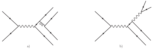
Figure 1: Two representative lowest-order diagrams that contribute to $\Upsilon\to\gamma^{*}\to J/\psi+\chi_{cJ}$. There are totally four diagrams in class a) and two in class b).

We start by considering the decay channel $\Upsilon\to\gamma^{*}\to J/\psi+\chi_{cJ}$, with some typical LO diagrams shown in Fig. 1. This process is very similar to the continuum $J/\psi+\chi_{cJ}$ production in $e^{+}e^{-}$ annihilation Braaten:2002fi .

After obtaining the decay amplitude ${\cal A}^{J}_{\gamma}$ in NRQCD factorization, one can employ the helicity projectors enumerated in Appendix A to project out 10 corresponding helicity amplitudes. It is straightforward to follow equation (10) to read off the reduced helicity amplitude in the single-photon channel:

$$a^{J}_{\gamma;\lambda,\tilde{\lambda}}={N_{c}^{2}-1\over N^{2}_{c}}e_{b}e_{c}\alpha\alpha_{s}\,c^{J}_{\lambda,\tilde{\lambda}}(r),$$ (12)

where $e_{b}=-{1\over 3}$ and $e_{c}={2\over 3}$ are the electric charges of the $b$ and $c$ quarks, $\alpha$ and $\alpha_{s}$ are the QED and QCD coupling constants, respectively. The coefficient functions $c^{J}_{\lambda,\tilde{\lambda}}(r)$ read

$$c^{0}_{0,0}(r)=1+10r-12r^{2}+2ry\qquad c^{0}_{1,0}(r)=9-14r-{y\over 2}\left({1\over r}-6\right),$$ (13a)

$$c^{1}_{0,1}(r)=-\sqrt{6}\left[2-7r+{3\over 2}y\right]\qquad c^{1}_{1,0}(r)=-\sqrt{6}\left[r+{y\over 2}\left({1\over r}-1\right)\right]$$

$$c^{1}_{1,1}(r)=-2\sqrt{6}\left[1-3r+{y\over 4}\left({1\over r}+2\right)\right],$$ (13b)

$$c^{2}_{0,0}(r)=\sqrt{2}[1-2r-12r^{2}+2ry]\qquad c^{2}_{0,1}(r)=\sqrt{6}\left[1-5r+{y\over 2}\right]$$

$$c^{2}_{1,0}(r)=\sqrt{2}\left[3-11r-{y\over 2}\left({1\over r}-3\right)\right]\qquad c^{2}_{1,1}(r)=2\sqrt{6}\left[1-3r-{y\over 4}\left({1\over r}-2\right)\right]$$

$$c^{2}_{1,2}(r)=\sqrt{3}\left[2-{y\over r}\right].$$ (13c)

where $y\equiv-\alpha/\alpha_{s}$. The $y$-dependent terms characterize the photon fragmentation contributions as depicted in Fig. 1b), which are often accompanied by an enhancement factor $1/r$ for the transversely-polarized $J/\psi$.

Barring the pure QED fragmentation contributions, these 10 coefficient functions agree, up to an immaterial phase, with those associated with the process $e^{+}e^{-}\to J/\psi+\chi_{c0,1,2}$ Dong:2011fb  . It is interesting to mention that, for some accidental reason, the QCD part of the single-photon $J/\psi(\pm 1)+\chi_{c1}(0)$ amplitude receives an extra suppression factor than implied from HSR.

III.2 Three-gluon channel

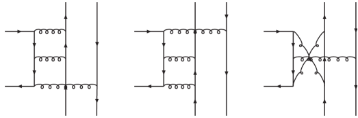
Figure 2: Some representative lowest-order diagrams that contribute to $\Upsilon\to 3g\to J/\psi+\chi_{cJ}$.

Next we turn to the strong decay channel $\Upsilon\to 3g\to J/\psi+\chi_{cJ}$, which supposedly makes the most significant contribution. Some of the representative LO diagrams have been illustrated in Fig. 2. In contrast with the single-photon channel, this channel first starts at the one-loop level. The charge conjugation invariance guarantees that one needs only retain those diagrams with “Abelian” gluon topology as shown in Fig. 2.

After obtaining the decay amplitude ${\cal A}^{J}_{3g}$ using the covariant projection technique, and prior to performing the loop integration, we apply those helicity projection operators given in Appendix A to project out 10 corresponding helicity amplitudes. This operation brings forth great simplification, because all the polarization vectors (tensors) of $\Upsilon$, $J/\psi$ and $\chi_{cJ}$ have been eliminated from the integrand, and the numerators in loop integrals now become Lorentz scalars comprised entirely of the external and loop momenta.

It is then straightforward to utilize the partial fractioning technique to reduce all the higher-point one-loop integrals into a set of 2-point and 3-point scalar integrals. Most of the encountered scalar integrals can be found in the appendix of Ref. Jia:2007hy , whose correctness has been numerically checked by the Mathematica package LoopTools Hahn:1998yk . There also arise some nonstandard 2- and 3-point scalar integrals, which contain propagators with quadratic power due to the projection of the $P$-wave state. All of their analytic expressions can be readily worked out.

As a crosscheck, we also employ the Mathematica package FIRE Smirnov:2008iw and the code Apart Feng:2012iq to perform an independent calculation. Thanks to the integration-by-part (IBP) algorithm built in FIRE, it turns out that all the required master integrals (MIs) become just the conventional 2-point and 3-point scalar integrals as given in Jia:2007hy . The final results generated by this more automatic approach exactly coincides with those obtained from the partial-fractioning method.

As a third consistency check, the calculation is redone by exchanging the order between helicity projection and loop integration. That is, we first utilize the programs Apart and FIRE at the amplitude level, which are more cumbersome and time-consuming, yet still technically feasible. Once the IR-finite $T$-matrices are obtained, we then project out each intended helicity amplitudes at the very end. We again find the exact agreement with the previous two methods. This calculation can be viewed as a strong support for the validity of the 4-dimensional helicity projectors given in Appendix A.

Each individual diagram in Fig. 2, being ultraviolet convergent, albeit contains logarithmic infrared divergence. Dimensional regularization (DR) is adopted to regularize those IR singularities. Upon summing all the diagrams, the ultimate expression for each helicity amplitude becomes IR finite, which endorses the validity of NRQCD factorization approach for these exclusive $\Upsilon$ decay processes.

Following (10), we express the reduced helicity amplitude in the three-gluon channel as

$$a^{J}_{3g;\lambda,\tilde{\lambda}}={(N_{c}^{2}-1)(N_{c}^{2}-4)\over N^{4}_{c}}{\alpha_{s}^{3}\over 8\pi}{m_{b}^{2}\over m_{b}^{2}-4m_{c}^{2}}f^{J}_{\lambda,\tilde{\lambda}}(r).$$ (14)

The color factor reflects the fact the three “Abelian” gluons in Fig. 2 must bear an odd $C$-parity, thus proportional to $d^{abc}d^{abc}=(N_{c}^{2}-1)(N_{c}^{2}-4)/N_{c}$, where $d^{abc}$ denotes the totally symmetric structure constants of $SU(N_{c})$ group.

All the loop effects are encapsulated in the complex-valued dimensionless functions $f^{J}_{\lambda,\tilde{\lambda}}(r)$. Their full expressions are somewhat lengthy, so will not be reproduced here . On the other hand, the profiles of these functions over a wide range of $r$ are explicitly shown in Figs. 3, 4, 5.

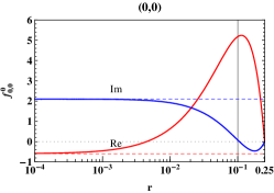
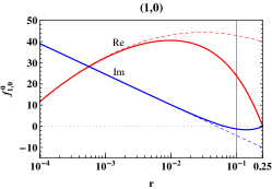
Figure 3: Real and imaginary parts of $f^{0}_{\lambda,\tilde{\lambda}}(r)$. The solid curves correspond to the exact results, and the dashed curves represent the asymptotic ones taken from (15a) and (15b). The vertical mark is placed at the phenomenologically relevant point $r=0.10$.

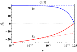
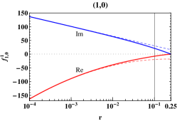
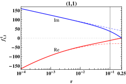
Figure 4: Real and imaginary parts of $f^{1}_{\lambda,\tilde{\lambda}}(r)$. The solid curves correspond to the exact results, and the dashed curves represent the asymptotic ones taken from (15c) to (15e).

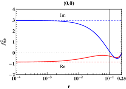
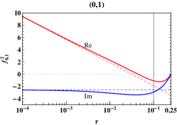
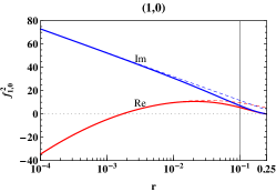
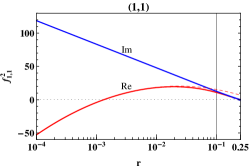
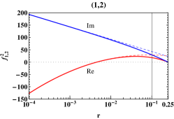
Figure 5: Real and imaginary parts of $f^{2}_{\lambda,\tilde{\lambda}}(r)$. The solid curves correspond to the exact results, and the dashed curves represent the asymptotic ones taken from (15f) to (15j).

Theoretically, it is interesting to ascertain the asymptotic behaviors of these reduced helicity amplitudes in the limit $m_{b}\gg m_{c}$. As mentioned before, we anticipate to see the logarithm scaling violation to the naive power-law scaling given in (8). The asymptotic expressions of the $f^{J}_{\lambda,\tilde{\lambda}}$ functions read ($J=0,1,2$):

$$f^{0}_{0,0}(r) = -4+{2\pi\over 3\sqrt{3}}+{2\pi^{2}\over 9}+{2\pi i\over 3}+{\cal O}(r\ln^{2}{r}),$$ (15a)

$$f^{0}_{1,0}(r) = -\ln^{2}r-7\ln{r}-{\pi^{2}\over 9}+{25\pi\over\sqrt{3}}-{73\over 6}-2\pi i(\ln{r}+3)+{\cal O}(r\ln^{2}{r}),$$ (15b)

$$f^{1}_{0,1}(r) = \sqrt{6}\left({2\over 3}\ln r+{\pi^{2}\over 3}-{17\pi\over 2\sqrt{3}}+{73\over 9}+3\pi i\right)+{\cal O}(r\ln{r}),$$ (15c)

$$f^{1}_{1,0}(r) = \sqrt{6}\left[-\ln^{2}r-3\ln r+{\pi^{2}\over 9}-{8\pi\over\sqrt{3}}+{23\over 6}-2\pi i\left(\ln{r}+{1\over 3}\right)\right]+{\cal O}(r\ln^{2}{r}),$$ (15d)

$$f^{1}_{1,1}(r) = \sqrt{6}\left[-\ln^{2}r-{7\over 2}\ln r-{8\pi^{2}\over 9}-{7\pi\over 3\sqrt{3}}-{25\over 12}-2\pi i\left(\ln{r}-{7\over 6}\right)\right]+{\cal O}(r\ln^{2}{r}),$$ (15e)

$$f^{2}_{0,0}(r) = \sqrt{2}\left({2\pi^{2}\over 9}+{2\pi\over 3\sqrt{3}}-4+{2\pi i\over 3}\right)+{\cal O}(r\ln^{2}{r}),$$ (15f)

$$f^{2}_{0,1}(r) = \sqrt{6}\left(-{2\over 3}\ln r+{5\pi^{2}\over 9}-{7\pi\over 2\sqrt{3}}-{13\over 9}-{\pi i\over 3}\right)+{\cal O}(r\ln^{2}{r}),$$ (15g)

$$f^{2}_{1,0}(r) = \sqrt{2}\left[-\ln^{2}r-7\ln r+{11\pi^{2}\over 9}-{11\pi\over\sqrt{3}}+{23\over 6}-2\pi i(\ln{r}+1)\right]+{\cal O}(r\ln^{2}{r}),$$ (15h)

$$f^{2}_{1,1}(r) = \sqrt{6}\left[-\ln^{2}r-{15\over 2}\ln r-{8\pi^{2}\over 9}+{25\pi\over 3\sqrt{3}}-{145\over 12}-2\pi i\left(\ln{r}+{3\over 2}\right)\right]+{\cal O}(r\ln^{2}{r}),$$

$$f^{2}_{1,2}(r) = \sqrt{3}\left[-2\ln^{2}r-10\ln r+{10\pi^{2}\over 9}-{20\pi\over\sqrt{3}}+{89\over 3}-4\pi i\left(\ln{r}+{1\over 3}\right)\right]+{\cal O}(r\ln^{2}{r}).$$

For readers’ convenience, all the asymptotic results of $f^{J}_{\lambda,\tilde{\lambda}}(r)$ are also shown in Figs. 3, 4, 5, in juxtapose with the corresponding exact results. We observe that for most helicity configurations, the asymptotic results do not coincide well with the exact ones at the phenomenologically relevant point $r=m_{c}^{2}/m_{b}^{2}\approx 0.10$.

From (15), one confirms that the scaling violation is indeed of the logarithmic form. More interestingly, we see that the occurrence of the double-logarithm $\ln^{2}r$ is always affiliated with the helicity-suppressed ($|\lambda+\tilde{\lambda}|>0$) decay channels. This is compatible with the empirical pattern observed in Ref. Jia:2010fw ; Dong:2011fb . Indeed, such double logarithms have previously also been observed in the helicity-suppressed bottomonium exclusive decay processes, e.g. $\Upsilon\to J/\psi+\eta_{c}$ Jia:2007hy , $\eta_{b}\to J/\psi J/\psi$ Gong:2008ue . The light-cone approach is presumably the proper tool to handle these process-dependent double logarithms. Unfortunately, due to some longstanding problems, it remains as a challenge to have a systematic control over these double logarithms appearing in the NRQCD short-distance coefficients Jia:2010fw .

Finally we mention one peculiarity associated with the helicity channel $\Upsilon\rightarrow J/\psi(\lambda=\pm 1)+\chi_{c1}(\tilde{\lambda}=0)$. Recall that at LO in $\alpha_{s}$, this helicity amplitude from the single-photon channel is suppressed by an extra factor of $r$ with respect to the HSR, as can be seen in (13b). Nevertheless, from (15d), we find that this helicity amplitude in the $3g$ channel just possesses the correct power-law scaling as dictated by the HSR. This implies that the power suppression of the LO single-photon amplitude is purely accidental.

III.3 One-photon-two-gluon channel

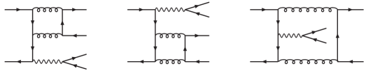
Figure 6: Some representative lowest-order diagrams that contribute to $\Upsilon\to\gamma gg\to J/\psi+\chi_{cJ}$.

From the ratios of the measured inclusive $\Upsilon$ decay rates in three different channels, as listed in (2), an educated guess is that the exclusive decay channel $\Upsilon\to\gamma gg\to J/\psi+\chi_{cJ}$ yields the least important contribution. Nevertheless, for the sake of completeness, let us finally assess the contribution from this radiative decay channel.

Similar to the strong decay channel, this radiative decay channel also starts at the one-loop order. Some typical LO diagrams have been illustrated in Fig. 6. For simplicity, and to be commensurate with the approximation adopted for the single-photon channel in Sec. III.1, we only retain those photon-fragmentation diagrams, whereas the neglected diagrams are the identical as Fig. 2 except with the gluon outside the loop replaced by the photon. We wish that these fragmentation-type diagrams constitute the dominant contributions, which is certainly the case for the transversely-polarized $J/\psi$.

Following the steps outlined in Sec. III.2, one then projects out the 10 required helicity amplitudes, with all the polarization vectors (tensors) of $\Upsilon$, $J/\psi$ and $\chi_{cJ}$ eliminated from the loop integral. Nevertheless, it appears to be much more difficult than in the three-gluon channel to employ the partial fraction to simplify the encountered one-loop integrals.

Fortunately, the powerful Mathematica packages FIRE Smirnov:2008iw and Apart Feng:2012iq can still be successfully applied to reduce the general higher-point tensor one-loop integrals into a set of MIs. With the aid of the IBP algorithm built in FIRE, all the involved MIs become just the standard 2-point and 3-point scalar integrals. The analytic expressions of these scalar integrals can be found in Jia:2007hy ; Ellis:2007qk , whose correctness have been numerically verified by using LoopTools Hahn:1998yk .

Analogous to the three-gluon decay channel, each individual diagram in Fig. 6 is UV finite but IR divergent. After summing all the diagrams, the ultimate expression for each helicity amplitude turns out to be completely IR finite.

In accordance with (10), the reduced helicity amplitude in the radiative decay channel can be expressed as

$$a^{J}_{\gamma gg;\lambda,\tilde{\lambda}}={N_{c}^{2}-1\over N^{2}_{c}}\,{e_{b}e_{c}\alpha\alpha_{s}^{2}\over 4\pi}\,{m_{b}^{2}\over m_{b}^{2}-4m_{c}^{2}}\,r^{-|\lambda|}g^{J}_{\lambda,\tilde{\lambda}}(r),$$ (16)

The inclusion of an extra factor $r^{-|\lambda|}$ is reminiscent of the photon fragmentation mechanism: when the $J/\psi$ becomes transversely polarized ($\lambda=\pm 1$), the corresponding helicity amplitude would receive a $1/r$ enhancement with respect to the nominal HSR.

All the loop effects are encoded in the complex-valued, dimensionless functions $g^{J}_{\lambda,\tilde{\lambda}}(r)$. Their full expressions are somewhat lengthy, and will not be reproduced here. On the other hand, the profiles of these functions over a wide range of $r$ are shown in Figs. 7, 8 and 9.

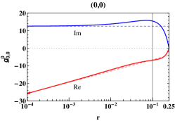
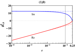
Figure 7: Real and imaginary parts of $g^{0}_{\lambda,\tilde{\lambda}}(r)$. The solid curves correspond to the exact results, and the dashed curves represent the asymptotic ones taken from (17a) and (17b). The vertical mark is placed at the phenomenologically relevant point $r=0.10$.

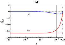
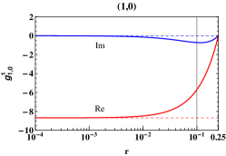
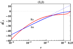
Figure 8: Real and imaginary parts of $g^{1}_{\lambda,\tilde{\lambda}}(r)$. The solid curves correspond to the exact results, and the dashed curves represent the asymptotic ones taken from (17c) to (17e).

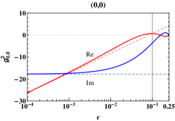
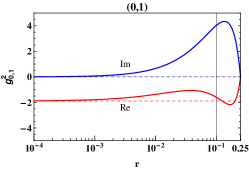
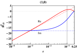
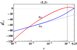
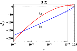
Figure 9: Real and imaginary parts of $g^{2}_{\lambda,\tilde{\lambda}}(r)$. The solid curves correspond to the exact results, and the dashed curves represent the asymptotic ones taken from (17f) to (17j).

It is curious to know the asymptotic behavior of the reduced helicity amplitudes in this decay channel. After some manipulations, we find the asymptotic expressions of the functions $g^{J}_{\lambda,\tilde{\lambda}}$ ($J=0,1,2$) to read

$$g^{0}_{0,0}(r)=4\ln 2\ln r-{\pi^{2}\over 3}-4\ln 2+{53\over 9}+4\pi i+{\cal O}(r\ln^{2}{r}),$$ (17a)

$$g^{0}_{1,0}(r)=4\ln 2\ln r+{5\pi^{2}\over 12}-8\ln 2+1+4\pi i+{\cal O}(r\ln^{2}{r}),$$ (17b)

$$g^{1}_{0,1}(r)=-4\sqrt{6}\left(\ln 2+1\right)+{\cal O}(r\ln{r}),$$ (17c)

$$g^{1}_{1,0}(r)=\sqrt{6}\left(2\ln 2-{\pi^{2}\over 2}\right)+{\cal O}(r\ln{r}),$$ (17d)

$$g^{1}_{1,1}(r)=-\sqrt{6}\left[\frac{1}{2}\ln^{2}r+4\ln 2\ln r+{\pi^{2}\over 12}+8\ln 2-\pi i\left(\ln r+3\right)\right]+{\cal O}(r\ln^{2}{r}),$$ (17e)

$$g^{2}_{0,0}(r)=\sqrt{2}\left(4\ln{2}\ln{r}-{\pi^{2}\over 3}+12\ln 2-{17\over 9}-4\pi i\right)+{\mathcal{O}}(r\ln^{2}r),$$ (17f)

$$g^{2}_{0,1}(r)=\sqrt{6}\left(2-4\ln{2}\right)+{\cal O}(r\ln{r}),$$ (17g)

$$g^{2}_{1,0}(r)=\sqrt{2}\left(4\ln 2\ln r+{5\pi^{2}\over 12}+8\ln 2-3-4\pi i\right)+{\cal O}(r\ln{r}),$$ (17h)

$$g^{2}_{1,1}(r)=\sqrt{6}\left[-\frac{1}{2}\ln^{2}r-4\ln 2\ln r+4\ln r+{5\pi^{2}\over 12}-{20\over 3}\ln 2+{23\over 3}+\pi i\left(\ln r-\frac{5}{3}\right)\right]$$

$$\qquad\quad+{\cal O}(r\ln^{2}{r}),$$ (17i)

$$g^{2}_{1,2}(r)=\sqrt{3}\left[-2\ln^{2}r-4\ln r+{5\pi^{2}\over 6}+{16\over 3}\ln 2-{16\over 3}+2\pi i\left(2\ln{r}+{5\over 3}\right)\right]$$

$$\qquad\quad+{\cal O}(r\ln{r}).$$ (17j)

In Figs. 7, 8, 9, we also juxtapose these asymptotic results of $g^{J}_{\lambda,\tilde{\lambda}}(r)$ with the exact results. For most helicity configurations, the asymptotic results seem not to converge well with the exact ones for the phenomenologically relevant point $r=m_{c}^{2}/m_{b}^{2}\approx 0.10$.

A quick survey on (17) reveals that that the scaling violation is again of the logarithmic form. More interestingly, the same pattern of double logarithms still holds: the occurrence of the double-logarithm $\ln^{2}r$ is always affiliated with the helicity-suppressed decay channels.

We close this section by making a simple observation. As can be seen from Fig. 8, the imaginary parts of the functions $g^{1}_{\lambda,\tilde{\lambda}}$ are generally nonzero, though some of which vanish asymptotically. At first sight, this may contradict Landau-Yang theorem because $\chi_{c1}\to gg$ should be strictly forbidden. This implies that, though the apparent two-gluon cuts in Fig. 6 do not contribute, the other cuts that simultaneously pass through the bottom and charm quark lines must yield nonvanishing contributions to the imaginary parts for $\Upsilon\rightarrow J/\psi+\chi_{c1}$.

IV phenomenology

We are now in a position to make concrete predictions for the decay rates of $\Upsilon\to J/\psi+\chi_{c0,1,2}$, by plugging (12), (14) and (16) into (11).

In the numerical analysis, we take the various bottomonia and charmonia masses from the 2012 PDG compilation Beringer:1900zz : $M_{\Upsilon(1S)}=9.460$ GeV, $M_{\Upsilon(2S)}=10.023$ GeV, $M_{\Upsilon(3S)}=10.355$ GeV, $M_{J/\psi}=3.097$ GeV, $M_{\chi_{c0}}=3.415$ GeV, $M_{\chi_{c1}}=3.511$ GeV, $M_{\chi_{c2}}=3.556$ GeV. These inputs are used to determine $|{\bf P}|$ according to (4), which appears in the phase space factor in (11). To calculate the squared matrix elements, particularly the functions $f^{J}_{\lambda,\widetilde{\lambda}}(r)$ and $g^{J}_{\lambda,\widetilde{\lambda}}(r)$, we instead adopt the following values for the quark masses: $m_{c}=1.5\ \mathrm{GeV}$, $m_{b}=4.7\ \mathrm{GeV}$, corresponding to $r=0.102$. Later we also wish to predict the branching fractions for the decays $\Upsilon(nS)\to J/\psi+\chi_{c0,1,2}$ ($n=1,2,3$). For this purpose, we take the total decay width of various $\Upsilon$ states from Beringer:1900zz : $\Gamma[\Upsilon(1S)]=54.02$ keV, $\Gamma[\Upsilon(2S)]=31.98$ keV, and $\Gamma[\Upsilon(3S)]=20.32$ keV, respectively.

For simplicity, we fix the electromagnetic fine structure constant as $\alpha=1/137$. For the strong coupling constant, any value evaluated with the renormalization scale ranging from $2m_{b}$ to $2m_{c}$ seems to be acceptable. This scale ambiguity constitutes one of the most important sources of theoretical uncertainty. Without much prejudice, we simply choose a medium value $\alpha_{s}(m_{b})=0.22$.

As for the wave functions at the origin for various quarkonia, we use the values obtained from the Buchmüller-Tye potential model Eichten:1995 : $|R_{\Upsilon(1S)}(0)|^{2}=6.477\ \mathrm{GeV}^{3}$, $|R_{\Upsilon(2S)}(0)|^{2}=3.234\ \mathrm{GeV}^{3}$, $|R_{\Upsilon(3S)}(0)|^{2}=2.474\ \mathrm{GeV}^{3}$, $|R_{J/\Psi}(0)|^{2}=0.81\ \mathrm{GeV}^{3}$, $|R^{\prime}_{\chi_{c0,1,2}}(0)|^{2}=0.075\ \mathrm{GeV}^{5}$.

Table 1: The values of the reduced helicity amplitudes $a_{\gamma}$, $a_{3g}$ and $a_{\gamma gg}$ associated with each helicity channel for $\Upsilon(1S)\to J/\psi+\chi_{c0,1,2}$. For simplicity, a factor of $10^{-4}$ has been pulled out of each entry.

		(0,0)	(1,0)	(0,1)	(1,1)	(1,2)
$J/\psi+\chi_{c0}$	$a_{\gamma}$	$-5.99$	$-24.23$	–	–	–
	$a_{3g}$	$18.33e^{i0.54^{\circ}}$	$82.87e^{-i3.19^{\circ}}$	–	–	–
	$a_{\gamma gg}$	$1.58e^{-i66.32^{\circ}}$	$1.01e^{-i58.59^{\circ}}$	–	–	–
$J/\psi+\chi_{c1}$	$a_{\gamma}$	–	$-0.35$	$9.61$	$9.27$	–
	$a_{3g}$	–	$78.04e^{i109.57^{\circ}}$	$54.94e^{i112.26^{\circ}}$	$135.67e^{i108.61^{\circ}}$	–
	$a_{\gamma gg}$	–	$5.23e^{i7.29^{\circ}}$	$1.30e^{i7.48^{\circ}}$	$6.20e^{i20.52^{\circ}}$	–
$J/\psi+\chi_{c2}$	$a_{\gamma}$	$-2.98$	$-8.94$	$-3.68$	$-11.80$	$-12.78$
	$a_{3g}$	$1.15e^{i157.72^{\circ}}$	$30.89e^{i51.71^{\circ}}$	$10.94e^{-i110.67^{\circ}}$	$57.18e^{i49.00^{\circ}}$	$120.16e^{i58.27^{\circ}}$
	$a_{\gamma gg}$	$0.33e^{i101.36^{\circ}}$	$6.89e^{i102.07^{\circ}}$	$0.41e^{-i68.19^{\circ}}$	$14.35e^{i101.39^{\circ}}$	$24.70e^{i103.90^{\circ}}$

In Table 1, we tabulate the values of the reduced helicity amplitudes $a_{\gamma}$, $a_{3g}$ and $a_{\gamma gg}$ associated with each helicity channel for $\Upsilon(1S)\to J/\psi+\chi_{c0,1,2}$. One sees that the relative phases among each amplitude vary channel by channel, and particularly there seems no universal phase pattern between the single-photon and three-gluon channel. Our finding contradicts the universal relative phase conjecture made in Gerard:1999uf .

One curious question is whether the relative strength between three distinct decay mechanisms bears the roughly same pattern as that in $\Upsilon$ inclusive decay, as given in (2). A very crude guess is that each helicity amplitude for this exclusive decay process might be proportional to $\sqrt{{\cal B}_{\rm incl}}$, so that one naively expects

$$|a_{\gamma}|:|a_{3g}|:|a_{\gamma gg}|\approx 1:3.3:0.5,$$ (18)

for each helicity configuration.

Inspecting Table 1, we find that for many helicity configurations, the three distinct helicity amplitudes do exhibit the similar hierarchy as given in (18), i.e., $|a_{3g}|>|a_{\gamma}|>|a_{\gamma gg}|$, though the radiative decay amplitude are often much more suppressed. However, there are also a few notable exceptions, e.g., for the polarized decays $\Upsilon\to J/\psi(\pm 1)+\chi_{c1}(0)$ , $\Upsilon\to J/\psi(\pm 1)+\chi_{c2}(\pm 1)$, $\Upsilon\to J/\psi(\pm 1)+\chi_{c2}(\pm 2)$, the magnitude of the radiative decay amplitudes is comparable, or even greater, than that of the single-photon amplitudes; for the decay $\Upsilon\to J/\psi(0)+\chi_{c2}(0)$, the single-photon amplitude is even greater in magnitude than the respective three-gluon amplitude.

Table 2: The polarized and the polarization-summed partial widths and the corresponding branching fractions. $\Gamma^{[J]}_{\gamma}$, $\Gamma^{[J]}_{3g}$ and $\Gamma^{[J]}_{\gamma gg}$ represent the individual decay rates from the single-photon, three-gluon, and one-photon-two-gluon channels affiliated with the process $\Upsilon(1S)\to J/\psi+\chi_{cJ}$ ($J=0,1,2$), respectively, while $\Gamma^{[J]}_{\rm tot}$ denotes the decay rate which incorporates all three decay mechanisms according to (11). The two rightmost columns also give the unpolarized decay rates and branching fractions by summing over all possible helicity configurations. All the partial decay widths are in units of eV.

	(0,0)	(1,0)	(0,1)	(1,1)	(1,2)	Unpol	${\cal B}$
$\Gamma^{[0]}_{\gamma}$	$4.2\times 10^{-3}$	$7.0\times 10^{-3}$	–	–	–	$1.8\times 10^{-2}$	$3.3\times 10^{-7}$
$\Gamma^{[0]}_{3g}$	$3.9\times 10^{-2}$	$8.2\times 10^{-2}$	–	–	–	$2.0\times 10^{-1}$	$3.7\times 10^{-6}$
$\Gamma^{[0]}_{\gamma gg}$	$2.9\times 10^{-4}$	$1.2\times 10^{-3}$	–	–	–	$2.6\times 10^{-3}$	$4.8\times 10^{-8}$
$\Gamma^{[0]}_{\rm tot}$	$1.4\times 10^{-2}$	$2.8\times 10^{-2}$	–	–	–	$7.0\times 10^{-2}$	$1.3\times 10^{-6}$
$\Gamma^{[1]}_{\gamma}$	–	$1.4\times 10^{-6}$	$1.1\times 10^{-3}$	$1.0\times 10^{-4}$	–	$2.4\times 10^{-3}$	$4.4\times 10^{-8}$
$\Gamma^{[1]}_{3g}$	–	$7.1\times 10^{-2}$	$3.5\times 10^{-2}$	$2.2\times 10^{-2}$	–	$2.6\times 10^{-1}$	$4.8\times 10^{-6}$
$\Gamma^{[1]}_{\gamma gg}$	–	$3.2\times 10^{-4}$	$2.0\times 10^{-5}$	$4.6\times 10^{-5}$	–	$7.7\times 10^{-4}$	$1.4\times 10^{-8}$
$\Gamma^{[1]}_{\rm tot}$	$-$	$6.2\times 10^{-2}$	$4.7\times 10^{-2}$	$2.3\times 10^{-2}$	–	$2.6\times 10^{-1}$	$4.9\times 10^{-6}$
$\Gamma^{[2]}_{\gamma}$	$1.0\times 10^{-3}$	$9.3\times 10^{-4}$	$1.6\times 10^{-4}$	$1.7\times 10^{-4}$	$2.0\times 10^{-5}$	$3.6\times 10^{-3}$	$6.7\times 10^{-8}$
$\Gamma^{[2]}_{3g}$	$1.5\times 10^{-4}$	$1.1\times 10^{-2}$	$1.4\times 10^{-3}$	$3.9\times 10^{-3}$	$1.7\times 10^{-3}$	$3.6\times 10^{-2}$	$6.7\times 10^{-7}$
$\Gamma^{[2]}_{\gamma gg}$	$1.2\times 10^{-5}$	$5.5\times 10^{-4}$	$2.0\times 10^{-6}$	$2.4\times 10^{-4}$	$7.4\times 10^{-5}$	$1.8\times 10^{-3}$	$3.3\times 10^{-8}$
$\Gamma^{[2]}_{\rm tot}$	$5.3\times 10^{-4}$	$2.6\times 10^{-3}$	$5.5\times 10^{-4}$	$1.1\times 10^{-3}$	$8.3\times 10^{-4}$	$1.1\times 10^{-2}$	$2.0\times 10^{-7}$

In Table 2, we also list the polarized decay widths for $\Upsilon(1S)\to J/\psi(\lambda)+\chi_{c0,1,2}(\tilde{\lambda})$ for each independent helicity configurations $(\lambda,\tilde{\lambda})$, together with the polarization-summed results. To readily visualize the interference effect among three distinct decay mechanisms, we also tabulate the individual decay rates from the single-photon, three-gluon, and one-photon-two-gluon channels, respectively, as well as the full decay rate given by (11). Table 2 reveals that $a_{\gamma}$ and $a_{3g}$ in $\Upsilon(1S)\to J/\psi+\chi_{c0,2}$ are subject to destructive interference.

The hierarchy among the polarized decay widths in different helicity configurations, from either an individual decay mechanism or the complete contributions, seems hardly to obey the HSR as indicated in (8). The pattern is abnormal for $\Upsilon\to J/\psi+\chi_{c0}$, where the helicity-suppressed $(\pm 1,0)$ channel even possesses a bigger decay rate than the helicity-favored $(0,0)$ channel; for $\Upsilon\to J/\psi+\chi_{c2}$, the largest polarized decay rates are associated with the helicity-suppressed configurations $(\pm 1,0)$ and $(\pm 1,\pm 1)$, whereas the smallest polarized decay rate is associated with the HSR-favored $(0,0)$ state . These symptoms can presumably be attributed to the fact that the mass ratio $m_{c}/m_{b}\approx 1/3$ might not be small enough to warrant the asymptotic counting rule.

Table 3: The unpolarized partial decay widths and the corresponding branching fractions that incorporate all three distinct decay mechanisms. The superscript $[J]$ characterizes the corresponding decay process $\Upsilon(1S,2S,3S)\to J/\psi+\chi_{cJ}$ ($J=0,1,2$).

	$\Gamma^{[0]}$ (eV)	${\mathcal{B}}^{[0]}$	$\Gamma^{[1]}$ (eV)	${\mathcal{B}}^{[1]}$	$\Gamma^{[2]}$(eV)	${\mathcal{B}}^{[2]}$
$\Upsilon$(1S)	$0.070$	$1.3\times 10^{-6}$	$0.26$	$4.9\times 10^{-6}$	$0.011$	$2.0\times 10^{-7}$
$\Upsilon$(2S)	$0.035$	$1.1\times 10^{-6}$	$0.13$	$4.1\times 10^{-6}$	$0.0054$	$1.7\times 10^{-7}$
$\Upsilon$(3S)	$0.026$	$8.6\times 10^{-7}$	$0.099$	$3.3\times 10^{-6}$	$0.0041$	$1.3\times 10^{-7}$

Finally in Table 3, we tabulate our predictions of the partial decay widths, which are calculated according to (7), together with the corresponding branching fractions, for the various processes $\Upsilon(nS)\to J/\psi+\chi_{c0,1,2}$ ($n=1,2,3$). All the three decay mechanisms are incorporated. We observe that the decay branching fractions satisfy the ordering  ${\cal B}^{[1]}>{\cal B}^{[0]}\gg{\cal B}^{[2]}$, with the first two reaching the order of $10^{-6}$. We note that all these predicted branching ratios are compatible with the various experimental bounds on $J/\psi$ or $\chi_{cJ}$ inclusive production rates in $\Upsilon(1S,2S)$ decays, as given in (1).

As a simple consequence of the LO NRQCD prediction, there should exist a 77% rule in the hadronic decay of the $\Upsilon$ system, in analogy with the famous 12% rule in the $\psi$ system:

$${{\cal B}[\Upsilon(2S)\to{\rm hadrons}]\over{\cal B}[\Upsilon(1S)\to{\rm hadrons}]}={{\cal B}[\Upsilon(2S)\to e^{+}e^{-}]\over{\cal B}[\Upsilon(1S)\to e^{+}e^{-}]}=0.77\pm 0.07.$$ (19)

Not surprisingly, the ratios of ${\cal B}[\Upsilon(2S)\to J/\psi+\chi_{cJ}]$ to ${\cal B}[\Upsilon(1S)\to J/\psi+\chi_{cJ}]$ in Table 3 are indeed compatible with this rule.

Thus far, the Belle experiment has collected about $102$ million $\Upsilon(1S)$ samples and $158$ million $\Upsilon(2S)$ samples. According to Table 3, the Belle experiment is expected to have produced about 130 and 170 $\Upsilon(1S,2S)\to J/\psi+\chi_{c0}$ events, 500 and 650 $\Upsilon(1S,2S)\to J/\psi+\chi_{c1}$ events, 20 and 30 $\Upsilon(1S,2S)\to J/\psi+\chi_{c2}$ events, respectively.

Experimentally, there are two possible methods to detect the $J/\psi+\chi_{c0,1,2}$ signals. The first is to reconstruct both the $J/\psi$ and $\chi_{c0,1,2}$ events. The clean and copious decay modes of $\chi_{c1,2}$ are the $E1$ radiative transitions $\chi_{c1,2}\to J/\psi+\gamma$, with the branching fractions of $34.4$% and $19.5$%, respectively Beringer:1900zz . The $J/\psi$ meson can be most cleanly tagged through the leptonic decays into $e^{+}e^{-}$ and $\mu^{+}\mu^{-}$, with combined branching ratios about 12% Beringer:1900zz . Although this method has the advantage of bearing very low background level, taking into account the reconstruction efficiencies for two $J/\psi$ and one photon, one may end up with too few signal events to be practically useful.

The second method is to only reconstruct one $J/\psi\to l^{+}l^{-}$ event, then fit the recoil mass spectrum against the $J/\psi$ to estimate the number of $\chi_{c0,1,2}$ peak events. This method will not depend on the concrete decay modes of $\chi_{c0,1,2}$. For low statistics of signal events like in our case, this method is much more superior to the preceding one. As a matter of fact, this method has already been used by the Belle collaboration to impose the upper bound for the exclusive bottomonium decays $\chi_{b0,1,2}\to J/\psi J/\psi,J/\psi\psi^{\prime}$ Shen:2012ei .

In fitting the recoil mass spectrum of $J/\psi$, the net detection efficiency for $\Upsilon(1S,2S)\to J/\psi+\chi_{c0,1,2}$ is estimated to be around 4% (similar for all $\chi_{c0,1,2}$), with the reconstruction efficiency for $J/\psi\to l^{+}l^{-}$ included Shen:2012:private . Therefore, the numbers of the observed $\Upsilon(1S,2S)\to J/\psi+\chi_{c1}$ events are expected to be $500\times 4\%=20$, and $650\times 4\%=26$, respectively. Since only one $J/\psi$ is reconstructed, the background level in real data may not be very low. With only 20 reconstructed signal events, it seems quite challenging for the signal significance to reach the $5\sigma$ level, and a larger data pool is needed in order to draw a definite conclusion. In the prospective Super $B$ factory, with a luminosity 50 times greater than the current $B$ factory, it seems very promising that the decays $\Upsilon(1S,2S,3S)\to J/\psi+\chi_{c0,1}$ will be eventually observed.

V Summary

In this paper, we carry out a comprehensive investigation on the exclusive $J/\psi+\chi_{c0,1,2}$ production in $\Upsilon$ decay in the NRQCD factorization framework. We have explicitly considered three distinct decay mechanisms, i.e., the strong, electromagnetic and radiative decay channels. Although there has not yet appeared a rigorous proof on the validity of NRQCD factorization approach to these types of double-charmonium production processes, the explicit verification for the cancelation of IR divergences in our calculation is rather supportive of the positive answer. Moreover, our explicit calculation further supports the previous claim that the double logarithms appearing in the one-loop NRQCD short-distance coefficients are always affiliated with the helicity-suppressed channels Jia:2010fw ; Dong:2011fb .

The branching fractions for the various polarized and unpolarized decay channels $\Upsilon(nS)\to J/\psi+\chi_{c0,1,2}$ ($n=1,2,3$) are predicted by incorporating all three distinct decay channels at the lowest order. In our case, the relative phase among these decay channels arise from the short-distance loop effect, which can actually be calculated in perturbation theory. There appears no universal interference pattern, but the three-gluon and the single-photon amplitudes often tend to be destructive. We find that $\Upsilon(nS)$ decays into $J/\psi+\chi_{c1}$ have the largest branching fraction, about a few times $10^{-6}$; and the decays $\Upsilon(nS)\to J/\psi+\chi_{c2}$ have the smallest decay branching ratio, only of order $10^{-7}$. The current statistics at Belle is on the margin of observing these decay channels. If the prospective high-luminosity $e^{+}e^{-}$ facilities such as the Super B experiment can dedicate more machine time on the first three $\Upsilon$ resonances, it should be an ideal place to discover their exclusive decay modes into $J/\psi+\chi_{c0,1}$.

Appendix A Various helicity projectors for $\Upsilon\to J/\psi+\chi_{c0,1,2}$

During this work, we have utilized the various helicity projectors to expedite projecting out the corresponding helicity amplitudes associated with $\Upsilon\to J/\psi+\chi_{c0,1,2}$. This helicity projection technique, which has already been applied in our previous work on the ${\mathcal{O}}(\alpha_{s})$ correction to the process $e^{+}e^{-}\to J/\psi+\chi_{c0,1,2}$ Dong:2011fb , can significantly reduce the amount of labors required for the loop diagram calculations. In this Appendix, we collect the explicit formulas for the 10 helicity projectors used in this work.

Firstly, it is convenient to introduce the transverse metric tensor:

$$g_{\perp\>\mu\nu} \equiv g_{\mu\nu}+{P_{\mu}P_{\nu}\over|{\bf P}|^{2}}-{Q\cdot P\over M^{2}_{\Upsilon}|{\bf P}|^{2}}(P_{\mu}Q_{\nu}+Q_{\mu}P_{\nu})+{M_{J/\psi}^{2}\over M^{2}_{\Upsilon}}{Q_{\mu}Q_{\nu}\over|{\bf P}|^{2}}$$ (20)

$$= g_{\mu\nu}+{\widetilde{P}_{\mu}\widetilde{P}_{\nu}\over|{\bf P}|^{2}}-{Q\cdot\widetilde{P}\over M^{2}_{\Upsilon}|{\bf P}|^{2}}(\widetilde{P}_{\mu}Q_{\nu}+Q_{\mu}\widetilde{P}_{\nu})+{M_{\chi_{cJ}}^{2}\over M^{2}_{\Upsilon}}{Q_{\mu}Q_{\nu}\over|{\bf P}|^{2}},$$

where $Q$, $P$ and $\widetilde{P}$ stand for the four-momenta of $\Upsilon$, $J/\psi$ and $\chi_{cJ}$, respectively. This symmetric tensor satisfies the transversity condition $g_{\perp\>\mu\nu}P^{\mu}=g_{\perp\>\mu\nu}\widetilde{P}^{\mu}=0$. It further has the properties $g_{\perp\>\mu}^{\;\;\mu}=2$, $g_{\perp\>\mu\alpha}\,g_{\perp}^{\alpha\nu}=g_{\perp\>\mu\alpha}\,g^{\alpha\nu}=g_{\perp\>\mu}^{\;\;\;\nu}$.

The decay amplitude ${\mathcal{A}}^{0}$ for the process $\Upsilon\rightarrow J/\psi+\chi_{c0}$ can be parameterized as ${\mathcal{A}}^{0}={\mathcal{A}}_{\mu\nu}^{0}\epsilon^{\mu}_{\Upsilon}\epsilon^{*\nu}_{J/\psi}(\lambda)$, where $\epsilon_{\Upsilon}$ and $\epsilon_{J/\psi}$ denote the polarization vectors of $\Upsilon$ and $J/\psi$, respectively. The helicities of $J/\psi$ and $\chi_{c0}$ are labeled by $\lambda$ and $\tilde{\lambda}$ (trivially $\tilde{\lambda}=0$). There are only two independent helicity amplitudes for this process, which can be deduced by acting the corresponding helicity projectors on the amputated amplitude: ${\mathcal{A}}_{\lambda,\tilde{\lambda}}^{0}={\mathbb{P}}_{\lambda,\tilde{\lambda}}^{\mu\nu}\,{\mathcal{A}}_{\mu\nu}^{0}$, up to an immaterial phase. The two helicity projection tensors for $\Upsilon\rightarrow J/\psi+\chi_{c0}$ are

$${\mathbb{P}}_{0,0}^{\mu\nu} = {1\over|{\bf P}|^{2}}\bigg{(}P_{\mu}-{Q\cdot P\over M^{2}_{\Upsilon}}Q_{\mu}\bigg{)}\bigg{(}{Q\cdot P\over M_{J/\psi}M_{\Upsilon}}P_{\nu}-{M_{J/\psi}\over M_{\Upsilon}}Q_{\nu}\bigg{)},$$ (21a)

$${\mathbb{P}}_{1,0}^{\mu\nu} = -{1\over 2}\,g_{\perp\>\mu\nu},$$ (21b)

where $g_{\perp\>\mu\nu}$ is defined in (20). These two projectors are normalized as ${\mathbb{P}}_{0,0;\mu\nu}\,{\mathbb{P}}_{0,0}^{\mu\nu}=1$, ${\mathbb{P}}_{1,0;\mu\nu}\,{\mathbb{P}}_{1,0}^{\mu\nu}=\frac{1}{2}$, and orthogonal to each other: ${\mathbb{P}}_{0,0;\mu\nu}\,{\mathbb{P}}_{1,0}^{\mu\nu}=0$.

The decay amplitude ${\mathcal{A}}^{1}$ for the decay process $\Upsilon\rightarrow J/\psi+\chi_{c1}$ can be expressed as ${\mathcal{A}}^{1}={\mathcal{A}}_{\mu\nu\alpha}^{1}\epsilon^{\mu}_{\Upsilon}\epsilon^{*\nu}_{J/\psi}(\lambda)\epsilon^{*\alpha}_{\chi_{c1}}(\tilde{\lambda})$, where $\tilde{\lambda}$ and $\epsilon_{\chi_{c1}}$ denote the helicity of the $\chi_{c1}$ state and the corresponding polarization vector. There are three independent helicity amplitudes for this process, which can be deduced by acting the corresponding helicity projectors on the amputated amplitude: ${\mathcal{A}}_{\lambda,\tilde{\lambda}}^{1}={\mathbb{P}}_{\lambda,\tilde{\lambda}}^{\mu\nu\alpha}\,{\mathcal{A}}_{\mu\nu\alpha}^{1}$. The three helicity projection tensors for $\Upsilon\rightarrow J/\psi+\chi_{c1}$ read:

$${\mathbb{P}}_{1,0}^{\mu\nu\alpha} = {i\over 2M_{\Upsilon}|{\bf P}|^{2}}\,\epsilon_{\mu\nu\rho\sigma}Q^{\rho}\widetilde{P}^{\sigma}\left({Q\cdot\widetilde{P}\over M_{\chi_{c1}}M_{\Upsilon}}{\tilde{P}}_{\alpha}-{M_{\chi_{c1}}\over M_{\Upsilon}}Q_{\alpha}\right),$$ (22a)

$${\mathbb{P}}_{0,1}^{\mu\nu\alpha} = -{i\over 2M_{\Upsilon}|{\bf P}|^{2}}\,\epsilon_{\mu\alpha\rho\sigma}Q^{\rho}P^{\sigma}\left({Q\cdot P\over M_{J/\psi}M_{\Upsilon}}P_{\nu}-{M_{J/\psi}\over M_{\Upsilon}}Q_{\nu}\right),\$$ (22b)

$${\mathbb{P}}_{1,1}^{\mu\nu\alpha} = {i\over 2M_{\Upsilon}|{\bf P}|^{2}}\,\epsilon_{\nu\alpha\rho\sigma}Q^{\rho}P^{\sigma}\left(P_{\mu}-{Q\cdot P\over M^{2}_{\Upsilon}}Q_{\mu}\right),$$ (22c)

which are subject to the normalization conditions ${\mathbb{P}}_{i;\mu\nu\alpha}\,{\mathbb{P}}_{j}^{\mu\nu\alpha}={1\over 2}\delta_{ij}$, with $i$, $j$ signifying one of the three helicity configurations.

Similarly, for the decay process $\Upsilon\rightarrow J/\psi+\chi_{c2}$, we can identify the amputated amplitude through ${\mathcal{A}}^{2}={\mathcal{A}}_{\mu\nu\alpha\beta}^{2}\epsilon^{\mu}_{\Upsilon}\epsilon^{*\nu}_{J/\psi}(\lambda)e^{*\alpha\beta}_{\chi_{c2}}(\tilde{\lambda})$, where $\tilde{\lambda}$ and $e_{\chi_{c2}}$ represent the helicity of the $\chi_{c2}$ state and the corresponding polarization tensor. There are in total five independent helicity amplitudes, which can be obtained by acting the corresponding helicity projectors upon the amputated amplitude: ${\mathcal{A}}_{\lambda,\tilde{\lambda}}^{2}={\mathbb{P}}_{\lambda,\tilde{\lambda}}^{\mu\nu\alpha\beta}\,{\mathcal{A}}_{\mu\nu\alpha\beta}^{2}$. We construct the five helicity projection tensors for $\Upsilon\rightarrow J/\psi+\chi_{c2}$ as

$${\mathbb{P}}_{0,0}^{\mu\nu\alpha\beta} = {1\over\sqrt{6}|{\bf P}|^{2}}\bigg{(}{Q\cdot P\over M_{J/\psi}M_{\Upsilon}}P_{\nu}-{M_{J/\psi}\over M_{\Upsilon}}Q_{\nu}\bigg{)}\bigg{(}P_{\mu}-{Q\cdot P\over M^{2}_{\Upsilon}}Q_{\mu}\bigg{)}\Bigg{[}g_{\perp\>\alpha\beta}+{2\over|{\bf P}|^{2}}$$ (23a)

$$\times\bigg{(}{Q\cdot\widetilde{P}\over M_{\chi_{c2}}M_{\Upsilon}}{\widetilde{P}}_{\alpha}-{M_{\chi_{c2}}\over M_{\Upsilon}}Q_{\alpha}\bigg{)}\bigg{(}{Q\cdot\widetilde{P}\over M_{\chi_{c2}}M_{\Upsilon}}{\widetilde{P}}_{\beta}-{M_{\chi_{c2}}\over M_{\Upsilon}}Q_{\beta}\bigg{)}\Bigg{]},$$

$${\mathbb{P}}_{1,0}^{\mu\nu\alpha\beta} = -{1\over 2\sqrt{6}}\,g_{\perp\>\mu\nu}\Bigg{[}g_{\perp\>\alpha\beta}+{2\over|{\bf P}|^{2}}\bigg{(}{Q\cdot\tilde{P}\over M_{\chi_{c2}}M_{\Upsilon}}{\widetilde{P}}_{\alpha}-{M_{\chi_{c2}}\over M_{\Upsilon}}Q_{\alpha}\bigg{)}\bigg{(}{Q\cdot\tilde{P}\over M_{\chi_{c2}}M_{\Upsilon}}{\widetilde{P}}_{\beta}-{M_{\chi_{c2}}\over M_{\Upsilon}}Q_{\beta}\bigg{)}\Bigg{]},$$

$${\mathbb{P}}_{0,1}^{\mu\nu\alpha\beta} = {1\over 2\sqrt{2}|{\bf P}|^{2}}\bigg{(}{Q\cdot P\over M_{J/\psi}M_{\Upsilon}}P_{\nu}-{M_{J/\psi}\over M_{\Upsilon}}Q_{\nu}\bigg{)}\Bigg{[}g_{\perp\>\mu\alpha}\bigg{(}{Q\cdot\widetilde{P}\over M_{\chi_{c2}}M_{\Upsilon}}{\widetilde{P}}_{\beta}-{M_{\chi_{c2}}\over M_{\Upsilon}}Q_{\beta}\bigg{)}$$ (23c)

$$+(\alpha\leftrightarrow\beta)\Bigg{]},$$

$${\mathbb{P}}_{1,1}^{\mu\nu\alpha\beta} = -{1\over 2\sqrt{2}|{\bf P}|^{2}}\bigg{(}P_{\mu}-{Q\cdot P\over M^{2}_{\Upsilon}}Q_{\mu}\bigg{)}\Bigg{[}g_{\perp\>\nu\alpha}\bigg{(}{Q\cdot\widetilde{P}\over M_{\chi_{c2}}M_{\Upsilon}}{\widetilde{P}}_{\beta}-{M_{\chi_{c2}}\over M_{\Upsilon}}Q_{\beta}\bigg{)}+(\alpha\leftrightarrow\beta)\Bigg{]},$$ (23d)

$${\mathbb{P}}_{1,2}^{\mu\nu\alpha\beta} = {1\over 4}(g_{\perp\>\mu\nu}\,g_{\perp\>\alpha\beta}-g_{\perp\>\mu\alpha}\,g_{\perp\>\nu\beta}-g_{\perp\>\mu\beta}\,g_{\perp\>\nu\alpha}).$$ (23e)

These five projection operators satisfy the normalization conditions ${\mathbb{P}}_{i;\mu\nu\alpha\beta}\,{\mathbb{P}}_{j;}^{\mu\nu\alpha\beta}=\frac{1}{2}\delta_{ij}$ ($i$, $j$ corresponding to one of the five helicity configurations), except that ${\mathbb{P}}_{0,0;\mu\nu\alpha\beta}\,{\mathbb{P}}_{0,0}^{\mu\nu\alpha\beta}=1$.

All the helicity projectors are derived by obeying the exact decay kinematics. Nevertheless, in this work we only target at the LO accuracy in $v$ expansion. Therefore, Upon applying these projectors to infer the intended helicity amplitudes, it is eligible to make the following substitutions for the various quarkonium masses: $M_{\Upsilon(nS)}\approx 2m_{b}$ ($n=1,2,3$), and $M_{J/\psi}\approx M_{\chi_{c0,1,2}}\approx 2m_{c}$. Implementing these approximations considerably simplifies the corresponding loop calculation.

References

• (1) J. Beringer et al. [Particle Data Group Collaboration], Phys. Rev. D 86, 010001 (2012).
• (2) C. P. Shen et al. [Belle Collaboration], Phys. Rev. D 86, 031102 (2012) [arXiv:1205.1246 [hep-ex]].
• (3) Y. Jia, Phys. Rev.  D 78, 054003 (2008) [arXiv:hep-ph/0611130].
• (4) B. Gong, Y. Jia and J. X. Wang, Phys. Lett.  B 670 (2009) 350 [arXiv:0808.1034 [hep-ph]].
• (5) V. V. Braguta and V. G. Kartvelishvili, Phys. Rev.  D 81 (2010) 014012 [arXiv:0907.2772 [hep-ph]].
• (6) P. Sun, G. Hao and C. F. Qiao, Phys. Lett.  B 702, 49 (2011) [arXiv:1005.5535 [hep-ph]].
• (7) V. V. Braguta, A. K. Likhoded and A. V. Luchinsky, Phys. Rev. D 72, 094018 (2005) [arXiv:hep-ph/0506009].
• (8) V. V. Braguta, A. K. Likhoded and A. V. Luchinsky, Phys. Rev. D 80, 094008 (2009) [Erratum-ibid. D 85, 119901 (2012)] [arXiv:0902.0459 [hep-ph]].
• (9) J. Zhang, H. Dong and F. Feng, Phys. Rev. D 84, 094031 (2011) [arXiv:1108.0890 [hep-ph]].
• (10) W. -L. Sang, R. Rashidin, U-R. Kim and J. Lee, Phys. Rev. D 84, 074026 (2011) [arXiv:1108.4104 [hep-ph]].
• (11) L. -B. Chen and C. -F. Qiao, JHEP 1211, 168 (2012) [arXiv:1204.0215 [hep-ph]].
• (12) B. A. Irwin, B. Margolis and H. D. Trottier, Phys. Rev. D 42, 1577 (1990).
• (13) Y. Jia, Phys. Rev.  D 76 (2007) 074007 [arXiv:0706.3685 [hep-ph]].
• (14) K. Abe et al. [Belle Collaboration], Phys. Rev. Lett.  89, 142001 (2002), [arXiv:hep-ex/0205104].
• (15) K. Abe et al. [Belle Collaboration], Phys. Rev.  D 70, 071102 (2004) [arXiv:hep-ex/0407009].
• (16) B. Aubert et al. [BABAR Collaboration], Phys. Rev.  D 72, 031101 (2005) [arXiv:hep-ex/0506062].
• (17) E. Braaten and J. Lee, Phys. Rev. D 67, 054007 (2003) [arXiv:hep-ph/0211085].
• (18) K. Y. Liu, Z. G. He and K. T. Chao, Phys. Lett.  B 557, 45 (2003) [arXiv:hep-ph/0211181].
• (19) K. Hagiwara, E. Kou and C. F. Qiao, Phys. Lett.  B 570 (2003) 39 [arXiv:hep-ph/0305102].
• (20) J. P. Ma and Z. G. Si, Phys. Rev.  D 70, 074007 (2004) [arXiv:hep-ph/0405111].
• (21) A. E. Bondar and V. L. Chernyak, Phys. Lett.  B 612, 215 (2005) [arXiv:hep-ph/0412335].
• (22) G. T. Bodwin, D. Kang and J. Lee, Phys. Rev.  D 74, 114028 (2006) [arXiv:hep-ph/0603185].
• (23) Y. -J. Zhang, Y. -j. Gao, K. -T. Chao, Phys. Rev. Lett.  96, 092001 (2006). [hep-ph/0506076].
• (24) B. Gong and J. X. Wang, Phys. Rev.  D 77, 054028 (2008) [arXiv:0712.4220 [hep-ph]].
• (25) Z. G. He, Y. Fan and K. T. Chao, Phys. Rev.  D 75, 074011 (2007) [arXiv:hep-ph/0702239].
• (26) G. T. Bodwin, J. Lee and C. Yu, Phys. Rev.  D 77, 094018 (2008) [arXiv:0710.0995 [hep-ph]].
• (27) V. V. Braguta, Phys. Rev. D 79, 074018 (2009) [arXiv:0811.2640 [hep-ph]].
• (28) For a recent review on $e^{+}e^{-}\to J/\psi+\eta_{c}$ at $B$ factory, see N. Brambilla et al., Eur. Phys. J.  C 71, 1534 (2011).
• (29) H. -R. Dong, F. Feng and Y. Jia, Phys. Rev. D 85, 114018 (2012) [arXiv:1204.4128 [hep-ph]].
• (30) Y. -J. Zhang, Y. -Q. Ma and K. -T. Chao, Phys. Rev. D 78, 054006 (2008) [arXiv:0802.3655 [hep-ph]].
• (31) K. Wang, Y. -Q. Ma, K. -T. Chao, Phys. Rev.  D84, 034022 (2011).
• (32) H. R. Dong, F. Feng and Y. Jia, JHEP 1110 (2011) 141.
• (33) G. T. Bodwin, E. Braaten and G. P. Lepage, Phys. Rev.  D 51, 1125 (1995) [Erratum-ibid.  D 55, 5853 (1997)] [arXiv:hep-ph/9407339].
• (34) J. Xu, Ph.D. thesis, Electromagnetic transitions of quarkonia and productions of $P$-wave quarkonia, IHEP (2011) (in Chinese).
• (35) G. Lopez Castro, J. L. Lucio M. and J. Pestieau, AIP Conf. Proc. 342, 441 (1995) [arXiv:hep-ph/9902300].
• (36) R. Baldini et al., Phys. Lett.  B 444, 111 (1998).
• (37) M. Suzuki, Phys. Rev.  D 60, 051501 (1999) [arXiv:hep-ph/9901327].
• (38) P. Wang, C. Z. Yuan and X. H. Mo, Phys. Rev.  D 69, 057502 (2004) [arXiv:hep-ph/0303144].
• (39) C. Z. Yuan, P. Wang and X. H. Mo, Phys. Lett.  B 567, 73 (2003) [arXiv:hep-ph/0305259].
• (40) S. Dobbs et al. [CLEO Collaboration], Phys. Rev.  D 74, 011105 (2006) [arXiv:hep-ex/0603020].
• (41) M. Jacob and G. C. Wick, Annals Phys.  7 (1959) 404 [Annals Phys.  281 (2000) 774]. Haber:1994pe
• (42) H. E. Haber, In *Stanford 1993, Spin structure in high energy processes* 231-272 [hep-ph/9405376].
• (43) S. J. Brodsky and G. P. Lepage, Phys. Rev.  D 24, 2848 (1981).
• (44) G. P. Lepage and S. J. Brodsky, Phys. Rev. D 22, 2157 (1980).
• (45) V. L. Chernyak and A. R. Zhitnitsky, Phys. Rept.  112, 173 (1984);
• (46) G. T. Bodwin, X. Garcia i Tormo and J. Lee, Phys. Rev. Lett.  101, 102002 (2008) [arXiv:0805.3876 [hep-ph]].
• (47) T. Hahn and M. Perez-Victoria, Comput. Phys. Commun.  118, 153 (1999).
• (48) A. V. Smirnov, JHEP 0810, 107 (2008). [arXiv:0807.3243 [hep-ph]].
• (49) F. Feng, Comput. Phys. Commun.  183, 2158 (2012) [arXiv:1204.2314 [hep-ph]].
• (50) Y. Jia, J. X. Wang and D. Yang, JHEP 1110, 105 (2011).
• (51) R. K. Ellis and G. Zanderighi, JHEP 0802, 002 (2008) [arXiv:0712.1851 [hep-ph]]. Also see the website http://qcdloop.fnal.gov.
• (52) E. J. Eichten and C. Quigg, Phys. Rev. D 52, 1726 (1995).
• (53) J. M. Gerard and J. Weyers, Phys. Lett.  B 462, 324 (1999) [arXiv:hep-ph/9906357].
• (54) C. P. Shen et al. [Belle Collaboration], Phys. Rev. D 85, 071102 (2012) [arXiv:1203.0368 [hep-ex]].
• (55) C. P. Shen, private communication.