Understanding and controlling $N$-dimensional quantum walks via dispersion relations. Application to the 2D and 3D Grover walks: Diabolical points and more

Abstract

The discrete quantum walk in $N$ dimensions is analyzed from the perspective of its dispersion relations. This allows understanding known properties, as well as designing new ones when spatially extended initial conditions are considered. This is done by deriving wave equations in the continuum, which are generically of the Schrödinger type, and allow devising interesting behaviors, such as ballistic propagation without deformation, or the generation of almost flat probability distributions, what is corroborated numerically. There are however special points where the energy surfaces display intersections and, near them, the dynamics is entirely different. Applications to the two- and three-dimensional Grover walks are presented.

I Introduction

Quantum walks (QWs) are becoming widespread in physics. Originally introduced as quantum versions of random classical processes Aharonov93 and quantum cellular automata Meyer96 , they have been deeply investigated, specially in connection with quantum information science Watrous01 ; Nayak00 ; Ambainis03 ; Kempe03 ; Kendon06 ; Kendon06b ; Konno08 , and have been recently shown to constitute a universal model for quantum computation prl102 ; pra81 . Remarkably, along the last decade this simple quantum diffusion model has found connections with very diverse phenomena such as optical diffraction and other wave phenomena Knightc ; German , quantum games Flitney12 , Anderson localization and quantum chaos Buerschaper ; Wojcik ; Romanelli ; Romanelli2012 , and has even been identified as a generalized quantum measurement device Kurzynski12 . Moreover, through proposals for and actual implementations, QWs have found connections with the dynamics of quite different physical systems such as linear optical systems and optical cavities Bouwmester ; Knight ; Jeong03 ; Knightb ; Roldan ; Do ; Banuls ; Perets08 ; Schreiber , optical lattices Dur02 ; Eckert05 ; Chandrashekar08 ; Science , trapped ions Travaglione02 ; Schmitz ; Zaehringer , and Bose-Einstein condensates Chandrashekar06 among others. Along these recent years the experimental capabilities in performing QWs have increased steadily and nowadays there are devices that, e.g., implement two dimensional QWs with a large number of propagation steps Schreiber12 . For recent reviews on the field see Buzek11 ; Venegas12 .

Recently, some of us have been insisting in the interest of analyzing the dynamics of coined QWs from the perspective of their dispersion relation German ; Roldan12 , which has been also used for purposes different to ours (see, e.g., Kempf09 ; Stefanak12 ). We think this is an interesting approach that is particularly suitable for non localized initial conditions, i.e., when the initial state is described by a probability distribution extending on a finite region in the lattice. When this region is not too small, the evolution of the QW can be derived, to a good degree of approximation, from familiar linear differential wave equations. Certainly the use of extended initial conditions has been rare up to now Machida , but we think it is worth insisting in that they allow to reach final probability distributions which, interestingly, can be tailored to some extent. It is also worth mentioning that extended initial conditions also make a connection with multiparticle quantum walks for noninteracting particles Rohde11 .

In Roldan12 we have recently applied the above viewpoint in studying alternate QWs DiFranco11 in $N$ dimensions. Alternate QWs are a simpler version of multidimensional QWs than the standard one Mackay as they only require a single qubit as a coin (used $N$ times per time step) DiFranco11 instead of using a 2$N$-qudit as the coin (used once per time step), as originally defined in Mackay . Here we shall carry out, from the dispersion relation viewpoint, the study of multidimensional QWs in their standard form. Below we make a general treatment, valid for $N$ dimensions, and illustrate our results with the special cases of the Grover two- and three-dimensional QWs. We notice that the 2D Grover-QW has received most of the theoretical attention paid to multidimensional QWs Mackay ; Tregenna03 ; Shenvi ; Inui04 ; Carneiro ; Adamczak ; Marquezino ; Venegas2 ; Watabe ; Oliveira ; Omar ; Stefanak10 ; Stefanak08 .

We shall derive continuous wave equations, whose form depend on the probability distribution at time $t=0$. To the leading order, these equations are partial differential equations that can be written in the form

$$\mathrm{i}\frac{\partial A^{\left(s\right)}\left(\mathbf{X},t\right)}{\partial t}=-\frac{1}{2}\sum_{i,j=1}^{N}\varpi_{ij}^{\left(s\right)}\frac{\partial^{2}A^{\left(s\right)}}{\partial X_{i}\partial X_{j}}+\cdots,$$ (1)

with $A^{\left(s\right)}$ a continuous amplitude probability, coefficients $\varpi_{ij}^{\left(s\right)}$ determined by the QW dispersion relation properties, and $X_{i}$ are the spatial coordinates in a reference frame moving with the group velocity (see below for full details). There is a lot of accumulated knowledge regarding the solutions of the above continuous equations and this knowledge allows, to some extent, for a qualitative knowledge of the long term probability distribution of the QW for particular initial conditions. This qualitative knowledge is particularly appealing to us, as we are interested, not in obtaining approximate continuous solutions to the discrete QW, but in getting a quick intuition of the QW evolution for different initial probability distributions. This allows, in particular, to reach a desired asymptotic distribution by suitably tailoring the initial (extended) state German . Of course, this qualitative knowledge will be only approximate (as the continuous solutions are strictly valid only for infinitely extended initial distributions) but, as we show below, even for relatively narrow initial distributions the qualitative knowledge turns out to be quite accurate. In each case, we will present an exact numerical simulation, obtained from the discrete map of the QW, that illustrates the agreement with the qualitative analysis described above. As far as we know, this is the first time that continuous approximations to the discrete QW are derived for a multidimensional QW.

The continuous equations we derive, however, cannot apply near degeneracies in the dispersion relations, as in their vicinity the eigensolutions of the QW vary wildly from point to point. Hence, close to degeneracies a specific treatment is necessary and we develop such a treatment for a particular type of degeneracies, namely conical intersections. We apply this treatment to the two–dimensional Grover walk that exhibits such conical intersections in the dispersion relation, a fact that seems to have been noticed only recently Roldan12 and that we study here in mathematical detail. These conical intersections, called diabolical points Berry1 ; Berry2 ; Berry3 , determine a type of dynamics similar to that of massless Dirac fermions or of electrons in graphene graphene1 ; graphene2 ; Ohta ; Pleti ; CastroNeto and appear in very different systems: quantum triangular billiards Berry1 , conical refraction in crystal optics Berry2 ; Berry3 , the already mentioned graphene electrons graphene1 ; graphene2 ; Ohta ; Pleti ; CastroNeto , the spectra of polyatomic molecules Mead79 ; Cederbaum03 , optical lattices Zhang or acoustic surface waves Torrent12 , just to mention a few. In all cases the remarkable physical properties exhibited by these systems are directly associated with the existence of the diabolical points. In the three–dimensional Grover walk we also find degeneracies, but these are different to the diabolical points. Diabolical points on the dispersion relations play also a role on the analysis of topological properties of the QW. Configurations with different topologies or Chern numbers can be manufactured, for example, by introducing a spatial variation of one of the coin angles in alternate QW’s, such that these regions possess different topologies. At the boundaries delimiting those regions the gap in the dispersion relation closes, and one can observe the formation of bound states or unidirectionally propagating modes, which are protected by topological invariants and by the existence of the gap away from the boundary Kitagawa .

The rest of the paper is organized as follows. In the next section we introduce the $N$-dimensional QW and solve it formally. In Section III we formally derive continuous equations in the general $N$–dimensional case, and we discuss how to treat conical intersections. In Sections IV and V we apply our results to the two- and three–dimensional Grover QWs, respectively. Finally, in Sect. VI we give our main conclusions.

II N-dimensional discrete quantum walks. Generalities

In the $N$-dimensional QW the walker moves at discrete time steps $t\in\mathbb{N}$ across an $N$-dimensional lattice of sites $\mathbf{x}\equiv\left(x_{1},\ldots,x_{N}\right)\in\mathbb{Z}^{N}$. The walker is endowed with a $2N$-dimensional coin which, after a convenient unitary transformation, determines the direction of displacement. The Hilbert space of the whole system (walker+coin) has then the form

$$\mathcal{H}=\mathcal{H}_{\mathrm{P}}\otimes\mathcal{H}_{\mathrm{C}},$$ (2)

where the position space, $\mathcal{H}_{\mathrm{P}}$, is spanned by $\left\{\left|\mathbf{x}\right\rangle\equiv\left|x_{1},\ldots,x_{N}\right\rangle:x_{\alpha}\in\mathbb{Z};\,\,\alpha=1,\ldots,N\right\}$ ($\left\langle\mathbf{x}\right.\left|\mathbf{x}^{\prime}\right\rangle=\delta_{\mathbf{x,x}^{\prime}}$), and the coin space, $\mathcal{H}_{\mathrm{C}}$, is spanned by $2N$ orthonormal quantum states $\left\{\left|\alpha_{\eta}\right\rangle:\alpha=1,\ldots,N;\eta=\pm\right\}$. Note that $\alpha$ is associated with the axis and $\eta$ with the direction. For example, in the popular one dimensional QW ($N=1$) we would have just $\left|1_{+}\right\rangle$ and $\left|1_{-}\right\rangle$, which are the equivalent to the $\left|\mathrm{R}\right\rangle$ and $\left|\mathrm{L}\right\rangle$ (for right and left) states commonly used in the literature. This notation is introduced in order to deal easily with an arbitrary number of dimensions.

The state of the total system at time $t$ is represented by the ket $\left|\psi_{t}\right\rangle$, which can be expressed in the form

$$\left|\psi_{t}\right\rangle=\sum_{\mathbf{x}}\sum_{\alpha=1}^{N}\sum_{\eta=\pm}\psi_{\mathbf{x},t}^{\alpha,\eta}\ \left|\mathbf{x}\right\rangle\otimes\left|\alpha_{\eta}\right\rangle,$$ (3)

where the projections

$$\psi_{\mathbf{x},t}^{\alpha,\eta}=\left(\left\langle\alpha_{\eta}\right|\otimes\left\langle\mathbf{x}\right|\right)\left|\Psi_{t}\right\rangle,$$ (4)

are wave functions on the lattice. We find it convenient to define, at each point $\mathbf{x}$, the following ket

$$\left|\psi_{\mathbf{x},t}\right\rangle=\left\langle\mathbf{x}\right.\left|\psi_{t}\right\rangle=\sum_{\alpha=1}^{N}\sum_{\eta=\pm}\psi_{\mathbf{x},t}^{\alpha,\eta}\left|\alpha_{\eta}\right\rangle,$$ (5)

which is an (unnormalized) coin state, so that $\psi_{\mathbf{x},t}^{\alpha,\eta}=\langle\alpha_{\eta}\mid\psi_{\mathbf{x},t}\rangle$. As $\left|\psi_{\mathbf{x},t}^{\alpha,\eta}\right|^{2}=\left|\left(\left\langle\alpha_{\eta}\right|\otimes\left\langle\mathbf{x}\right|\right)\left|\psi_{t}\right\rangle\right|^{2}$ is the probability of finding the walker at $\left(\mathbf{x},t\right)$, and the coin in state $\left|\alpha_{\eta}\right\rangle$, the probability of finding the walker at $\left(\mathbf{x},t\right)$ irrespectively of the coin state is, then,

$$P_{\mathbf{x},t}=\sum_{\alpha=1}^{N}\sum_{\eta=\pm}\left|\psi_{\mathbf{x},t}^{\alpha,\eta}\right|^{2}=\left\langle\psi_{\mathbf{x},t}\right.\left|\psi_{\mathbf{x},t}\right\rangle,$$ (6)

where we used the fact that $\sum_{\alpha=1}^{N}\sum_{\eta=\pm}\left|\alpha_{\eta}\right\rangle\left\langle\alpha_{\eta}\right|$ is the identity in $\mathcal{H}_{\mathrm{C}}$. Clearly $\sum_{\mathbf{x}}P_{\mathbf{x},t}=1$ because $\sum_{\mathbf{x}}\left|\mathbf{x}\right\rangle\left\langle\mathbf{x}\right|$ is the identity in $\mathcal{H}_{\mathrm{P}}$.

The dynamical evolution of the system is ruled by

$$\left|\psi_{t+1}\right\rangle={\hat{U}}\left|\psi_{t}\right\rangle,$$ (7)

where the unitary operator

$$\hat{U}=\hat{D}\circ\left(\hat{I}\otimes\hat{C}\right)$$ (8)

is given in terms of the identity operator in $\mathcal{H}_{\mathrm{P}}$, $\hat{I}$, and two more unitary operators. On the one hand $\hat{C}$ is the so-called coin operator (an operator in $\mathcal{H}_{\mathrm{C}}$), which can be written in its more general form as

$$\hat{C}=\sum_{\alpha,\alpha^{\prime}=1}^{N}\,\,\sum_{\eta,\eta^{\prime}=\pm}C_{\alpha^{\prime},\eta^{\prime}}^{\alpha,\eta}\left|\alpha_{\eta}\right\rangle\left\langle\alpha_{\eta^{\prime}}^{\prime}\right|,$$ (9)

where the matrix elements $C_{\alpha^{\prime},\eta^{\prime}}^{\alpha,\eta}\equiv\left\langle\alpha_{\eta}\right|\hat{C}\left|\alpha_{\eta^{\prime}}^{\prime}\right\rangle$ can be arranged as a $2N\times 2N$ unitary square matrix $C$. On the other hand $\hat{D}$ is the conditional displacement operator in $\mathcal{H}$

$$\hat{D}=\sum_{\mathbf{x}}\sum_{\alpha=1}^{N}\sum_{\eta=\pm}\left|\mathbf{x}+\eta\mathbf{u}_{\alpha}\right\rangle\left\langle\mathbf{x}\right|\otimes\left|\alpha_{\eta}\right\rangle\left\langle\alpha_{\eta}\right|,$$ (10)

where $\mathbf{u}_{\alpha}$ is the unit vector along direction $x_{\alpha}$; note that, depending on the coin state $\left|\alpha_{\eta}\right\rangle$, the walker moves one site to the positive or negative direction of $x_{\alpha}$ if $\eta=+$ or $\eta=-$, respectively.

Projecting (7) onto $\left\langle\mathbf{x}\right|$ and using (4) and (8)–(10) we get straightforwardly

$$\left|\psi_{\mathbf{x},t+1}\right\rangle=\sum_{\alpha=1}^{N}\sum_{\eta=\pm}\left|\alpha_{\eta}\right\rangle\left\langle\alpha_{\eta}\right|\hat{C}\left|\psi_{\mathbf{x}-\eta\mathbf{u}_{\alpha},t}\right\rangle,$$ (11)

which further projected onto $\left\langle\alpha_{\eta}\right|$ leads to

$$\psi_{\mathbf{x},t+1}^{\alpha,\eta}=\sum_{\alpha^{\prime}=1}^{N}\sum_{\eta^{\prime}=\pm}C_{\alpha^{\prime},\eta^{\prime}}^{\alpha,\eta}\psi_{\mathbf{x}-\eta\mathbf{u}_{\alpha},t}^{\alpha^{\prime},\eta^{\prime}}.$$ (12)

Equation (11), or equivalently (12), is the NDQW map in position representation; it shows that, at each (discrete) time, the wavefunctions at each point are coherent linear superpositions of wavefunctions at neighboring points at previous time, the weights of the superposition being given by the coin operator matrix elements $C_{\alpha^{\prime},\eta^{\prime}}^{\alpha,\eta}$. Next we proceed to derive the solution of map (12).

Given the linearity of the map and the fact that it is space-invariant ($C_{\alpha^{\prime},\eta^{\prime}}^{\alpha,\eta}$ do not depend on space) a useful technique here is the spatial Discrete Fourier Transform (DFT), which has been used many times in QW studies (see, for example, Ambainis01 ). First we define the DFT pair

$$\left|\tilde{\psi}_{\mathbf{k,}t}\right\rangle \equiv\sum_{\mathbf{x}}e^{-\mathrm{i}\mathbf{k}\cdot\mathbf{x}}\left|\psi_{\mathbf{x},t}\right\rangle,$$ (13)

$$\left|\psi_{\mathbf{x},t}\right\rangle \equiv\int\frac{\mathrm{d}^{N}\mathbf{k}}{\left(2\pi\right)^{N}}e^{\mathrm{i}\mathbf{k}\cdot\mathbf{x}}\left|\tilde{\psi}_{\mathbf{k},t}\right\rangle,$$ (14)

where $\mathbf{k}=\left(k_{1},\ldots,k_{N}\right)$ and $k_{\alpha}\in\left[-\pi,\pi\right]$ is the (quasi-)momentum vector domain-k . Applying the previous definitions to the map (11) we readily get

$$\left|\tilde{\psi}_{\mathbf{k},t+1}\right\rangle=\hat{C}_{\mathbf{k}}\left|\tilde{\psi}_{\mathbf{k},t}\right\rangle,$$ (15)

where we defined a coin operator in the quasi-momentum space

$$\hat{C}_{\mathbf{k}}\equiv\sum_{\alpha=1}^{N}\sum_{\eta=\pm}\left|\alpha_{\eta}\right\rangle\left\langle\alpha_{\eta}\right|\hat{C}e^{-\mathrm{i}\eta k_{\alpha}},$$ (16)

$k_{\alpha}=\mathbf{k}\cdot\mathbf{u}_{\alpha}$, whose matrix elements read

$$\left\langle\alpha_{\eta}\right|\hat{C}_{\mathbf{k}}\left|\alpha_{\eta^{\prime}}^{\prime}\right\rangle\equiv\left(C_{\mathbf{k}}\right)_{\alpha^{\prime},\eta^{\prime}}^{\alpha,\eta}=e^{-\mathrm{i}\eta k_{\alpha}}C_{\alpha^{\prime},\eta^{\prime}}^{\alpha,\eta}.$$ (17)

Projection of (15) onto $\left\langle\alpha_{\eta}\right|$ and use of (16,17) leads to

$$\tilde{\psi}_{\mathbf{k},t+1}^{\alpha,\eta}=\sum_{\alpha^{\prime}=1}^{N}\sum_{\eta^{\prime}=\pm}e^{-\mathrm{i}\eta\mathbf{k}\cdot\mathbf{u}_{\alpha}}C_{\alpha^{\prime},\eta^{\prime}}^{\alpha,\eta}\tilde{\psi}_{\mathbf{k},t}^{\alpha^{\prime},\eta^{\prime}}.$$ (18)

Hence the nonlocal maps (11,12) become local in the momentum representation (15,18). This allows solving formally the QW dynamics very easily because map (15) implies

$$\left|\tilde{\psi}_{\mathbf{k},t}\right\rangle=\left(\hat{C}_{\mathbf{k}}\right)^{t}\left|\tilde{\psi}_{\mathbf{k},0}\right\rangle,$$ (19)

and hence the eigensystem of $\hat{C}_{\mathbf{k}}$ (or of $C_{\mathbf{k}}$ in matrix form) is most useful for solving the problem, as we do next.

As the operator $\hat{C}_{\mathbf{k}}\mathcal{\ }$is unitary, its eigenvalues have all the form $\lambda_{\mathbf{k}}^{\left(s\right)}=\exp\left(-\mathrm{i}\omega_{\mathbf{k}}^{\left(s\right)}\right)$, $s=1,\ldots,N$, with $\omega_{\mathbf{k}}^{\left(s\right)}$ real. We will need to know the $\hat{C}_{\mathbf{k}}$ eigenstates too, $\left\{\left|\phi_{\mathbf{k}}^{\left(s\right)}\right\rangle\right\}_{s=1}^{2N}$. Once the eigensystem of $\hat{C}_{\mathbf{k}}$ is known, implementing (19) is trivial: Given an initial distribution of the walker in position representation $\left|\psi_{\mathbf{x},0}\right\rangle$ we compute its DFT $\left|\tilde{\psi}_{\mathbf{k},0}\right\rangle$ via (13), as well as the projections

$$\tilde{f}_{\mathbf{k}}^{\left(s\right)}=\left\langle\phi_{\mathbf{k}}^{\left(s\right)}\right.\left|\tilde{\psi}_{\mathbf{k},0}\right\rangle,$$ (20)

so that $\left|\tilde{\psi}_{\mathbf{k},0}\right\rangle=$ $\sum_{s}\tilde{f}_{\mathbf{k}}^{\left(s\right)}\left|\phi_{\mathbf{k}}^{\left(s\right)}\right\rangle$. Now recalling (19) we arrive to

$$\left|\tilde{\psi}_{\mathbf{k},t}\right\rangle=\sum_{s=1}^{2N}e^{-\mathrm{i}\omega_{\mathbf{k}}^{\left(s\right)}t}\tilde{f}_{\mathbf{k}}^{\left(s\right)}\left|\phi_{\mathbf{k}}^{\left(s\right)}\right\rangle,$$ (21)

where we used $\lambda_{\mathbf{k}}^{\left(s\right)}=\exp\left(-\mathrm{i}\omega_{\mathbf{k}}^{\left(s\right)}\right)$, while in position representation we get, using (14),

$$\left|\psi_{\mathbf{x},t}\right\rangle =\sum_{s=1}^{2N}\left|\psi_{\mathbf{x},t}^{\left(s\right)}\right\rangle,$$ (22)

$$\left|\psi_{\mathbf{x},t}^{\left(s\right)}\right\rangle =\int\frac{\mathrm{d}^{N}\mathbf{k}}{\left(2\pi\right)^{N}}e^{\mathrm{i}\left(\mathbf{k}\cdot\mathbf{x-}\omega_{\mathbf{k}}^{\left(s\right)}t\right)}\tilde{f}_{\mathbf{k}}^{\left(s\right)}\left|\phi_{\mathbf{k}}^{\left(s\right)}\right\rangle.$$ (23)

Hence the QW is formally solved: all we need is to compute the eigensystem of $\hat{C}_{\mathbf{k}}$ and the initial state in reciprocal space $\left|\tilde{\psi}_{\mathbf{k},0}\right\rangle$, which determines the weight functions $\tilde{f}_{\mathbf{k}}^{\left(s\right)}$ through (20).

Equation (22) shows that the QW dynamics corresponds to the superposition of $2N$ independent walks, labeled by $s$. According to (23) the $\omega_{\mathbf{k}}^{\left(s\right)}$’s are the frequencies of the map, each of which defines a dispersion relation in the system ($2N$ in total). Note as well that what we have done in the end is to decompose the QW dynamics in terms of plane waves. In particular, if $\tilde{f}_{\mathbf{k}}^{\left(s\right)}=\delta^{(N)}\left(\mathbf{k}-\mathbf{k}_{0}\right)$, what means that $\left|\tilde{\psi}_{\mathbf{k},0}\right\rangle$ is different from zero only for $\mathbf{k}=\mathbf{k}_{0}$, $\left|\psi_{\mathbf{x},t}^{\left(s\right)}\right\rangle=\left(2\pi\right)^{-N}\exp\left[\mathrm{i}\left(\mathbf{k}_{0}\cdot\mathbf{x-}\omega_{\mathbf{k}_{0}}^{\left(s\right)}t\right)\right]\left|\phi_{\mathbf{k}_{0}}^{\left(s\right)}\right\rangle$, which is an unnormalizable plane wave and thus unphysical.

In order to avoid possible confusions, to conclude this initial part we state that the ordering of the coin base elements we will be using in the matrix representations of operators and kets is $\left|1_{+}\right\rangle,\left|1_{-}\right\rangle,\ldots\left|N_{+}\right\rangle,\left|N_{-}\right\rangle$.

III Continuous wave equations for spatially extended initial conditions

In this Section we describe the evolution of spatially extended initial conditions that are close to the plane waves we have introduced. We define such spatially extended states as those having a width which is appreciably larger than the lattice spacing (taken as unity in this work). This type of initial states are wavepackets which are easily expressed in reciprocal space,

$$\left|\tilde{\psi}_{\mathbf{k},0}\right\rangle=\sum_{s=1}^{2N}\tilde{F}_{\mathbf{k}-\mathbf{k}_{0}}^{\left(s\right)}\left|\phi_{\mathbf{k}_{0}}^{\left(s\right)}\right\rangle,$$ (24)

where $\mathbf{k}_{0}$ is a reference (carrier) wavevector, chosen at will, $\left|\phi_{\mathbf{k}_{0}}^{\left(s\right)}\right\rangle$ are the associated eigenvectors, and $\tilde{F}_{\mathbf{k}}^{\left(s\right)}$ is a narrow function of $\mathbf{k}$, centered at $\mathbf{k}=0$ ($\tilde{F}_{\mathbf{k}-\mathbf{k}_{0}}^{\left(s\right)}$ is centered at $\mathbf{k}=\mathbf{k}_{0}$) and having a very small width $\Delta k^{\left(s\right)}\ll\pi$ SD . Notice that we have chosen an initial coin state which is independent of $\mathbf{k}$. From here one must distinguish between regular points, where eigenvectors $\left|\phi_{\mathbf{k}}^{\left(s\right)}\right\rangle$ have a smooth dependence on $\mathbf{k}$ close to $\mathbf{k}_{0}$, and degeneracy points, where eigenvectors have wild variations around them, as we will see later.

According to (14) the initial condition (24) reads in position representation

$$\left|\psi_{\mathbf{x},0}\right\rangle=e^{\mathrm{i}\mathbf{k}_{0}\cdot\mathbf{x}}\sum_{s=1}^{2N}F_{\mathbf{x},0}^{\left(s\right)}\left|\phi_{\mathbf{k}_{0}}^{\left(s\right)}\right\rangle,$$ (25)

where

$$F_{\mathbf{x},0}^{\left(s\right)}=\int\frac{\mathrm{d}^{N}\mathbf{k}}{\left(2\pi\right)^{N}}e^{\mathrm{i}\left(\mathbf{k}-\mathbf{k}_{0}\right)\cdot\mathbf{x}}\tilde{F}_{\mathbf{k}-\mathbf{k}_{0}}^{\left(s\right)}$$ (26)

is a wide and smooth function of $\mathbf{x}$ because $\tilde{F}_{\mathbf{k}}^{\left(s\right)}$ is concentrated around $\mathbf{k}=0$. Hence in real space our initial condition consists of a coin state $\left|\phi_{\mathbf{k}_{0}}^{\left(s\right)}\right\rangle$ equal at all points, multiplied by the carrier $\exp\left[\mathrm{i}\left(\mathbf{k}_{0}\cdot\mathbf{x}\right)\right]$ and by a wide and smooth function of space, $F_{\mathbf{x},0}^{\left(s\right)}$. We see then that the type of initial conditions we are dealing with are very close to the plane waves of momentum $\mathbf{k}_{0}$ of the QW, given by $e^{\mathrm{i}\mathbf{k}_{0}\cdot\mathbf{x}}\left|\phi_{\mathbf{k}_{0}}^{\left(s\right)}\right\rangle$.

III.1 Regular points

For regular points (i.e., far from degeneracies) the initial condition (24) determines the weight functions (20) as

$$\tilde{f}_{\mathbf{k}}^{\left(s\right)}=\sum_{s^{\prime}}\tilde{F}_{\mathbf{k}-\mathbf{k}_{0}}^{\left(s^{\prime}\right)}\langle\phi_{\mathbf{k}}^{\left(s\right)}\mid\phi_{\mathbf{k}_{0}}^{\left(s^{\prime}\right)}\rangle=\tilde{F}_{\mathbf{k}-\mathbf{k}_{0}}^{\left(s\right)}+O\left(\Delta k^{\left(s\right)}\right),$$ (27)

where we took into account that the eigenvectors $\left|\phi_{\mathbf{k}_{0}}^{\left(s\right)}\right\rangle$ vary smoothly around $\mathbf{k}=\mathbf{k}_{0}$ and that only for $\mathbf{k\approx k}_{0}$ the function $\tilde{F}_{\mathbf{k}-\mathbf{k}_{0}}^{\left(s\right)}$ is non-vanishing. Note that we cannot make such an approximation in the case of degeneracy points because of the strong variations of the eigenvectors around them.

Now, the system will evolve according to (23). Approximating the eigenvector $\left|\phi_{\mathbf{k}}^{\left(s\right)}\right\rangle$ appearing in (23) by $\left|\phi_{\mathbf{k}_{0}}^{\left(s\right)}\right\rangle$ using the same arguments as before, the partial waves $\left|\psi_{\mathbf{x},t}^{\left(s\right)}\right\rangle$ can be written as

$$\left|\psi_{\mathbf{x},t}^{\left(s\right)}\right\rangle =F_{\mathbf{x},t}^{\left(s\right)}\exp\left[\mathrm{i}\left(\mathbf{k}_{0}\cdot\mathbf{x-}\omega_{\mathbf{k}_{0}}^{\left(s\right)}t\right)\right]\left|\phi_{\mathbf{k}_{0}}^{\left(s\right)}\right\rangle+O\left(\Delta k^{\left(s\right)}\right),$$ (28)

$$F_{\mathbf{x},t}^{\left(s\right)} =\int\frac{\mathrm{d}^{N}\mathbf{k}}{\left(2\pi\right)^{N}}\exp\left(\mathrm{i}\left[\left(\mathbf{k}-\mathbf{k}_{0}\right)\cdot\mathbf{x-}\left(\omega_{\mathbf{k}}^{\left(s\right)}-\omega_{\mathbf{k}_{0}}^{\left(s\right)}\right)t\right]\right)$$

$$\times \tilde{F}_{\mathbf{k}-\mathbf{k}_{0}}^{\left(s\right)},$$ (29)

where we have defined new functions $\left\{F_{\mathbf{x},t}^{\left(s\right)}\right\}_{s=1}^{2N}$. Note that, at $t=0$, $\left|\psi_{\mathbf{x},0}^{\left(s\right)}\right\rangle=F_{\mathbf{x},0}^{\left(s\right)}\exp\left[\mathrm{i}\left(\mathbf{k}_{0}\cdot\mathbf{x}\right)\right]\left|\phi_{\mathbf{k}_{0}}^{\left(s\right)}\right\rangle$ , in agreement with (25).

The problem is then solved if functions $\left\{F_{\mathbf{x},t}^{\left(s\right)}\right\}_{s=1}^{2N}$ are determined. Instead of doing so by brute force, i.e. by integrating –maybe numerically– Eq. (29), what we do now is to look for a continuous wave equation that, by comparison with other known cases, sheds light onto the expected behavior of the QW. In order to test the quality of our analysis based on our continuous equations and the knowledge of the dispersion relations, we will present some plots that are obtained directly by iteration of Eq. (12) without any approximation.

To avoid confusion, we introduce a function $F^{\left(s\right)}\left(\mathbf{x},t\right)$ of continuous real arguments exactly in the same way as in (29) as there is nothing forbidding such a definition. We have then $F_{\mathbf{x},t}^{\left(s\right)}=F^{\left(s\right)}\left(\mathbf{x},t\right)$ for $\mathbf{x\in\mathbb{Z}}^{N}$ and $t\in\mathbb{N}$. In order to simplify the derivation we rewrite Eq. (29) by making the variable change $\mathbf{k}-\mathbf{k}_{0}\rightarrow\mathbf{k}$. Finally, as for the limits of integration (originally from $-\pi$ to $+\pi$ for each dimension), we extend them from $-\infty$ to $+\infty$ in agreement with the continuous limit. We then have

$$F^{\left(s\right)}\left(\mathbf{x},t\right) \equiv\int\frac{\mathrm{d}^{N}\mathbf{k}}{\left(2\pi\right)^{N}}\exp\left[\mathrm{i}\left(\mathbf{k}\cdot\mathbf{x-}\left[\omega_{\mathbf{k}_{0}+\mathbf{k}}^{\left(s\right)}-\omega_{\mathbf{k}_{0}}^{\left(s\right)}\right]t\right)\right]$$

$$\times \tilde{F}_{\mathbf{k}}^{\left(s\right)}.$$ (30)

Let us obtain the (approximate) wave equation. First we take the time derivative of (30) and get

$$\mathrm{i}\partial_{t}F^{\left(s\right)}\left(\mathbf{x},t\right) =\int\frac{\mathrm{d}^{N}\mathbf{k}}{\left(2\pi\right)^{N}}\exp\left[\mathrm{i}\left(\mathbf{k}\cdot\mathbf{x-}\left[\omega_{\mathbf{k}_{0}+\mathbf{k}}^{\left(s\right)}-\omega_{\mathbf{k}_{0}}^{\left(s\right)}\right]t\right)\right]$$

$$\times\left[\omega_{\mathbf{k}_{0}+\mathbf{k}}^{\left(s\right)}-\omega_{\mathbf{k}_{0}}^{\left(s\right)}\right]\tilde{F}_{\mathbf{k}}^{\left(s\right)}.$$ (31)

Then we Taylor expand the function $\left[\omega_{\mathbf{k}_{0}+\mathbf{k}}^{\left(s\right)}-\omega_{\mathbf{k}_{0}}^{\left(s\right)}\right]$ (except in the exponent: otherwise large errors at long times would be introduced) around $\mathbf{k}=0$,

$$\omega_{\mathbf{k}_{0}+\mathbf{k}}^{\left(s\right)}-\omega_{\mathbf{k}_{0}}^{\left(s\right)}=\sum_{i=1}^{N}\varpi_{i}^{\left(s\right)}k_{i}+\frac{1}{2!}\sum_{i,j=1}^{N}\varpi_{ij}^{\left(s\right)}k_{i}k_{j}+\cdots,$$ (32)

where

$$\varpi_{i}^{\left(s\right)} =\left.\partial\omega_{\mathbf{k}_{0}+\mathbf{k}}^{\left(s\right)}/\partial k_{i}\right|_{\mathbf{k}=0}$$

$$=\left.\partial\omega_{\mathbf{k}}^{\left(s\right)}/\partial k_{i}\right|_{\mathbf{k}=\mathbf{k}_{0}}=\left[\mathbf{v}_{\mathrm{g}}^{\left(s\right)}\left(\mathbf{k}_{0}\right)\right]_{i},$$ (33)

$$\ \varpi_{ij}^{\left(s\right)} =\left.\partial^{2}\omega_{\mathbf{k}_{0}+\mathbf{k}}^{\left(s\right)}/\partial k_{i}\partial k_{j}\right|_{\mathbf{k}=0}$$

$$=\left.\partial^{2}\omega_{\mathbf{k}}^{\left(s\right)}/\partial k_{i}\partial k_{j}\right|_{\mathbf{k}=\mathbf{k}_{0}},$$ (34)

etc. In the latter equation, $\mathbf{v}_{\mathrm{g}}^{\left(s\right)}\left(\mathbf{k}_{0}\right)=\left.\nabla_{\mathbf{k}}\omega_{\mathbf{k}}^{\left(s\right)}\right|_{\mathbf{k}=\mathbf{k}_{0}}$ is the group velocity at the point $\mathbf{k}=\mathbf{k}_{0}$ (see discussion below). Now it is trivial to transform the so-obtained right hand side of Eq. (31) as a sum of spatial derivatives of $F^{\left(s\right)}\left(\mathbf{x},t\right)$, leading to the result

$$\mathrm{i}\frac{\partial F^{\left(s\right)}\left(\mathbf{x},t\right)}{\partial t} =-\mathrm{i}\mathbf{v}_{\mathrm{g}}^{\left(s\right)}\left(\mathbf{k}_{0}\right)\cdot\nabla F^{\left(s\right)}$$

$$-\frac{1}{2!}\sum_{i,j=1}^{N}\varpi_{ij}^{\left(s\right)}\frac{\partial^{2}F^{\left(s\right)}}{\partial x_{i}\partial x_{j}}+\cdots,$$ (35)

which is the sought continuous wave equation. One should understand that, in general, few terms are necessary on the right hand side of Eq. (35) because $F^{\left(s\right)}\left(\mathbf{x},t\right)$ is a slowly varying function of space, as commented.

The first term on the right hand side of the wave equation is an advection term, implying that the initial condition $F_{0}^{\left(s\right)}\left(\mathbf{x}\right)\equiv F^{\left(s\right)}\left(\mathbf{x},0\right)$ is shifted in time as $F^{\left(s\right)}\left(\mathbf{x},t\right)=F_{0}^{\left(s\right)}\left(\mathbf{x}-\mathbf{v}_{\mathrm{g}}^{\left(s\right)}\left(\mathbf{k}_{0}\right)t\right)$ without distortion, to the leading order. In fact we can get rid of this term by defining a moving reference frame $\mathbf{X}$ such that

$$\mathbf{X}=\mathbf{x}-\mathbf{v}_{\mathrm{g}}^{\left(s\right)}\left(\mathbf{k}_{0}\right)t,\ \ \ A^{\left(s\right)}\left(\mathbf{X},t\right)=F^{\left(s\right)}\left(\mathbf{x},t\right),$$ (36)

and then Eq. (35) becomes

$$\mathrm{i}\frac{\partial A^{\left(s\right)}\left(\mathbf{X},t\right)}{\partial t}=-\frac{1}{2}\sum_{i,j=1}^{N}\varpi_{ij}^{\left(s\right)}\frac{\partial^{2}A^{\left(s\right)}}{\partial X_{i}\partial X_{j}}+\cdots,$$ (37)

which is an $N$-dimensional Schrödinger-like equation, to the leading order. This means that the evolution of the wave packet consists of the advection of the initial wave packet at the corresponding group velocity and, on top of that, the wavefunction itself evolves according to (37). Equation (37) is a main result of this article as it governs the nontrivial dynamics of the QW when spatially extended initial conditions, as we have defined them, are considered. It evidences the role played by the dispersion relations as anticipated: For distributions whose DFT is centered around some $\mathbf{k}_{0}$, the local variations of $\omega$ around $\mathbf{k}_{0}$ determine the type of wave equation controlling the QW dynamics.

Just two additional remarks: First, if the initial condition only projects onto one of the sheets of the dispersion relation (hence the sum in $s$ in (24) reduces to a single element), all $F^{\left(s\right)}\left(\mathbf{X},t\right)$ will be zero, except the one corresponding to the chosen eigenvector. This means that the coin state is preserved along the evolution, to the leading order. Second, if the initial state projects onto several eigenvectors the probability of finding the walker at $\left(\mathbf{x},t\right)$, irrespectively of the coin state, follows from (6), (22) and (28), and reads

$$P_{\mathbf{x},t}=\sum_{s}\left|F_{\mathbf{x},t}^{\left(s\right)}\right|^{2}=\sum_{s}\left|A^{\left(s\right)}\left(\mathbf{X},t\right)\right|^{2}\boldsymbol{,}$$ (38)

to the leading order, where we used $\langle\phi_{\mathbf{k}_{0}}^{\left(s\right)}\mid\phi_{\mathbf{k}_{0}}^{\left(s^{\prime}\right)}\rangle=\delta_{s,s^{\prime}}$. Hence $P_{\mathbf{x},t}$ is just the sum of partial probabilities: there is not interference among the different sub-QW’s.

III.2 Degeneracy points

This case requires special care because there are eigenvectors of the QW that vary strongly around the degeneracy, forbidding the very initial approximation taken in the case of regular points, namely Eq. (27). Given the singular nature of the problem we will try to give a rather general (but not fully general) theory here: We will present a treatment that covers the case of (hyper-) conical intersections. These appear in the 2D Grover walk (as we will see in the next section), in the 3D Alternate QW Roldan12 (that will not be treated here) and, very likely, in some other other cases. The basic assumptions are: (i) There are just two (hyper-)sheets in the dispersion relation that display a conical intersection at $\mathbf{k}=\mathbf{k}_{\mathrm{D}}$ (diabolical point) and we label them by $s=1,2$ for the sake of definiteness; and (ii) There are other sheets, degenerate with the diabolical ones at $\mathbf{k}=\mathbf{k}_{\mathrm{D}}$, whose associated frequencies $\omega_{\mathbf{k}}^{\left(s\right)}$ are constant around the diabolical point.

In order to alleviate the notation we will denote by $\omega_{{}_{\mathrm{D}}}$ the value of the degenerate frequencies at $\mathbf{k}=\mathbf{k}_{\mathrm{D}}$

$$\omega_{{}_{\mathrm{D}}}=\omega_{\mathbf{k}_{\mathrm{D}}}^{\left(1\right)}=\omega_{\mathbf{k}_{\mathrm{D}}}^{\left(2\right)}.$$ (39)

Notice that there can be other sheets with $\omega_{\mathbf{k}_{\mathrm{D}}}^{\left(s\neq 1,2\right)}=\omega_{{}_{\mathrm{D}}}$ (as it happens with $\omega_{\mathbf{k}_{\mathrm{D}}}^{\left(3\right)}$ in the 2D Grover map).

We consider an initial wave packet defined in reciprocal space by

$$\left|\tilde{\psi}_{\mathbf{k},0}\right\rangle=\tilde{F}_{\mathbf{k}-\mathbf{k}_{\mathrm{D}}}\left|\Xi\right\rangle,$$ (40)

where $\left|\Xi\right\rangle$ is an eigenstate of the coin operator $\hat{C}_{\mathbf{k}}$ at $\mathbf{k}=\mathbf{k}_{\mathrm{D}}$, and $\tilde{F}_{\mathbf{k}-\mathbf{k}_{\mathrm{D}}}$ is again a narrow function centered at $\mathbf{k}=\mathbf{k}_{\mathrm{D}}$. In the position representation this initial condition reads, see (14),

$$\mid\psi_{\mathbf{x},0}\rangle=e^{\mathrm{i}\mathbf{k}_{\mathrm{D}}\cdot\mathbf{x}}F_{\mathbf{x},0}\left|\Xi\right\rangle,$$ (41)

where $F_{\mathbf{x},0}=\int\frac{\mathrm{d}^{N}\mathbf{k}}{\left(2\pi\right)^{N}}e^{\mathrm{i}\left(\mathbf{k-k}_{\mathrm{D}}\right)\cdot\mathbf{x}}\tilde{F}_{\mathbf{k}-\mathbf{k}_{\mathrm{D}}}$ is the DFT of $\tilde{F}_{\mathbf{k}}$. Hence, as in the regular case, $\left|\Xi\right\rangle$ represents the state of the coin at the initial condition. Clearly $\left|\Xi\right\rangle$ is not unique because of the degeneracy. We do not use the notation $\left|\phi_{\mathbf{k}_{\mathrm{D}}}^{\left(s\right)}\right\rangle$ but instead $\left|\Xi\right\rangle$ because the former are ill defined, as we have seen in the example of the 2D Grover walk.

The initial condition (40) determines the weight functions (20) as

$$\tilde{f}_{\mathbf{k}}^{\left(s\right)}=\tilde{F}_{\mathbf{k}-\mathbf{k}_{\mathrm{D}}}\langle\phi_{\mathbf{k}}^{\left(s\right)}\mid\Xi\rangle.$$ (42)

We will assume that $\left|\Xi\right\rangle$ does not project on regular sheets (those not degenerate with the conical intersection); otherwise those projections will evolve as described in the previous case of regular points. This is equivalent to saying that, in the remainder of this subsection, all sums on $s$ will be restricted to sheets that are degenerate at the conical intersection.

Definition (42) poses no problem but for $\mathbf{k}=\mathbf{k}_{\mathrm{D}}$. However, as this is a single point (a set of null measure) its influence on the final result, given by integrals in $\mathbf{k}$, is null null measure .

A main difference with the regular case is seen at this stage because there is not any choice of the initial coin state $\left|\Xi\right\rangle$ making that only one value of $s$ be populated (remind that $\left|\phi_{\mathbf{k}}^{\left(s\right)}\right\rangle$ vary strongly around $\mathbf{k}=\mathbf{k}_{\mathrm{D}}$). This has consequences as we see next.

Now the system will evolve according to (23). The partial waves $\left|\psi_{\mathbf{x},t}^{\left(s\right)}\right\rangle$ read now

$$\left|\psi_{\mathbf{x},t}^{\left(s\right)}\right\rangle =e^{\mathrm{i}\left(\mathbf{k}_{\mathrm{D}}\cdot\mathbf{x-}\omega_{{}_{\mathrm{D}}}t\right)}\left|\mathbf{F}_{\mathbf{x},t}^{\left(s\right)}\right\rangle$$ (43)

$$\left|\mathbf{F}_{\mathbf{x},t}^{\left(s\right)}\right\rangle =\int\frac{\mathrm{d}^{N}\mathbf{k}}{\left(2\pi\right)^{N}}\exp\left[\mathrm{i}\left(\mathbf{k}\cdot\mathbf{x-}\left[\omega_{\mathbf{k}_{\mathrm{D}}+\mathbf{k}}^{\left(s\right)}-\omega_{{}_{\mathrm{D}}}\right]t\right)\right]$$

$$\times\tilde{F}_{\mathbf{k}}\,\,\langle\phi_{\mathbf{k}_{\mathrm{D}}+\mathbf{k}}^{\left(s\right)}\mid\Xi\rangle\mid\phi_{\mathbf{k}_{\mathrm{D}}+\mathbf{k}}^{\left(s\right)}\rangle,$$ (44)

where we made the variable change $\mathbf{k}-\mathbf{k}_{\mathrm{D}}\rightarrow\mathbf{k}$, and extended the limits of integration to infinity as corresponding to the continuous limit. Note that $\omega_{\mathbf{k}_{\mathrm{D}}}^{\left(s\neq 1,2\right)}-\omega_{{}_{\mathrm{D}}}=0$ according to assumption (ii) above. As in the regular case, the evolution has a fast part, given by the carrier wave $e^{\mathrm{i}\left(\mathbf{k}_{\mathrm{D}}\cdot\mathbf{x-}\omega_{{}_{\mathrm{D}}}t\right)}$, and a slow part (both in time and in space) given by $\left|\mathbf{F}_{\mathbf{x},t}^{\left(s\right)}\right\rangle$.

Note that the previous approximations reproduce the correct result at $t=0$, Eq. (41), upon using that $\sum_{s}\left|\phi_{\mathbf{k}_{\mathrm{D}}+\mathbf{k}}^{\left(s\right)}\right\rangle\left\langle\phi_{\mathbf{k}_{\mathrm{D}}+\mathbf{k}}^{\left(s\right)}\right|$ is very approximately the unit operator in the degenerate subspace, to which $\left|\Xi\right\rangle$ belongs.

It is important to understand that the vector (coin) part of the state evolves in time in this diabolical point situation, because more than one of the sheets that become degenerate at the conical intersection become necessarily populated, i.e. there are at least two $s$ values for which $\langle\phi_{\mathbf{k}_{\mathrm{D}}+\mathbf{k}}^{\left(s\right)}\mid\Xi\rangle\neq 0$, unlike the regular case.

Finding a wave equation in this case is by far more complicated than in the regular case, as the vector part of $\left|\mathbf{F}_{\mathbf{x},t}^{\left(s\right)}\right\rangle$ depends on time (because $\left|\phi_{\mathbf{k}_{\mathrm{D}}+\mathbf{k}}^{\left(s\right)}\right\rangle$ cannot be approximated by $\left|\phi_{\mathbf{k}_{\mathrm{D}}}^{\left(s\right)}\right\rangle$), unlike the regular case where it can be approximated by the constant vector $\left|\phi_{\mathbf{k}_{0}}^{\left(s\right)}\right\rangle$, see (28). We will not try deriving such a wave equation but conform ourselves with trying to understand the evolution of the system under the assumed conditions.

What we can say is that the frequency offsets $\left[\omega_{\mathbf{k}_{\mathrm{D}}+\mathbf{k}}^{\left(s=1,2\right)}-\omega_{{}_{\mathrm{D}}}\right]$ in (44) are conical for small $\mathbf{k}$ (i.e. in the vicinity of the diabolical point, which is the region selected by $\tilde{F}_{\mathbf{k}}$); in other words, $\left[\omega_{\mathbf{k}_{\mathrm{D}}+\mathbf{k}}^{\left(s=1,2\right)}-\omega_{{}_{\mathrm{D}}}\right]\approx\pm ck$, where $c$ is the group speed (the modulus of the group velocity) and $k=\left|\mathbf{k}\right|$; see the 2D Grover walk case in Eq. (52), where $c=1/\sqrt{2}$. For the rest of sheets we have assumed $\omega_{\mathbf{k}_{\mathrm{D}}}^{\left(s\neq 1,2\right)}-\omega_{{}_{\mathrm{D}}}=0$. Hence we can write, from (44)

$$\left|\mathbf{F}_{\mathbf{x},t}^{\left(s=1,2\right)}\right\rangle =\int\frac{\mathrm{d}^{N}\mathbf{k}}{\left(2\pi\right)^{N}}\exp\left[\mathrm{i}\left(\mathbf{k}\cdot\mathbf{x}\mp ckt\right)\right]$$

$$\times\langle\phi_{\mathbf{k}_{\mathrm{D}}+\mathbf{k}}^{\left(s\right)}\mid\Xi\rangle\mid\phi_{\mathbf{k}_{\mathrm{D}}+\mathbf{k}}^{\left(s\right)}\rangle,$$ (45)

while the rest of partial waves verify

$$\left|\mathbf{F}_{\mathbf{x},t}^{\left(s\neq 1,2\right)}\right\rangle =\int\frac{\mathrm{d}^{N}\mathbf{k}}{\left(2\pi\right)^{N}}\exp\left[\mathrm{i}\left(\mathbf{k}\cdot\mathbf{x}\right)\right]$$

$$\times\tilde{F}_{\mathbf{k}}\langle\phi_{\mathbf{k}_{\mathrm{D}}+\mathbf{k}}^{\left(s\right)}\mid\Xi\rangle\mid\phi_{\mathbf{k}_{\mathrm{D}}+\mathbf{k}}^{\left(s\right)}\rangle=\left|\mathbf{F}_{\mathbf{x},0}^{\left(s\neq 1,2\right)}\right\rangle,$$ (46)

which is a constant, equal to its initial value. Hence, the projection of the initial state onto the sheets of constant frequency does not evolve, as expected, leading to a possible localization of a part of the initial wave packet. We thus consider in the following that $\langle\phi_{\mathbf{k}_{\mathrm{D}}+\mathbf{k}}^{\left(s\neq 1,2\right)}\mid\Xi\rangle=0$.

Regarding the sheets $s=1,2$ we cannot progress unless we assume some property of the eigenvectors $\left|\phi_{\mathbf{k}_{\mathrm{D}}+\mathbf{k}}^{\left(s\right)}\right\rangle$. We will assume that $\left|\phi_{\mathbf{k}_{\mathrm{D}}+\mathbf{k}}^{\left(s=1,2\right)}\right\rangle$ (for $\mathbf{k}$ close to zero, i.e. around the diabolical point) depend just on the angular part of $\mathbf{k}$ (let us call it $\Omega$) but not on its modulus $k$. We also restrict ourselves to cases in which $\tilde{F}_{\mathbf{k}}$ only depends on $k$ (spherical symmetry), i.e. $\tilde{F}_{\mathbf{k}}=\tilde{F}_{k}$. Hence we write the integral in (45) in ($N$-dimensional) spherical coordinates as

$$\left|\mathbf{F}_{\mathbf{x},t}^{\left(s=1,2\right)}\right\rangle =\left(2\pi\right)^{-N}\int\mathrm{d}k\exp\left(\mp\mathrm{i}ckt\right)k^{N-1}\tilde{F}_{k}\left|\mathbf{E}_{\mathbf{x}}^{\left(s\right)}\left(k\right)\right\rangle,$$ (47)

$$\left|\mathbf{E}_{\mathbf{x}}^{\left(s\right)}\left(k\right)\right\rangle =\int\mathrm{d}^{N}\Omega\exp\left(\mathrm{i}\mathbf{k}\cdot\mathbf{x}\right)\langle\phi_{\mathbf{k}_{\mathrm{D}}+\mathbf{k}}^{\left(s\right)}\mid\Xi\rangle\mid\phi_{\mathbf{k}_{\mathrm{D}}+\mathbf{k}}^{\left(s\right)}\rangle,$$ (48)

where we wrote $\mathrm{d}^{N}\mathbf{k}=k^{N-1}\mathrm{d}k\mathrm{d}^{N}\Omega$ and $\mathrm{d}^{N}\Omega$ is the $N$-dimensional solid angle element.

Up to here the theory is somehow general. However we cannot progress unless we particularize to some special case. We shall do this below for the 2D Grover walk.

IV Application to the 2D Grover QW

So far we have derived general expressions for the $N$–dimensional QW. In this section we consider the special case of the two–dimensional QW using the Grover coin operator.

IV.1 Diagonalization of the 2D Grover map: Dispersion relations and diabolical points

The so-called Grover coin of dimension $2N$ has matrix elements $C_{\alpha^{\prime},\eta^{\prime}}^{\alpha,\eta}=1/N-\delta_{\alpha,\alpha^{\prime}}\delta_{\eta,\eta^{\prime}}$. In the present case ($N=2$), the corresponding matrix $C_{\mathbf{k}}$ (17), with $\mathbf{k}=(k_{1},k_{2})$, has the form

$$C_{\mathbf{k}}=\frac{1}{2}\begin{pmatrix}-e^{-\mathrm{i}k_{1}}&e^{-\mathrm{i}k_{1}}&e^{-\mathrm{i}k_{1}}&e^{-\mathrm{i}k_{1}}\\ e^{\mathrm{i}k_{1}}&-e^{\mathrm{i}k_{1}}&e^{\mathrm{i}k_{1}}&e^{\mathrm{i}k_{1}}\\ e^{-\mathrm{i}k_{2}}&e^{-\mathrm{i}k_{2}}&-e^{-\mathrm{i}k_{2}}&e^{-\mathrm{i}k_{2}}\\ e^{\mathrm{i}k_{2}}&e^{\mathrm{i}k_{2}}&e^{\mathrm{i}k_{2}}&-e^{\mathrm{i}k_{2}}\end{pmatrix},$$ (49)

whose diagonalization yields the eigenvalues $\lambda_{\mathbf{k}}^{\left(s\right)}=\exp\left(-\mathrm{i}\omega_{\mathbf{k}}^{\left(s\right)}\right)$ with

$$\omega_{\mathbf{k}}^{\left(1\right)}=\pi+\Omega_{\mathbf{k}},\text{ }\omega_{\mathbf{k}}^{\left(2\right)}=\pi-\Omega_{\mathbf{k}},\ \omega_{\mathbf{k}}^{\left(3\right)}=\pi,\text{ }\omega_{\mathbf{k}}^{\left(4\right)}=0,$$ (50)

where

$$\Omega_{\mathbf{k}}=\arccos\left[\frac{1}{2}\left(\cos{k_{1}}+\cos{k_{2}}\right)\right]\in\left[0,\pi\right].$$ (51)

Note that adding a multiple integer of $2\pi$ to any of the $\omega$’s does not change anything because time is discrete and runs in steps of $1$, see (23).

We see, according to (50), that the last two eigenvalues $\lambda_{\mathbf{k}}^{\left(3,4\right)}=\exp\left(-\mathrm{i}\omega_{\mathbf{k}}^{\left(3,4\right)}\right)=-1,1$ do not depend on $\mathbf{k}$, and the first two eigenvalues $\lambda_{\mathbf{k}}^{\left(1,2\right)}=\exp\left(-\mathrm{i}\omega_{\mathbf{k}}^{\left(1,2\right)}\right)=-\exp\left(\mp\mathrm{i}\Omega_{\mathbf{k}}\right)$ are complex-conjugate of each other, hence we can choose $\Omega_{\mathbf{k}}\in\left[0,\pi\right]$ without loss of generality. A plot of the dispersion relations (50) is given in Fig. 1, where five degeneracy points (the origin and the four corners, see also Fig. 2) are observed with 3-fold degeneracies. Moreover the frequencies $\pm\Omega_{\mathbf{k}}$ have a conical form (diabolo-like) at those degeneracies and this is why we call them diabolical points, in analogy to other diabolos found in different systems graphene1 ; graphene2 ; Mead79 ; Cederbaum03 ; Berry1 ; Berry2 ; Berry3 ; Zhang ; Torrent12 . At the central diabolical point the degeneracy is between $\omega_{\mathbf{k}}^{\left(s=1,2,4\right)}$, while at the corners it is between $\omega_{\mathbf{k}}^{\left(s=1,2,3\right)}$.

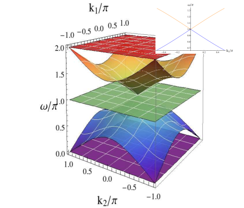
Figure 1: (Main Figure): Dispersion relation sketch around the diabolic point. The value of $\omega/\pi$ is plotted for the different sheets (i.e., different eigenvalues). The middle (flat) surface corresponds to $\omega_{k}^{(3)}=\pi$, the surface with values ranging from $1$ to $2$ corresponds to $\omega_{k}^{(1)}$. The bottom plane is associated with $\omega_{k}^{(4)}$ and the surface with values ranging from $0$ to $1$ corresponds to $\omega_{k}^{(2)}$. (Inset): Detail of $\omega_{k}^{(1)}$ and $\omega_{k}^{(2)}$ around the origin (orange and blue curves, respectively) for $k_{2}=0$ as a function of $k_{1}$, showing the intersection at the diabolical point.

For the sake of later use we note that the frequency $\Omega_{\mathbf{k}}$ reads, close to the diabolical point $\mathbf{k}=0$,

$$\Omega_{\mathbf{k}}\simeq\frac{k}{\sqrt{2}}-\frac{k^{3}\cos\left(2\theta\right)}{48\sqrt{2}}+O\left(k^{5}\right),$$ (52)

where $\mathbf{k}=k\left(\cos\theta,\sin\theta\right)$. This means that, very close to the diabolical point, the frequency $\Omega_{\mathbf{k}}$ actually has a conical dependence on the wavenumber. Later we will understand the consequences of the existence of these points.

The fact that $\omega_{\mathbf{k}}^{\left(s=3,4\right)}$ are constant causes that $\left|\psi_{\mathbf{x},t}^{\left(s=3,4\right)}\right\rangle$, see (23), do not have a wave character; only $\left|\psi_{\mathbf{x},t}^{\left(s=1,2\right)}\right\rangle$ are true waves. Hence propagation in the 2D Grover walk occurs only if the initial condition projects onto subspaces $1$ or $2$; otherwise the walker remains localized. This explains why strong localization in the 2D Grover map is usually observed, as first noted in Ref. Inui04 . All this can be put more formally in terms of the group velocity $\mathbf{v}_{\mathrm{g}}\left(\mathbf{k}\right)$ of the waves in the system, given by the gradient (in $\mathbf{k}$) of the wave frequency. The group velocity, as in any linear wave system, has the meaning of velocity at which an extended wave packet, centered in $\mathbf{k}$-space around some value $\mathbf{k}_{0}$, moves (there are other effects affecting extended wavepackets which we analyze below). In our case $\omega_{\mathbf{k}}^{\left(s=3,4\right)}$ are constant, hence their gradient is null: these eigenvalues entail no motion. On the contrary $\omega_{\mathbf{k}}^{\left(s=1,2\right)}$ depend on $\mathbf{k}$ (50,51) and then define non null group velocities:

$$\mathbf{v}_{\mathrm{g}}^{\left(1,2\right)}\left(\mathbf{k}\right)=\pm\nabla_{\mathbf{k}}\Omega_{\mathbf{k}},$$ (53)

where the plus and minus signs stand for $s=1,2$, respectively. Using (51) these velocities become

$$\mathbf{v}_{\mathrm{g}}^{\left(1,2\right)}\left(\mathbf{k}\right)=\pm\frac{(\sin{k_{1}},\sin{k_{2}})}{\sqrt{4-(\cos{k_{1}}+\cos{k_{2}})^{2}}}.$$ (54)

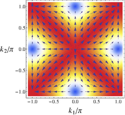
Figure 2: Vector plot of the group velocity (shown as arrows), superimposed to a density plot of the velocity modulus Eq. (51).

Hence the maximum group velocity modulus in the 2D Grover walk is $\frac{1}{\sqrt{2}}$, as can be easily checked and is obtained, in particular, along the diagonals $k_{2}=\pm k_{1}$. This is the maximum speed at which any feature of the QW can propagate. Figure 2 displays a vector plot of $\mathbf{v}_{\mathrm{g}}^{\left(1,2\right)}\left(\mathbf{k}\right)$ where a number of interesting points (in $\mathbf{k}$ space) is revealed: On the one hand there are points of null group velocity, located at $\mathbf{k}=\left(0,\pm\pi\right)$ and at $\mathbf{k}=\left(\pm\pi,0\right)$, in correspondence with the saddle points observed in Fig. 1. On the other hand there are five singular points at $\mathbf{k}=\left(0,0\right)$ as well as at the four corners. These points are singular because the group velocity is undefined at them (they look like sources or sinks). We note that these points coincide with the diabolical points in Fig. 1.

We find it worth mentioning that in two–dimensional QWs with coin operators other that the Grover, diabolical points are also found, as we have checked by using the DFT coin Mackay that displays several conical intersections. In this case of the DFT coin none of the four leaves of the dispersion relation is constant. We mention too that a behavior very similar to that of the 2D Grover walk is found in the Alternate QW Roldan12 , except for the fact that in this last case there are no constant surfaces in the dispersion relation (and hence no localization phenomena).

IV.2 Eigenvectors

The eigenvectors of the 2D Grover walk matrix (49) are given by Watabe . Use of these eigenvalues in (23) allows finally to compute the state of the system at any time.

Whenever $\mathbf{k}$ is not close to a diabolical point these eigenvectors vary smoothly around $\mathbf{k}$. Here we just want to study the behavior of the eigenvectors close to the diabolical point at $\mathbf{k}=\mathbf{k}_{\mathrm{D}}\equiv\left(0,0\right)$ –at the corners the conclusions are similar. We find it convenient to use polar coordinates $\left(k_{1},k_{2}\right)=\left(k\cos\theta,k\sin\theta\right)$. Performing the limit for $k\rightarrow 0$ we find

$$\phi_{\mathbf{k}}^{\left(1\right)} =\frac{1}{2\sqrt{2}}\left(\begin{array}[]{c}1+\sqrt{2}\cos\theta\\ 1-\sqrt{2}\cos\theta\\ -1-\sqrt{2}\sin\theta\\ -1+\sqrt{2}\sin\theta\end{array}\right),$$ (59)

$$\phi_{\mathbf{k}}^{\left(2\right)} =\frac{1}{2\sqrt{2}}\left(\begin{array}[]{c}1-\sqrt{2}\cos\theta\\ 1+\sqrt{2}\cos\theta\\ -1+\sqrt{2}\sin\theta\\ -1-\sqrt{2}\sin\theta\end{array}\right),$$ (64)

$$\phi_{\mathbf{k}}^{\left(3\right)} =\frac{1}{\sqrt{2}}\left(\begin{array}[]{c}\sin\theta\\ -\sin\theta\\ \cos\theta\\ -\cos\theta\end{array}\right),\ \ \phi_{\mathbf{k}}^{\left(4\right)}=\frac{1}{2}\left(\begin{array}[]{c}1\\ 1\\ 1\\ 1\end{array}\right).$$ (73)

Hence, close to the diabolical point $\mathbf{k}_{\mathrm{D}}$, there are three eigenvectors, corresponding to $s=1,2,3$, displaying a strong azimuthal dependence, while $\phi_{\mathbf{k}}^{\left(4\right)}$ is constant around $\mathbf{k}_{\mathrm{D}}$ (its variations are smooth and hence tend to zero as $\mathbf{k}\rightarrow\mathbf{k}_{\mathrm{D}}$). Thus, even if only $\phi_{\mathbf{k}}^{\left(1\right)}$ and $\phi_{\mathbf{k}}^{\left(2\right)}$ participate in the conical intersection and define the diabolical point, $\phi_{\mathbf{k}}^{\left(3\right)}$ is also affected by this feature because it is associated with eigenvalue $\lambda_{\mathbf{k}}^{\left(3\right)}=-1$, which is degenerate with $\lambda_{\mathbf{k}_{\mathrm{D}}}^{\left(s=1,2\right)}$. The fact that the diabolical point is singular is easy to understand: depending on the direction we approach to it the eigenvectors of the problem are different.

Just at the diabolical point $\lambda_{\mathbf{k}}^{\left(s=1,2,3\right)}=-1$ and hence there is a 3D eigensubspace formed by all vectors orthogonal to the fourth eigenvector, namely $\phi_{\mathbf{k}_{\mathrm{D}}}^{\left(4\right)}=\frac{1}{2}\operatorname{col}\left(1,1,1,1\right)$, which is equal to $\phi_{\mathbf{k}}^{\left(4\right)}$: see (73). A sensible choice for these eigenvectors follows from noting that $\phi_{\mathbf{k}}^{\left(1\right)}+\phi_{\mathbf{k}}^{\left(2\right)}$ in (73) is independent of the azimuth and is orthogonal to $\phi_{\mathbf{k}}^{\left(4\right)}$. Hence one of the basis elements for this 3D degenerate subspace can chosen as

$$\phi_{{}_{\mathrm{D}}}=\frac{\phi_{\mathbf{k}}^{\left(1\right)}+\phi_{\mathbf{k}}^{\left(2\right)}}{\sqrt{2}}=\frac{1}{2}\operatorname{col}\left(1,1,-1,-1\right),$$ (74)

which has the outstanding property of being the single vector that projects, close to the diabolical point $\mathbf{k}_{\mathrm{D}}$, only onto $\phi_{\mathbf{k}}^{\left(s=1,2\right)}$, i.e. onto the eigenspaces of the diabolo. As for the other two eigenvectors we just impose their orthogonality with $\phi_{{}_{\mathrm{D}}}$ and $\phi_{\mathbf{k}_{\mathrm{D}}}^{\left(4\right)}$ and we choose them arbitrarily as

$$\phi_{{}_{\mathrm{D}}}^{\prime}=\frac{1}{\sqrt{2}}\operatorname{col}\left(1,-1,0,0\right),\ \ \phi_{{}_{\mathrm{D}}}^{\prime\prime}=\frac{1}{\sqrt{2}}\operatorname{col}\left(0,0,-1,1\right).$$ (75)

Note that we are using a “primed” notation instead of keeping the notation with the label $s$, except for $s=4$, because none of these eigenvectors keeps being an eigenvector for $\mathbf{k}\neq\mathbf{k}_{\mathrm{D}}$ (only for special directions $\theta$) and hence there is no sense in attaching any of these eigenvectors to a particular sheet of the dispersion relation. To conclude we list the projections of these eigenvectors onto the eigenvectors (73) in the neighborhood of $\mathbf{k}_{\mathrm{D}}$:

$$\begin{array}[]{ll}\langle\phi_{{}_{\mathrm{D}}}\mid\phi_{\mathbf{k}}^{\left(1\right)}\rangle=\langle\phi_{{}_{\mathrm{D}}}\mid\phi_{\mathbf{k}}^{\left(2\right)}\rangle=\frac{1}{\sqrt{2}},&\langle\phi_{{}_{\mathrm{D}}}\mid\phi_{\mathbf{k}}^{\left(3\right)}\rangle=0,\\ \langle\phi_{{}_{\mathrm{D}}}^{\prime}\mid\phi_{\mathbf{k}}^{\left(1\right)}\rangle=-\langle\phi_{{}_{\mathrm{D}}}^{\prime}\mid\phi_{\mathbf{k}}^{\left(2\right)}\rangle=\frac{\cos\theta}{\sqrt{2}},&\langle\phi_{{}_{\mathrm{D}}}^{\prime}\mid\phi_{\mathbf{k}}^{\left(3\right)}\rangle=-\sin\theta,\\ \langle\phi_{{}_{\mathrm{D}}}^{\prime\prime}\mid\phi_{\mathbf{k}}^{\left(1\right)}\rangle=-\langle\phi_{{}_{\mathrm{D}}}^{\prime\prime}\mid\phi_{\mathbf{k}}^{\left(2\right)}\rangle=\frac{\sin\theta}{\sqrt{2}},&\langle\phi_{{}_{\mathrm{D}}}^{\prime\prime}\mid\phi_{\mathbf{k}}^{\left(3\right)}\rangle=\cos\theta,\end{array}$$ (76)

and $\left\langle\phi_{{}_{\mathrm{D}}}\right.\left|\phi_{\mathbf{k}}^{\left(4\right)}\right\rangle=\left\langle\phi_{{}_{\mathrm{D}}}^{\prime}\right.\left|\phi_{\mathbf{k}}^{\left(4\right)}\right\rangle=\left\langle\phi_{{}_{\mathrm{D}}}^{\prime\prime}\right.\left|\phi_{\mathbf{k}}^{\left(4\right)}\right\rangle=0$. All this has strong consequences on the QW dynamics near $\mathbf{k}_{\mathrm{D}}$ as we will show below.

IV.3 Continuous wave equations

In order to illustrate how the evolution of the QW can be controlled via an appropriate choice of the initial conditions, we will show some results obtained numerically from the evolution of the 2D quantum walk with the Grover operator. Unless otherwise specified, the initial profile in position space is a Gaussian centered at the origin with cylindrical symmetry (independent of $\alpha$ or $\eta$ ):

$$\psi_{\mathbf{x},0}=\mathcal{N}e^{i\mathbf{k}_{0}\cdot\mathbf{x}}e^{-\frac{x_{1}^{2}+x_{2}^{2}}{2\sigma^{2}}},$$ (77)

with $\mathbf{x}=(x_{1},x_{2})$, which implies that in the continuous limit we also have a Gaussian, in momentum space, centered at $\mathbf{k}_{0}=(k_{1},k_{2})$. Here, $\mathcal{N}$ is a constant that guarantees the normalization of the state. In the numerics, we have taken a sufficiently large value $\sigma=50$ for the Gaussian, so as to make it possible the connection with the continuous limit, although we will also discuss the situation for smaller values of $\sigma$ in order to show the robustness of the results.

Let us first consider a simple case having $k_{1}=k_{2}=\pi/2$, with an initial coin state $\frac{1}{\sqrt{2}}(\mid\phi_{\mathbf{k}_{0}}^{(1)}\rangle+\mid\phi_{\mathbf{k}_{0}}^{(2)}\rangle)$, where $\mid\phi_{\mathbf{k}_{0}}^{(1)}\rangle=\frac{1}{\sqrt{2}}\operatorname{col}\left(1,0,-1,0\right)$ and $\mid\phi_{\mathbf{k}_{0}}^{(2)}\rangle=\frac{1}{\sqrt{2}}\operatorname{col}\left(0,1,0,-1\right)$ that projects on the $s=1$ and $s=2$ branches with equal weights. The group velocity is given by $\mathbf{v}_{\mathrm{g}}^{\left(s\right)}\left(\mathbf{k}_{0}\right)=\pm(\frac{1}{2},\frac{1}{2})$, respectively for $s=1,2$, implying that the original Gaussian will split into two pieces that will move along the diagonal of the lattice in opposite directions, as shown in Fig. 3. It must be noticed that, since the second derivatives vanish at this point ($\varpi_{ij}=0)$, the Gaussian distribution moves with no appreciable distortion. On the right bottom panel of this figure, we show the result for $\sigma=5$ and we observe that, in this case, the results obtained for large $\sigma$ are very robust even for such a low value of $\sigma$.

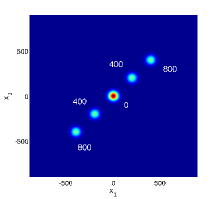
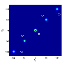
Figure 3: (Top panel): Probability distribution as a function of the dimensionless $(x_{1},x_{2})$ position. The initial condition is given by $\frac{1}{\sqrt{2}}(\mid\phi_{\mathbf{k}_{0}}^{(1)}\rangle+\mid\phi_{\mathbf{k}_{0}}^{(2)}\rangle)$ and $k_{1}=k_{2}=\pi/2$.. The distribution is shown for three times t=0, 400, 800 respectively. (Bottom panel): Top view of the previous figure, both for $\sigma=50$ (left) and $\sigma=5$ (right). The numbers indicate, in each case, the value of time for different snapshots.

However, if we choose an initial value $\mathbf{k}_{0}$ close to the origin, then the second derivatives take a large value, with the consequence that now the two pieces experience a considerable distortion along the line perpendicular to the line of motion, as can be seen from Fig. 4, where $k_{1}=k_{2}=0.01\pi$, implying a curvature $\varpi_{ij}\simeq 7.96$ in the perpendicular direction.

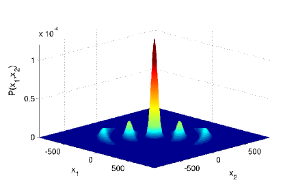
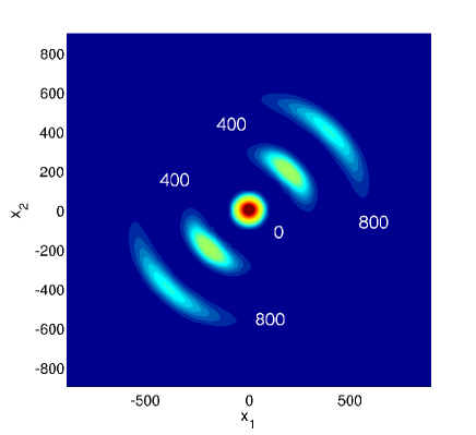
Figure 4: (Top panel): Probability distribution as a function of the dimensionless $(x_{1},x_{2})$ position. The initial condition is given by $\frac{1}{\sqrt{2}}(\mid\phi_{\mathbf{k}_{0}}^{(1)}\rangle+\mid\phi_{\mathbf{k}_{0}}^{(2)}\rangle)$ and $k_{1}=k_{2}=0.01\pi$. The distribution is shown for three times t=0, 400, 800 respectively. (Bottom panel): Top view of the previous figure, showing the value of the corresponding time steps.

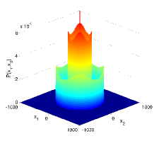
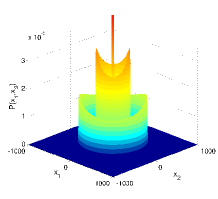
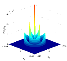
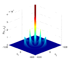
Figure 5: Same as Fig. 4, corresponding to four different values of $\sigma$. From left to right and from top to bottom: $\sigma=5$, $\sigma=10$, $\sigma=20$ and $\sigma=30$, respectively. The initial condition is given by $\frac{1}{\sqrt{2}}(\mid\phi_{\mathbf{k}_{0}}^{(1)}\rangle+\mid\phi_{\mathbf{k}_{0}}^{(2)}\rangle)$ and $k_{1}=k_{2}=0.01\pi$.

In this case, at variance with the case considered in Fig. 3, we have to face a peculiar situation, as the distribution is now peaked around a value close to the diabolical point $\mathbf{k}_{D}=\left(0,0\right)$. As far as the initial distribution does not contain this point with a significant probability (i.e., for a large value of $\sigma$), the behavior will be as described above. However, if $\sigma$ decreases below a certain limit, the evolution is dominated by the singular behavior of the diabolic point (to be studied in detail in the next subsection). This transition is clearly observed in Fig. 5, where the resulting evolution is depicted as $\sigma$ is increased from $\sigma=5$ to $\sigma=30$, the latter subpanel already showing a close resemblance with the result in Fig. 4. Distributions initially centered around non-singular points, however, are much more robust against a smaller $\sigma$, as previously shown in Fig. 3.

A completely different situation arises when $\mathbf{k}_{0}$ corresponds to one of the saddle points (such as the one located at $\mathbf{k}_{sp}=\left(0,\pi\right)$). As the group velocity vanishes at that point, i.e., $\mathbf{v}_{g}^{\left(1,2\right)}\left(\mathbf{k}_{0}\right)=\left(0,0\right)$, the center of the probability distribution is expected to remain at rest but will spread in time analogously to diffracting optical waves, as Eq. (37) reduces to the paraxial wave equation of optical diffraction Goodman . In our case, by considering $s=1$ as the initial coin state, one finds $\varpi_{11}=-1/2,\varpi_{12}=\varpi_{21}=0,\varpi_{22}=1/2.$ Therefore, Eq. (37) becomes

$$\mathrm{i}\frac{\partial A^{\left(1\right)}\left(\mathbf{X},t\right)}{\partial t}=-\frac{1}{4}\frac{\partial^{2}A^{\left(1\right)}}{\partial X_{1}^{2}}+\frac{1}{4}\frac{\partial^{2}A^{\left(1\right)}}{\partial X_{2}^{2}}.$$ (78)

This wave equation is similar to that of paraxial optical diffraction Goodman , differing from it in that the sign of spatial derivatives are different for the two spatial directions. Hence this hyperbolic equation describes a situation in which there is diffraction in one direction and anti-diffraction in the other direction, as it happens in certain optical systems Kolpakov . This causes that the cylindrical symmetry proper of diffraction is replaced by a rectangular symmetry. Basing on the analogy with diffraction, it is possible to tailor the initial distribution in order to reach a desired asymptotic distribution as we already demonstrated in the one-dimensional QW German . Hence if we want to reach a final homogeneous (top hat) distribution, we must use an initial condition of the form Goodman ; German

$$\psi_{\mathbf{x},0}=\mathcal{N}e^{i\mathbf{k}_{0}\cdot\mathbf{x}}e^{-\frac{x_{1}^{2}+x_{2}^{2}}{2\sigma^{2}}}sinc\left(x_{1}/\sigma_{0}\right)\,\,sinc\left(x_{2}/\sigma_{0}\right),$$ (79)

with $sinc\left(x\right)=\sin\left(\pi x\right)/\pi x$ and $\sigma_{0}$ a constant that accounts for the width of the distribution. In Fig. 6 we observe the evolution of the Grover walk with the above initial condition and the initial coin $\left|\phi_{\mathbf{k_{0}},0}^{(1)}\right\rangle=\frac{1}{2}col\left(1+i,1+i,1-i,1-i\right)$, equal for all populated sites. The figure shows a final distribution that is quite homogeneous along most of its support, except in its outer borders, where it shows a smooth but rapid fall out (the ratio $\sigma/\sigma_{0}$ has been chosen to optimize the result German ). This is the expected result, but Fig. 6 also shows a central peak that has been cut for a better display, the height of this central peak being quite large (around $1.5\cdot 10^{-5}$ ) as compared to the plateau (around $4\cdot 10^{-7}$). The existence of that central peak is a consequence of the common initial coin $\left|\phi_{\mathbf{k_{0}},0}\right\rangle$. This coin state guarantees that the initial distribution projects just onto the relevant branch of the dispersion relation at its central spatial frequency but, as the width of the distribution is finite, for the larger values of $\left|\mathbf{k}-\mathbf{k}_{0}\right|$ it will provide a non–negligible projection onto the static branches of the dispersion relation and the localized part of these projections are what we see as a central peak in Fig. 6.

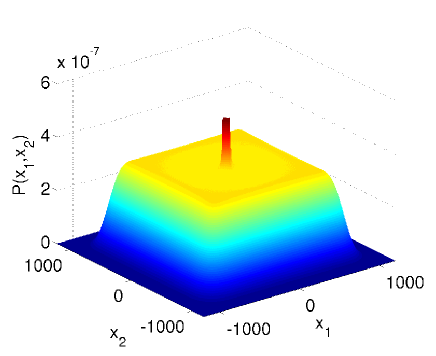
Figure 6: Probability distribution as a function of the dimensionless $(x_{1},x_{2})$ position at time t=9000, for initial conditions at the saddle point $\mathbf{k}_{0}=(0,\pi)$. The coin initial state is $\mid\phi_{\mathbf{k}_{0}}^{(1)}\rangle=\frac{1}{2}\operatorname{col}\left(1+i,1+i,1-i,1-i\right)$, and the starting space distribution as given by Eq. (79). We have taken a value $\sigma_{0}=15$ for this simulation. The central peak has been cut for a better display of the rest of the features.

IV.4 Dynamics at the diabolical points

In this case $N=2$, $\mathrm{d}^{N}\Omega=\mathrm{d}\theta$, with $\theta$ the azimuth, and

$$\left|\mathbf{E}_{\mathbf{x}}^{\left(s\right)}\left(k\right)\right\rangle=\int_{0}^{2\pi}\mathrm{d}\theta\exp\left(\mathrm{i}\mathbf{k}\cdot\mathbf{x}\right)\langle\phi_{\mathbf{k}_{\mathrm{D}}+\mathbf{k}}^{\left(s\right)}\mid\Xi\rangle\mid\phi_{\mathbf{k}_{\mathrm{D}}+\mathbf{k}}^{\left(s\right)}\rangle.$$ (80)

We remind that here $\left|\Xi\right\rangle$ is assumed to project just onto $\left|\phi_{\mathbf{k}_{\mathrm{D}}+\mathbf{k}}^{\left(s=1,2\right)}\right\rangle$. This means that $\left|\Xi\right\rangle$ coincides with $\left|\phi_{\mathrm{D}}\right\rangle$, see (74). According to the projections (76) and to the vectors (73) we can write, in matrix form,

$$\mathbf{E}_{\mathbf{x}}^{\left(s\right)}\left(k\right)=\frac{1}{4}\int_{0}^{2\pi}\mathrm{d}\theta\exp\left(\mathrm{i}\mathbf{k}\cdot\mathbf{x}\right)\left(\begin{array}[]{c}1\pm\sqrt{2}\cos\theta\\ 1\mp\sqrt{2}\cos\theta\\ -1\mp\sqrt{2}\sin\theta\\ -1\pm\sqrt{2}\sin\theta\end{array}\right),$$ (81)

where the upper (lower) sign in $\pm$ or $\mp$ corresponds to $s=1(2)$, respectively, and we remind that $\mathbf{k}=\left(k\cos\theta,k\sin\theta\right)$. Upon writing $\mathbf{k}\cdot\mathbf{x}=kx\cos\left(\theta-\varphi\right)$, where $\mathbf{x}=x\left(\cos\varphi,\sin\varphi\right)$ and performing the integral we arrive to

$$\mathbf{E}_{\mathbf{x}}^{\left(s\right)}\left(k\right)=\frac{\pi}{2}\left(\begin{array}[]{c}J_{0}\left(kx\right)\pm\mathrm{i}\sqrt{2}J_{1}\left(kx\right)\cos\varphi\\ J_{0}\left(kx\right)\mp\mathrm{i}\sqrt{2}J_{1}\left(kx\right)\cos\varphi\\ -J_{0}\left(kx\right)\mp\mathrm{i}\sqrt{2}J_{1}\left(kx\right)\sin\varphi\\ -J_{0}\left(kx\right)\pm\mathrm{i}\sqrt{2}J_{1}\left(kx\right)\sin\varphi\end{array}\right),$$ (82)

where $J_{n}$ are the Bessel functions of the first kind of order $n$. Using this result in (47) we get, in matrix form,

$$\mathbf{F}_{\mathbf{x},t}^{\left(s\right)}=\left(2\pi\right)^{-2}\int\mathrm{d}k\exp\left(\mp\mathrm{i}kct\right)k\tilde{F}_{k}\mathbf{E}_{\mathbf{x}}^{\left(s\right)}\left(k\right).$$ (83)

Let us compute the probability of finding the walker at some point, regardless the coin state, as given by (6), (22), (43) and (83). After simple algebra we obtain

$$P_{\mathbf{x},t}=\sum_{s,s^{\prime}}\left[\mathbf{F}_{\mathbf{x},t}^{\left(s\right)}\right]^{{\dagger}}\cdot\mathbf{F}_{\mathbf{x},t}^{\left(s^{\prime}\right)}=\left[p_{\mathbf{x},t}^{\left(0\right)}\right]^{2}+\left[p_{\mathbf{x},t}^{\left(1\right)}\right]^{2},$$ (84)

where

$$p_{\mathbf{x},t}^{\left(0\right)} =\left(2\pi\right)^{-1}\int_{0}^{\infty}\mathrm{d}k\cos\left(kct\right)J_{0}\left(kx\right)k\tilde{F}_{k},$$ (85)

$$p_{\mathbf{x},t}^{\left(1\right)} =\left(2\pi\right)^{-1}\int_{0}^{\infty}\mathrm{d}k\sin\left(kct\right)J_{1}\left(kx\right)k\tilde{F}_{k},$$ (86)

are amplitude probabilities. We see that the spatial dependence of the probability amplitude on the azimuth $\varphi$ in (83,82) disappears when looking at the full probability $P_{\mathbf{x},t}$. This means that a coin-sensitive measurement of the probability should display angular features.

As a summary of what we know up to here about the neighborhood of the diabolical point, we can say that when the initial coin $\left|\Xi\right\rangle$ coincides with $\left|\phi_{\mathrm{D}}\right\rangle$, see (74), we predict (i) no localization and, (ii) when the initial wave packet $F_{\mathbf{x},0}$ is radially symmetric (it only depends on $x=\left|\mathbf{x}\right|$), an evolution of the probability $P_{\mathbf{x},t}$ that keeps the radial symmetry along time, according to (84,85,86).

Equations (85) and (86) describe the evolution of the probability of an initial wave packet centered at a diabolical point and with radial symmetry. The actual probability $P_{\mathbf{x},t}$ can be computed from them numerically, but little can be said in general. In order to gain some insight we consider next the relevant long time limit, which turns out to be analytically tractable. First of all it is convenient to scale the radial wavenumber $k$ to the (loosely defined) width of the initial state in real space, $F_{\mathbf{x},0}$, which we denote by $\sigma$. Accordingly we define $\kappa=\sigma k$ so that (85) and (86) become

$$p_{\mathbf{x},t}^{\left(0\right)} =\left(2\pi\sigma^{2}\right)^{-1}\int_{0}^{\infty}\mathrm{d}\kappa\cos\left(\frac{ct}{\sigma}\kappa\right)J_{0}\left(\frac{x}{\sigma}\kappa\right)\kappa\tilde{f}_{\kappa},$$ (87)

$$p_{\mathbf{x},t}^{\left(1\right)} =\left(2\pi\sigma^{2}\right)^{-1}\int_{0}^{\infty}\mathrm{d}\kappa\sin\left(\frac{ct}{\sigma}\kappa\right)J_{1}\left(\frac{x}{\sigma}\kappa\right)\kappa\tilde{f}_{\kappa},$$ (88)

where $\tilde{f}_{\kappa}=\tilde{F}_{k=\kappa/\sigma}$ is non null only for $\kappa\lesssim 1$. Hence when $ct\gg\sigma$, $\cos\left(\frac{ct}{\sigma}\kappa\right)$ and $\sin\left(\frac{ct}{\sigma}\kappa\right)$ are strongly oscillating functions of $\kappa$, around zero, what would make $p_{\mathbf{x},t}^{\left(0,1\right)}$ to vanish. However in the integrals defining such amplitude probabilities other oscillating functions, $J_{0}\left(\frac{x}{\sigma}\kappa\right)$ and $J_{1}\left(\frac{x}{\sigma}\kappa\right)$, appear. Thus it can be expected that when the oscillations of the latter and the ones of the former are partially in phase, a non null value of the integrals is got. According to the asymptotic behavior of $J_{n}\left(z\right)$ at large $z$, $J_{n}\left(z\right)\approx\sqrt{2/\pi z}\cos\left(z-n\pi/2-\pi/4\right)$ for $z\gg\left|n^{2}-1/4\right|$ Bessel , this partial phase matching occurs when $x\approx ct$, which is expected from physical considerations. Hence we are led to consider the limit $x=ct+\sigma\xi$, with $ct\gg\sigma$, where $\xi$ is the scaled radial offset with respect to $ct$, in which case (87) and (88), after expressing the products of trigonometric functions as sums, become

$$p_{\mathbf{x},t}^{\left(0\right)} =p_{\mathbf{x},t}^{\left(1\right)}$$

$$\approx\left(2\pi\sigma^{2}\right)^{-1}\sqrt{\frac{\sigma}{2\pi ct}}\int_{0}^{\infty}\mathrm{d}\kappa\sin\left(\kappa\xi+\pi/4\right)\sqrt{\kappa}\tilde{f}_{\kappa}$$

$$=\left(2\pi\right)^{-1}/\sqrt{2\pi ct}\int_{0}^{\infty}\mathrm{d}k\sin\left(k\sigma\xi+\pi/4\right)\sqrt{k}\tilde{F}_{k},$$ (89)

to the leading order, where the approximation follows from disregarding highly oscillating terms. As an application of this result we consider next the Gaussian case $\tilde{F}_{k}=2\sigma\sqrt{\pi}\exp\left(-\frac{1}{2}\sigma^{2}k^{2}\right)$, where $\sigma$ is the standard deviation of the initial probability in real space, Eq. (77). We readily obtain

$$p_{\mathbf{x},t}^{\left(0\right)} =p_{\mathbf{x},t}^{\left(1\right)}=\frac{1}{8\sqrt{\sigma ct}}e^{-\xi^{2}/4}$$

$$\times\left\{\xi\sqrt{\left|\xi\right|}\left[I_{-1/4}\left(\xi^{2}/4\right)-I_{3/4}\left(\xi^{2}/4\right)\right]\right.$$

$$+\left.\frac{\xi^{2}I_{5/4}\left(\xi^{2}/4\right)-\left(\xi^{2}-2\right)I_{1/4}\left(\xi^{2}/4\right)}{\sqrt{\left|\xi\right|}}\right\},$$ (90)

where $\xi=\frac{x-ct}{\sigma}$ and $I_{n}$ is the modified Bessel function of the first kind of order $n$. The total probability $P_{\mathbf{x},t}\equiv P(\xi)$ follows from using (90) in (84), from which we observe that the initial width $\sigma$ acts only as a scale factor for the height and shape of the probability at long times ($ct\gg\sigma$). A plot of the probability can be seen in Fig. 8, where two unequal spikes, whose maxima are located at $\xi=-1.74623$ and at $\xi=0.550855$, separated by a zero at $\xi=-0.765951$, are apparent. We remind that $x=ct+\sigma\xi$ is a radial coordinate, hence these maxima correspond to two concentric rings separated by a dark ring. The situation is fully analogous to the so-called “Poggendorff rings” appearing in the paraxial propagation of a beam incident along an optic axis of a biaxial crystal, a situation in which a conical intersection (a diabolical point) is present. Remarkably the result we have obtained for $P_{\mathbf{x},t}$ fully coincides with that described in Berry2 whose Fig. 7 is to be compared to our Fig. 8.

As an example that illustrates the above features, we have studied the evolution of a state of the form Eq. (77) for the diabolic point $\mathbf{k}_{\mathrm{D}}=(0,0)$, and a coin state as defined in Eq. (74). As seen from Fig. 7, the probability distribution keeps its cylindrical symmetry while it expands in position. It can also be seen from this figure that the general features remain valid for a wider distribution (in $k$ space) corresponding to $\sigma=5$, even if the distribution in spatial coordinates is narrower for a given time step. The Poggendorff rings can be appreciated in Fig. 8, which shows a radial cut of the previous figure. We also plot for comparison our analytical result, as obtained form Eqs. (84) and (90) , which shows a good agreement with the (exact) numerical result, as can be seen from this figure.

All these features crucially depend on the choice of the coin initial conditions, as clearly observed when these conditions are chosen differently. As an example, we show in Fig. 9 the evolution after 200 time steps, of the probability distribution when we start from a state, also centered around the diabolic point, but the vector coin is now $\left|\phi_{\mathbf{k}_{\mathrm{D}}}^{\left(2\right)}\right\rangle$ with $\theta=\pi/2$. Most of the probability is directed along the positive $x_{2}$ axis, which corresponds to the choice of $\theta$. In fact, by changing the value of this parameter one can, at will, obtain a chosen direction for propagation.

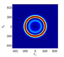
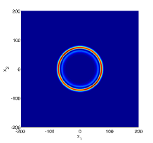
Figure 7: (Top panel): Probability distribution as a function of the dimensionless $(x_{1},x_{2})$ position, at time $t=400$. The initial condition is given by Eq. (74) around the diabolic point $\mathbf{k}_{\mathrm{D}}=(0,0)$, with $\sigma=50$. (Bottom panel): Top view of the previous figure with $\sigma=50$ (left) and $\sigma=5$ (right), but now at time $t=100$.

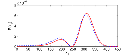
Figure 8: Radial cut, with $x_{2}=0$, for the top panel of Fig. 7 (blue, dotted curve), showing the Poggendorff rings (see the text for explanation). Also shown for comparison is our analytical result, as obtained form Eqs. (84) and (90) (solid, red curve).

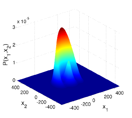
Figure 9: Probability distribution as a function of the dimensionless $(x_{1},x_{2})$ position, at time $t=200$. The initial condition is given by $\left|\phi_{\mathbf{k}_{\mathrm{D}}}^{\left(2\right)}\right\rangle$ around the diabolic point with $\theta=\pi/2$ .

V Application to the 3D Grover QW

In this section we briefly analyze the three–dimensional Grover QW in order to illustrate similarities and differences with the two–dimensional case. In 3D, the Grover-coin operator reads

$$C=\frac{1}{3}\left(\begin{array}[]{cccccc}-2&1&1&1&1&1\\ 1&-2&1&1&1&1\\ 1&1&-2&1&1&1\\ 1&1&1&-2&1&1\\ 1&1&1&1&-2&1\\ 1&1&1&1&1&-2\end{array}\right),$$ (91)

and the diagonalization of the corresponding matrix $C_{\mathbf{k}}$ (17), with $\mathbf{k}=(k_{1},k_{2},k_{3})$, yields six eigenvalues $\lambda_{\mathbf{k}}^{\left(s\right)}=\exp\left(-\mathrm{i}\omega_{\mathbf{k}}^{\left(s\right)}\right)$ with

$$\omega_{\mathbf{k}}^{\left(1,2\right)}=\pm\Omega_{\mathbf{k}}^{\left(+\right)},\text{ }\omega_{\mathbf{k}}^{\left(3,4\right)}=\pm\Omega_{\mathbf{k}}^{\left(-\right)},\ \omega_{\mathbf{k}}^{\left(5\right)}=0,\text{ }\omega_{\mathbf{k}}^{\left(6\right)}=\pi,$$ (92)

where

$$\cos\Omega_{\mathbf{k}}^{\left(\pm\right)} =-\frac{1}{3}\left[\sum_{i=1,2,3}\cos{k_{i}\pm}\right.$$

$$\left.\sqrt{\sum_{i=1,2,3}^{j>i}\left(\cos^{2}{k_{i}}-\cos{k_{i}\cos}k_{j}\right)}\right].$$ (93)

Remember that adding a multiple integer of $2\pi$ to any of the $\omega$’s does not change anything because time is discrete and runs in steps of $1$. This implies that $\omega=-\pi$ and $\omega=\pi$ represent the same frequency.

The graphical representation is more complicated in the 3D case: Plots of the dispersion relations (92) for particular values of $k_{3}$ and for particular values of $\omega$ are given in Figs. 10 and 11, respectively.

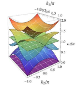
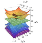
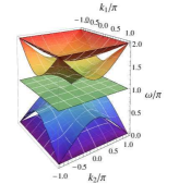
Figure 10: Representations of the Grover 3D six dispersion relation surfaces for $k_{3}=0$ (left), $\pi/2$ (center), and $\pi$ (right).

A large variety of propagation properties can be expected depending on the particular region in $k$-space that the initial distribution occupies. Notice the existence of two constant dispersion relations, $\omega_{\mathbf{k}}^{\left(5,6\right)}$, which will give rise to localization phenomena, as already discussed in the 2D case.

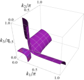
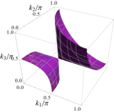
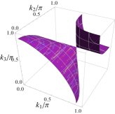
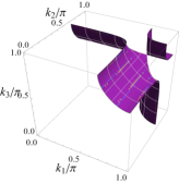
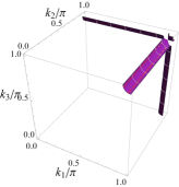
Figure 11: Representations of the Grover 3D isofrequency surfaces, as obtained from $\Omega_{\mathbf{k}}^{\left(+\right)}$ in the first octant of the Brillouin zone for $\omega=0.95\pi$ (a), $0.8\pi$ (b), $0.6\pi$ (c), $0.4\pi$ (d), $0.2\pi$ (e), and $0.05\pi$ (f). For $\omega=\pi$ the two dispersion relation coincides with the cube axes and the cube origin, whilst for $\omega=0$ they have migrated to the opposite side of the cube.

There exist several degeneracies in the above dispersion relations, appearing in the crossings of several dispersion curves. For $\omega=\pi$, there is a 5-fold degeneracy at $\mathbf{k}=\mathbf{0}$, where $\omega_{\mathbf{k}}^{\left(j\right)}=\pi$ for $j=1,2,3,4,6$. There is also a 3-fold degeneracy occurring when $\mathbf{k}$ takes the form $\mathbf{k}=\mathbf{k}_{||}\equiv k\mathbf{e}_{i}$, where $\mathbf{e}_{i}$ is one of the vectors of the canonical basis in $\mathbb{R}^{3}$(i.e., $\mathbf{k}_{||}$ has two null components and an arbitrary third component), where $\omega_{\mathbf{k}}^{\left(j\right)}=\pi$ for $j=1,2,6$. For $\omega=0$ these degeneracies migrate to the corners and borders, respectively, of the first Brillouin zone, see Fig. 11. The frequencies $\Omega_{\mathbf{k}}^{\left(\pm\right)}$, close to the degeneracies for $\omega=\pi$, read

$$\left.\cos\Omega_{\mathbf{k}}^{\left(\pm\right)}\right|_{\mathbf{k}=0} \simeq-1+\frac{1}{6}\left|\mathbf{k}\right|^{2}\mp$$

$$\frac{1}{6}\sqrt{\left|\mathbf{k}\right|^{4}-3\left(k_{x}^{2}k_{y}^{2}+k_{x}^{2}k_{z}^{2}+k_{y}^{2}k_{z}^{2}\right)}+O\left(k^{4}\right).$$ (94)

In the case that $\mathbf{k}$ takes the form $\mathbf{k}=\mathbf{k}_{||}\equiv k\mathbf{e}_{i}$, we obtain

$$\cos\Omega_{\mathbf{k}}^{\left(+\right)}=-1$$ (95)

$$\cos\Omega_{\mathbf{k}}^{\left(-\right)}=-\frac{1}{3}(1+2\cos k)$$ (96)

which shows the above-mentioned degeneracy.

We see that the point degeneracy occurring at $\mathbf{k}=0$, $\cos\Omega_{\mathbf{k}}^{\left(+\right)}=-1$, is not a true diabolical point because, for fixed frequency, the dispersion relation has not spherical symmetry (hence the dispersion relation surface is not a hyperdiabolo). This implies that the theory developed in Sec. III.B cannot be applied to this case. (We notice, however, that it can be applied when coins different to the Grover one are used as it occurs, for example, in the Alternate 3D QW, where true 3D diabolical points exist Roldan12 .)

Its not difficult to see that the group velocities

$$\mathbf{v}_{\mathrm{g}}^{\left(1,2,3,4\right)}\left(\mathbf{k}\right)=\pm\nabla_{\mathbf{k}}\Omega_{\mathbf{k}}^{\left(\pm\right)},$$ (97)

have now the expression

$$\left(\mathbf{v}_{\mathrm{g}}^{\left(1,2\right)}\left(\mathbf{k}\right)\right)_{i} =\mp\frac{(2\cos\Omega_{\mathbf{k}}^{\left(+\right)}+\sum_{j\neq i}\cos k_{j})\sin k_{i}}{2\left(3\cos\Omega_{\mathbf{k}}^{\left(+\right)}+\sum_{j}\cos k_{j}\right)\sin\Omega_{\mathbf{k}}^{\left(+\right)}},$$ (98)

$$\left(\mathbf{v}_{\mathrm{g}}^{\left(3,4\right)}\left(\mathbf{k}\right)\right) {}_{i}=\mp\frac{(2\cos\Omega_{\mathbf{k}}^{\left(-\right)}+\sum_{j\neq i}\cos k_{j})\sin k_{i}}{2\left(3\cos\Omega_{\mathbf{k}}^{\left(-\right)}+\sum_{j}\cos k_{j}\right)\sin\Omega_{\mathbf{k}}^{\left(-\right)}},$$ (99)

and $\mathbf{v}_{\mathrm{g}}^{\left(5,6\right)}\left(\mathbf{k}\right)=0$.

We see that the extrema of the dispersion relations for branches 1,2,3 and 4 giving points of null velocity (those for which a Schrödinger type equation is a priori well suited for extended initial conditions) occur, in particular, when all $\sin k_{i}=0$. At some of these points we find the just discussed degeneracies, hence at them a Schrödinger type equation is not appropriate. However, some of the points of null velocity do not correspond to degeneracies, in particular those $\mathbf{k}$ with two null components and the third one equal to $\pm\pi$. Consider, for example, the point $\mathbf{k}_{0}=\left(0,0,\pm\pi\right)$ at which $\Omega_{\mathbf{k}}^{\left(+\right)}$ presents degeneracies but not $\Omega_{\mathbf{k}}^{\left(-\right)}$, which takes the value $\Omega_{\mathbf{k}}^{\left(-\right)}=\arccos 1/3$. In order to particularize the wave equation (1) to this case we must calculate the nine coefficients

$$\ \varpi_{ij}^{\left(3,4\right)}=\pm\left.\partial^{2}\Omega_{\mathbf{k}}^{\left(-\right)}/\partial k_{i}\partial k_{j}\right|_{\mathbf{k}=\mathbf{k}_{0}},$$ (100)

which turn out to be $\varpi_{11}^{\left(3,4\right)}=\varpi_{22}^{\left(3,4\right)}=-\varpi_{33}^{\left(3,4\right)}/4=\mp 1/4\sqrt{2}$ the rest being zero. Hence the continuous description in this case is given by

$$\mathrm{i}\frac{\partial A^{\left(3,4\right)}}{\partial t}=\pm\frac{1}{8\sqrt{2}}\left(\frac{\partial^{2}}{\partial X_{1}^{2}}+\frac{\partial^{2}}{\partial X_{2}^{2}}-4\frac{\partial^{2}}{\partial X_{3}^{2}}\right)A^{\left(3,4\right)},$$ (101)

which exhibits an anisotropic diffraction (diffraction in the $\left(X_{1},X_{2}\right)$ plane and anti-diffraction, with a different coefficient, in the $X_{3}$ direction). For $\mathbf{k}_{0}=\left(\pi,0,0\right)$ and $\mathbf{k}_{0}=\left(0,\pi,0\right)$ the result is the same after making the changes $X_{1}\rightarrow X_{3}$ and $X_{2}\rightarrow X_{3}$, respectively. Eq. (101) can be solved via a Fourier transform method. For a starting Gaussian profile as given below, the solution will factorize in three one dimensional functions of the form

$$\frac{e^{-\frac{ix^{2}}{2t\varpi+2i\sigma^{2}}}}{\sqrt{\sigma^{2}-it\varpi}}$$ (102)

(except for an overall constant), where $\varpi$ is any of the coefficients $\varpi_{ij}$ that appear in Eq. (101), and $x$ represents one of the coordinates $X_{i}$ with $i=1,2,3$. This implies a characteristic time scale $t\sim\sigma^{2}/|\varpi|$ for the Gaussian to broaden.

We now show two examples that illustrate the above results. As in the 2D cases, we start with an initial condition (41) defined by a Gaussian shape

$$\psi_{\mathbf{x},0}=\mathcal{N}e^{i\mathbf{k}_{0}\cdot\mathbf{x}}e^{-\frac{x_{1}^{2}+x_{2}^{2}+x_{3}^{2}}{2\sigma^{2}}},$$ (103)

with $\mathcal{N}$ an appropriate constant defining the normalization, and $\left|\Xi\right\rangle$ a constant (position-independent) vector in the coin space, which is chosen to be one of the eigenvectors of the matrix $C_{\mathbf{\mathbf{k}}}$ (17) at the point $\mathbf{\mathbf{k}=k}_{0}$. We have not explored those cases where $\mathbf{k}_{0}$ lies at, or very close to, any of the degeneracies discussed above. The problem at these points seems to be much more involved than in the 2D case. For example, the extension of the eigenvectors obtained in Watabe to this case encounters a singular behavior at the axis (which are degeneracy lines). One needs to carefully take care of the appropriate limit as one approaches these lines, and perform a systematic study in order to find the relevant linear combinations providing a sensible time evolution. Such a study is beyond the scope of this paper.

We first start with a value $\mathbf{k}_{0}=(0.1,0.2,0.3)\pi$ that lies far from any degeneracy or points with zero group velocity. For $s=3$, the group velocity is $\mathbf{v}_{\mathrm{g}}^{\left(3\right)}\left(\mathbf{k}_{0}\right)=(-0.028,-0.232,-0.704)$. In Fig. 12 we show two different views corresponding to the evolved probability distribution.

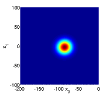
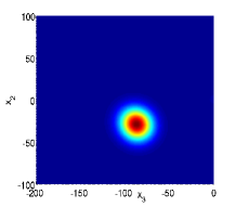
Figure 12: Top view of the probability distribution in position space on the $x_{2}=0$ plane (left) and on the $x_{1}=0$ plane (right) for a time step $t=125$. The initial distribution is given by Eqs. (41) and (103), with $\mathbf{k}_{0}=(0.1,0.2,0.3)\pi$ and $\left|\Xi\right\rangle$ the eigenvector of the coin operator corresponding to $s=3$.

Within the timescale displayed on this Figure, the initial Gaussian has not appreciably broaden, and we can instead observe the motion of the center of the wave packet according to what is expected from the group velocity. A somehow opposite behavior is observed if we choose a point giving a zero velocity, such as $\mathbf{k}_{0}=(0,0,\pi)$. As described above, we expect no motion of the center and a broadening which depends on the axis we choose. This broadening can be approximately described by Eq. (101) and, for the values of $\sigma$ we are assuming here, one needs to follow the time evolution during a considerably larger time scale. As a consequence, higher order effects neglected in deriving Eq. (101) may accumulate. In Fig. 13 we show two different radial cuts of the 3D probability distribution.

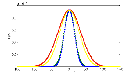
Figure 13: Two different radial cuts of the evolved probability distribution, represented by $P(r)$, where $r$ is the coordinate along the cut, at $t=1000$ when the initial distribution is a spherically symmetric Gaussian function with $\sigma=20$, with $\mathbf{k}_{0}=(0,0,\pi)$ and $\left|\Xi\right\rangle$ the eigenvector of the coin operator corresponding to $s=3$. The figure also shows for comparison the analytical result as obtained from Eq. (101). The curve with red symbols corresponds to a cut along the $x_{3}$ axis, to be compared with the analytical approximation (yellow curve). The curve with blue symbols is the plot for a cut along the $x_{3}$ axis, to be compared with the analytical approximation (green).

As observed from this Figure, the accumulated discrepancy between the exact numerical evolution and the approximated analytical Eq. (101) may depend on the spatial direction. However, given all these considerations, we see that our derived analytical result gives a reasonable description for the main features of the time evolution, even in 3D.

VI Conclusions

In this article we have formally solved the standard multidimensional QW, taking into account extended initial conditions of arbitrary shape and width. In the limit of large width, the continuous limit is particularly well suited and clearly reveals the wave essence of the walk. The use of the dispersion relations is the central argument behind this view as its analysis allows to get much insight into the propagation properties of the walk, even allowing for the tailoring of the initial distribution in order to reach a desired asymptotic distribution, as we have demonstrated. We must insist here in that our goal was not to obtain approximate solutions to the QW, thus quantifying their degree of accuracy, but rather to get qualitative insight into the long term solutions. The equations we have derived will be quite accurate for wide initial conditions, but the interesting point is that they provide a good qualitative description for relatively narrow initial distributions, specially far from degeneracies.

We have also shown that the two dimensional Grover QW exhibits a diabolical point in its dispersion relations, and have analyzed in detail the dynamics around this point, closely connecting the Grover walk with the phenomenon of conical refraction Berry2 ; Berry3 . In the three–dimensional Grover walk we have found other types of degeneracies whose influence on the dynamics we have not illustrated. The detailed study of the construction of the eigenvectors providing a clear qualitative interpretation turns out to be much more complicated in the 3D than in the 2D case, and we leave this extensive study for a future work.

We want to insist in that the asymptotic distributions found in the continuous limit, valid for large initial distributions, can be qualitatively reached for not very broad distributions, say $\sigma\sim 5$, and this should be easy to implement in systems such as the optical interferometers of Ref. Schreiber ; Schreiber12 . An exception to this general rule are those distributions which are peaked close to the diabolic point, since in this case a broad distribution will be dominated by the singular nature of that point.

As a final comment we would like to say, on the one hand, that the multidimensional QW can be viewed as a simulator of a large variety of linear differential equations depending on the particular region of the dispersion relation that governs the evolution of the initial wave–packet. On the other hand, we stress that continuous approximations to the QW must follow the dispersion relation if they are to be taken as good approximations.

References

- (1) Aharonov Y, Davidovich L, and Zagury N 1993 Phys. Rev. A 48 1687
- (2) Meyer D A 1996 J. Stat. Phys. 85 551
- (3) Watrous J 2001 Proc. STOC’01 (New York: ACM) pp 60
- (4) Nayak A and Vishwanath A 2000 (Preprint quant-ph/0010117)
- (5) Ambainis A 2003 Int. J. Quant. Inf. 1 507
- (6) Kempe J 2003 Contemp. Phys. 44 307
- (7) Kendon V 2006 Math. Struct. Comp. Sci. 17 1169
- (8) Kendon V 2006 Phil. Trans. R. Soc. A 364 3407
- (9) Konno N 2008 Quantum Walks in Quantum Potential Theory Lect. Notes Math. 1954, (ed. by U. Franz and M. Schürmann Springer)
- (10) Childs A M 2009 Phys. Rev. A 102 180501
- (11) Lovett N B, Cooper S, Everitt M, Trevers M, and Kendon V 2010 Phys. Rev. A 81 042330
- (12) Knight P L, Roldán E and Sipe J E 2004 J. Mod. Opt. 51 1761
- (13) de Valcárcel G J, Roldán E and Romanelli A 2010 New J. Phys. 12 123022
- (14) Flitney A P 2012 (Preprint arXiv:1209.2252)
- (15) Buerschaper O and Burnett K 2004 (Preprint quant-ph/0406039)
- (16) Wojcik A, Luczak T, Kurzynski P, Grudka A and Bednarska M 2004 Phys. Rev. Lett. 93 180601
- (17) Romanelli A, Auyuanet A, Siri R, Abal G and Donangelo R 2005 Physica A 352 409
- (18) Romanelli A 2012 Phys. Rev.A 85 012319
- (19) Kurzynski P and Wojcik A 2012 (Preprint arXiv:1208.1800)
- (20) Bouwmeester D, Marzoli I, Karman G P, Schleich W and Woerdman W 1999 Phys. Rev. A 61 013410
- (21) Knight P L, Roldán E, and Sipe J E 2003 Phys. Rev. A 68 020301(R)
- (22) Jeong H J, Paternostro M, Kim M S 2003 Phys. Rev. A 69 012310
- (23) Knight P L, Roldán E and Sipe J E 2003 Opt. Commun. 227 147; 2004 erratum 232 443
- (24) Roldán E and Soriano JC 2005 J. Mod. Opt. 52 2649
- (25) Do B, Stohler M L, Balasubramanian S, Elliot D S, Eash Ch, Fischbach E, Fischbach M A, Mills A and Zwickl B 2005 J. Opt. Soc. Am. 22 499
- (26) Bañuls M C, Navarrete C, Pérez A, Roldán E, and Soriano J C 2006 Phys. Rev. A 73 062304
- (27) Perets H B, Lahini Y, Pozzi F, Sorel M, Morandotti R and Silberberg Y 2008 Phys. Rev. Lett. 100 170506
- (28) Schreiber A, Cassemiro K N, Potoček V, Gábris A, Mosley P J, Andersson E, Jex I and Silberhorn Ch 2010 Phys. Rev. Lett. 104 050502
- (29) Dür W, Raussendorf R, Kendon V M and Briegel H-J 2002 Phys. Rev. A 66, 052319
- (30) Eckert K, Mompart J, Birkl G and Lewenstein M, 2005 Phys. Rev. A 72 012327
- (31) Chandrashekar C M and Laflamme R 2008 Phys. Rev. A 78 022314
- (32) Karski M, Förster L, Choi J -M, Steffen A, Alt W, Meschede D and Widera A 2009 Science 325 174
- (33) Travaglione B C and Milburn G J Phys. Rev. A 65 032310 (2002)
- (34) Schmitz H, Matjeschk R, Schneider Ch, Glueckert J, Enderlein M, Huber T and Schaetz T 2009 Phys. Rev. Lett. 103 090504
- (35) Zähringer F, Kirchmair G, Gerritsma R, Solano E, Blatt R and Roos C F 2010 Phys. Rev. Lett. 104 100503
- (36) Chandrashekar C M 2006 Phys. Rev. A 74 032307
- (37) Schreiber A, Gabris A, Rohde P P, Laiho K, Stefanak M, Potocek V, Hamilton C, Jex I and Silberhorn Ch 2012 Science 336 55
- (38) Reitzner D, Nagaj D, Buzek V 2011 Acta Phys. Slov. 61 603
- (39) Venegas-Andraca S E 2012, Quantum Inf. Proc. 11 1015-1106
- (40) Roldán E, Silva F, Di Franco C and de Valcárcel G J Phys. Rev. A 87 022336 (2013)
- (41) Kempf A and Portugal R 2009 Phys. Rev. A 79 052317
- (42) Stefanak M, Bedzekova I and Jex I 2012 Eur. J. Phys. D 66 5
- (43) Rohde P P, Schreiber A, Stefanak M, Jex I and Silberhorn Ch 2011 New. J. Phys. 13 013001
- (44) Machida E (Preprint arXiv:1207.3614)
- (45) Di Franco C, Mc Gettrick M, Machida T and Busch Th 2011 Phys. Rev. A 84 042337
- (46) Mackay T T D, Bartlett S, Stephenson L and Sanders B 2002 J. Phys. A: Math. Gen. 35 2745
- (47) Tregenna B Flanagan W, Maile R and Kendon V 2003 New. J. Phys. 5 83
- (48) Shenvi N, Kempe J, BirgittaWhaley K 2003 Phys. Rev. A 67 052307
- (49) Inui N, Konichi Y, Konno N 2004 Phys. Rev. A 69 052323
- (50) Carneiro I, Loo M, Xu X, Girerd M, Kendon V and Knight P L 2005 New J. Phys. 7 156
- (51) Oliveira A, Portugal R and Donangelo R 2006 Phys. Rev. A 74 012312
- (52) Omar Y, Paunkovic N, Sheridan L and Bose S 2006 Phys. Rev. A 74 042304
- (53) Adamczak W, Andrew K, Bergen L, et al 2007 Int. J. Quantum Inf. 5 781
- (54) Marquezino F, Portugal R, Abal G and Donangelo R 2008 Phys. Rev. A 77 042312
- (55) Venegas-Andraca S E 2008 Quantum Walks for Computer Scientists (Morgan and Claypool publishers)
- (56) Watabe K, Kobayashi N, Katori M and Konno N 2008 Phys. Rev. A 77 062331
- (57) Stefanák M, Kollar B, Kiss T and Jex I 2010 Phys. Scr. T140 014035
- (58) Stefanák M, Kollar B, Kiss T and Jex I 2008 Phys. Rev. A 78 032306
- (59) Berry M V and Wilkinson M 1984 Prox. R. Soc. Lond. 392 15
- (60) Berry M V 2004, J. Opt. A: Pure Appl. Opt. 6 289
- (61) Berry M V and Jeffrey M R 2007 Prog. Opt. 50 13
- (62) Hatsugai Y, Fukui T, and Aoki H 2007 (Preprint arXiv:cond-mat/0701431)
- (63) Bostwick A, Ohta T, McChesney J L, Emtsev K V, Seyller T, Horn K, and Rotenberg E 2007 New. J. Phys. 9 385
- (64) Ohta T, Bostwick A, McChesney J L, Seyller T, Horn K, and Rotenberg E 2007 Phys. Rev. Lett. 98 206802
- (65) Pletikosić I, Kralj M,1, Pervan P, Brako R, Coraux J, N’Diaye A T, Busse C, and Michely T 2009 Phys. Rev. Lett. 102 056808
- (66) Castro Neto A H, Guinea F, Peres N M R, Novoselov K S and Geim K S 2009 Rev. Mod. Phys. 81 109
- (67) Mead C A and Truhlar D G, 1979 J. Chem. Phys. 70 2284
- (68) Cederbaum L S, Friedman R, Ryaboy V M and Moiseyev N 2003 Phys. Rev. Lett. 90 013001
- (69) Zhang M, Hung H-h, Zhang Ch, and C Wu 2011 Phys. Rev. A 83 023615
- (70) Torrent D and Sánchez-Dehesa J 2012 Phys. Rev. Lett. 108 174301
- (71) Kitagawa T 2012 Quant. Inf. Proc. 11 1107
- (72) Ambainis A, Bach E, Nayak A, Vishwanath A, and Watrous J 2001 Proc. STOC’01 (New York: ACM) pp 37
- (73) Friesch O M, Marzoli I and Schleich W P 2000 New J. Phys. 2 4 The domain of definition of the wavevector can be taken within the first Brillouin zone because since .
- (74) Obviosly this width will be different, in general, along different directions in -space. However we are just interested in an order-of-magnitude estimate for . To be conservative this width can be taken as the largest standard deviation of in any direction or, more formally, as the largest eigenvalue of the covariance matrix , such that with and , . In our case as is assumed to be centered at the origin, hence is centered at . Indeed it is this condition that determines the value of .
- (75) Goodman J W 2005 Introduction to Fourier Optics (Englewood, CO: Roberts and Company)
- (76) Kolpakov S, Esteban-Martín A, Silva F, García J, Staliunas K and de Valcárcel G J 2008 Phys. Rev. Lett. 101 254101
- (77) The only problematic case would be when equals the Dirac delta . This is however an unphysical case as it represents an unnormalizable state.
- (78) I. S. Gradshteyn, I. M. Ryzhik: Table of Integrals, Series and Products, Academic Press, (1994).