Renormalized Second-order Perturbation Theory for the Electron Correlation Energy: Concept, Implementation, and Benchmarks

Abstract

We present a renormalized second-order perturbation theory (rPT2), based on a Kohn-Sham (KS) reference state, for the electron correlation energy that includes the random-phase approximation (RPA), second-order screened exchange (SOSEX), and renormalized single excitations (rSE). These three terms all involve a summation of certain types of diagrams to infinite order, and can be viewed as “renormalization” of the 2nd-order direct, exchange, and single excitation (SE) terms of Rayleigh-Schrödinger perturbation theory based on an KS reference. In this work we establish the concept of rPT2 and present the numerical details of our SOSEX and rSE implementations. A preliminary version of rPT2, in which the renormalized SE (rSE) contribution was treated approximately, has already been benchmarked for molecular atomization energies and chemical reaction barrier heights and shows a well balanced performance [Paier et al, New J. Phys. 14, 043002 (2012)]. In this work, we present a refined version of rPT2, in which we evaluate the rSE series of diagrams rigorously. We then extend the benchmark studies to non-covalent interactions, including the rare-gas dimers, and the S22 and S66 test sets. Despite some remaining shortcomings, we conclude that rPT2 gives an overall satisfactory performance across different chemical environments, and is a promising step towards a generally applicable electronic structure approach.

I Introduction

Density-functional theory (DFT) Hohenberg and Kohn (1964); Kohn and Sham (1965) has played a significant role in first-principles electronic-structure calculations in physics, chemistry, materials science, and biophysics over the past decades. DFT offers an in principle exact formalism for computing ground-state energies of electronic systems, but in practice the exchange-correlation (XC) energy functional has to be approximated. Existing approximations to the XC functional can be classified into different rungs according to a hierarchical scheme known as “Jacob’s ladder”.Perdew and Schmidt (2001) The random-phase approximation (RPA), Bohm and Pines (1953); Gell-Mann and Brueckner (1957) which in the context of DFT Langreth and Perdew (1977); Gunnarsson and Lundqvist (1976) amounts to treating the exchange energy exactly and the correlation energy at the level of RPA, is on the fifth and highest rung of this ladder. RPA has received considerable attention (for two recent reviews, see Refs. Eshuis et al., 2012 and Ren et al., 2012a) since its first application to realistic systems.Furche (2001) This is largely due to the fact that RPA has shown great promise in resolving difficulties encountered by the local-density and generalized gradient approximations (LDA/GGAs) to DFT. The resolution of the “CO adsorption puzzle”, Feibelman et al. (2001); Ren et al. (2009); Schimka et al. (2010) the encouraging behavior for the “strongly correlated” $f$-electron Ce metal, Casadei et al. (2012) and the excellent performance of RPA (and its variants) across a wide range of systems including solids, Harl and Kresse (2008, 2009); Schimka et al. (2010) van der Waals (vdW) bonded molecules, Janesko et al. (2009a, b); Toulouse et al. (2009); Ren et al. (2011); Lu et al. (2009) and thermochemistry Eshuis and Furche (2011) are just a few examples.

Quantitatively, however, RPA itself does not always provide the desired accuracy. It was found empirically that the common practice of evaluating both the exact-exchange and the RPA correlation energy in a post-processing way using Kohn-Sham (KS) or generalized KS orbitals leads to a systematic underestimation of bond strengths in both molecules and solids.Furche (2001); Schimka et al. (2010); Paier et al. (2010); Ren et al. (2011) Iterating RPA to self-consistency does not alleviate this problem. Caruso et al. (2012) Various attempts have been made in the past to improve the standard RPA scheme, Yan et al. (2000); Toulouse et al. (2009); Janesko et al. (2009a); Grüneis et al. (2009); Paier et al. (2010); Heßelmann (2011); Heßelmann and Görling (2011); Ren et al. (2011); Ruzsinszky et al. (2011); Ángyán et al. (2011); Olsen and Thygesen (2012) with varying degrees of success. Here we will focus on two flavors of beyond-RPA schemes that both alleviate the underbinding problem of RPA: the second-order screened exchange (SOSEX) Freeman (1977); Grüneis et al. (2009); Paier et al. (2010) and the single-excitation (SE) correction. Ren et al. (2011) SOSEX was originally formulated in the context of coupled cluster theory,Freeman (1977); Grüneis et al. (2009) and accounts for the antisymmetric nature of the many-electron wave function. Like RPA, it can be interpreted as an infinite summation of a set of topologically similar diagrams. Goldstone (1957); Grüneis et al. (2009); Ren et al. (2012a) Adding SOSEX to RPA makes the theory one-electron “self-correlation” free. The SE correction, on the other hand, accounts for the fact that the KS orbitals are not optimal for a post-processing perturbation treatment at the exact-exchange level.Ren et al. (2011) In analogy to RPA and SOSEX, one can also identify a sequence of single excitation diagrams. Summing these to infinite order yields what we called the renormalized single-excitation (rSE) contribution Ren et al. (2011) to the electron correlation energy. Combining all three contributions – RPA, SOSEX, and rSE – leads to the “RPA+SOSEX+rSE” scheme, or as we shall refer to it in this work: renormalized 2nd-order perturbation theory, in short rPT2 (note that in Ref. [Ren et al., 2012a] we used the acronym r2PT). The name is inspired by second-order Rayleigh-Schrödinger perturbation theory (RSPT) that becomes renormalized through the infinite summations. This can be compared to the commonly used second-order Møller-Plesset (MP2) method, which is a straight (bare) second-order RSPT based on the Hartree-Fock reference.

A preliminary version of rPT2, in which an approximate treatment of rSE was invoked, had been benchmarked for atomization energies of molecules and chemical reaction barrier heights in Ref. Paier et al., 2012. We found that rPT2 gives the “most balanced” performance compared to other RPA-based schemes. However, this approximate treatment of rSE turns out to be problematic for weak interactions and exhibits an unphysical behavior in, e.g., the binding energy curve of rare gas dimers. In this work, we will show how a rigorous evaluation of rSE can be carried out. From here on, rPT2 will refer to this revised scheme and not the approximate version presented in Ref. Paier et al., 2012. We will, in particular, examine the performance of rPT2 for weakly bonded molecules, including rare-gas dimers, and the widely used S22 and S66 test sets of Hobza and co-authors. Jurečka et al. (2006); Řezáč et al. (2008, 2011) For completeness, we will also revisit the benchmark sets for the G2 atomization energies of Curtiss et al. Curtiss et al. (1997) and the chemical reaction barrier heights of Truhlar and co-authors Zhao et al. (2005); Zhao and Truhlar (2006) for which the performance of the preliminary rPT2 version was first tested in Ref. Paier et al., 2012. In addition to the concept of rPT2 and benchmark studies, we will also present a different way of formulating the SOSEX term, that corresponds to the adiabatic connection formulation of SOSEX (AC-SOSEX) by Jansen, Liu, and Ánygán (JLA),Jansen et al. (2010) and that reflects our actual implementation. Our benchmark studies show that rPT2 represents an overall improvement over RPA, and gives a gratifying performance across different electronic and chemical environments. We also identify remaining shortcomings that will guide further developments of the theory.

The remainder of the paper is organized as follows: In Sec. II, the basic theory and implementation of rPT2 is presented. This is followed by a systematic benchmark test for rPT2 for a range of systems in Sec. III. Conclusions are drawn in Sec. IV. Further details of our implementation and derivations will be given in Appendices.

II Theory

In this section the theoretical foundation of rPT2 will be presented. We first recapitulate the basics of the RPA+SOSEX method in Sec. II.1, and present the theory in a way that reflects its implementation in the Fritz Haber Institute ab initio molecular simulations (FHI-aims) code package.Blum et al. (2009); Ren et al. (2012b) This is followed by the derivation of an algebraic expression for the rSE term – the third ingredient in rPT2. A discussion of the underlying physics behind the rPT2 method is then presented from a diagrammatic point of view in Sec. II.3.

II.1 The RPA+SOSEX method

The RPA method can be formulated in different ways (for a review, see Ref. Eshuis et al., 2012 and Ren et al., 2012a). In the DFT context, RPA can be derived from the adiabatic-connection fluctuation-dissipation (ACFD) theorem, Langreth and Perdew (1977); Gunnarsson and Lundqvist (1976) whereby the RPA correlation energy is expressed as

$$E_{\text{c}}^{\text{RPA}}=- \frac{1}{2\pi}\int_{0}^{1}d\lambda\int_{0}^{\infty}d\omega\iint d{\bf r}d{\bf r^{\prime}}v({\bf r},{\bf r^{\prime}})\times$$

$$\left[\chi_{\lambda}^{\text{RPA}}({\bf r^{\prime}},{\bf r},i\omega)-\chi_{0}({\bf r^{\prime}},{\bf r},i\omega)\right]\,.$$ (1)

$\chi_{0}(i\omega)$ is the KS independent-particle density-response function

$$\chi_{0}({\bf r},{\bf r^{\prime}},i\omega)=\sum_{ia}\left[\frac{\psi_{i}^{\ast}({\bf r})\psi_{a}({\bf r})\psi_{i}({\bf r^{\prime}})\psi_{a}({\bf r^{\prime}})}{\epsilon_{i}-\epsilon_{a}-i\omega}+c.c.\right]$$ (2)

where $\psi_{i,a}({\bf r})$ and $\epsilon_{i,a}$ are the KS single-particle orbitals and orbital energies, and $c.c.$ the “complex conjugate”. Here and in the following we adopt the following convention: $i,j$ correspond to occupied and $a,b$ to unoccupied (or virtual) spin orbitals, whereas $p,q$ apply to general cases. $\chi_{\lambda}^{\text{RPA}}(i\omega)$ in Eq. (1) is the RPA response function of a fictitious system with a scaled Coulomb interaction $\frac{\lambda}{|{\bf r}-{\bf r^{\prime}}|}$ (with $0\leq\lambda\leq 1$), and satisfies the Dyson equation

$$\chi_{\lambda}=\chi_{0}+\chi_{0}\lambda v\chi_{\lambda}\,.$$ (3)

Representing $\chi_{0}$ and $v$ in the “particle-hole basis” $\{\psi_{i}^{\ast}({\bf r})\psi_{a}({\bf r}),\psi_{a}^{\ast}({\bf r})\psi_{i}({\bf r})\}$, one can obtain the RPA correlation energy by solving the following eigenvalue problem Furche (2001)

$$\left(\begin{array}[]{rr}A&B^{\ast}\\ -B&-A^{\ast}\end{array}\right)\left(\begin{array}[]{c}X_{n}\\ Y_{n}\end{array}\right)=\left(\begin{array}[]{c}X_{n}\\ Y_{n}\end{array}\right)\omega_{n}\,,$$ (4)

where $A_{ia,jb}=(\epsilon_{a}-\epsilon_{i})\delta_{ij}\delta_{ab}+\langle ib|aj\rangle$, and $B_{ia,jb}=\langle ij|ab\rangle$. The two-electron Coulomb integrals are

$$\langle pq|rs\rangle=\iint dx_{1}dx_{2}\frac{\psi_{p}^{\ast}(x_{1})\psi_{r}(x_{1})\psi_{q}^{\ast}(x_{2})\psi_{s}(x_{2})}{|{\bf r}_{1}-{\bf r}_{2}|}\,,$$ (5)

where $x=({\bf r},\sigma)$ is a combined space-spin variable. As demonstrated by Furche,Furche (2008) after solving Eq. (4), the RPA correlation energy can be written as

$$E_{\text{c}}^{\text{RPA}}=\frac{1}{2}\text{Tr}(\omega-A)=\frac{1}{2}\left[{\sum_{n}}^{\prime}\omega_{n}-\sum_{ia}A_{ia,ia}\right]\,,$$ (6)

where $\sum_{n}^{\prime}$ implies that the summation over $n$ is restricted to positive eigenvalues $\omega_{n}$.

Figure 1: Goldstone diagrams for RPA (first row) and SOSEX (second row) contributions. Dashed lines represent bare Coulomb interactions, and full lines correspond to KS electrons (arrow up) and holes (arrow down). Third row: RPA+SOSEX energy in the coupled-cluster context. The wiggly together with the arrowed, solid lines represent the direct ring-CCD amplitudes $T_{ia,jb}$ (see Eq. (9)). The contraction between the direct ring-CCD amplitudes and the bare Coulomb interactions (dashed lines) yields the RPA+SOSEX correlation energy.

Scuseria et al. demonstrated that an equivalent formulation of the RPA correlation energy of Eq. (6) can be obtained from an approximate coupled-cluster doubles (CCD) theory Scuseria et al. (2008) in which only the “ring diagrams” are kept (see the first row of Fig. 1). In the CCD theory, only double excitation contributions are included in the “cluster operator” which generates the interacting many-body ground-state wavefunction through the exponential ansatz. By contrast, in the more often used CCSD approach, both single and double excitations are included. Within the CCD formulation of RPA, the key quantities are the (direct) ring-CCD amplitudes $T_{ia,jb}$, which (in the case of real canonical spin orbitals) are determined by the following Riccati equation,

$$B+AT+TA+TBT=0\,.$$ (7)

Due to the quadratic nature of this equation, one should take care to ensure that the physical solution is taken.Henderson and Scuseria (2010) The RPA correlation energy in this ring-CCD formulation is then given by

$$E_{\text{c}}^{\text{RPA}}=\frac{1}{2}\text{Tr}(BT)=\frac{1}{2}\sum_{ij,ab}\langle ij|ab\rangle T_{jb,ia}\,.$$ (8)

We note that this is often called direct RPA in the quantum chemistry literature to emphasize the fact that higher-order exchange-type contributions are not included.

Now the RPA+SOSEX correlation energy can be conveniently introduced Freeman (1977); Grüneis et al. (2009); Paier et al. (2010) by antisymmetrizing the Coulomb integral in Eq. (8), Grüneis et al. (2009)

$$E_{\text{c}}^{\text{RPA+SOSEX}}=\frac{1}{2}\text{Tr}(\tilde{B}T)=\frac{1}{2}\sum_{ij,ab}\langle ij||ab\rangle T_{jb,ia}\,,$$ (9)

where $\tilde{B}_{ia,jb}=\langle ij||ab\rangle=\langle ij|ab\rangle-\langle ij|ba\rangle$. The SOSEX correction term itself is

$$E_{\text{c}}^{\text{SOSEX}}=(\tilde{B}T)=-\frac{1}{2}\sum_{ij,ab}\langle ij|ba\rangle T_{jb,ia}\,.$$ (10)

Physically, the SOSEX correction introduces higher-order exchange processes that can also be represented by an infinite summation of Goldstone diagrams (see the second row of Fig. 1). This infinite summation is condensed into the ring-CCD amplitudes whose contraction with the bare Coulomb interaction (after antisymmetrization) yields the RPA+SOSEX correlation energy as illustrated by the third-row diagrams in Fig. 1.

In a coupled cluster code the SOSEX energy can be readily computed once the direct ring-CCD amplitudes $T_{ia,jb}$ are available. A slightly different variant of SOSEX can be obtained in the ACFD framework, as shown by JLA Jansen et al. (2010). We will show later, that although not identical, these two SOSEX formulations produce very similar results. Our implementation in the FHI-aims code Blum et al. (2009); Ren et al. (2012b) follows the ACFD route. To illustrate our approach let us first present an alternative way to Eq. (1) of expressing the RPA correlation energy within ACFD before we introduce the corresponding SOSEX extension. Eq. (3) yields

$$\chi_{\lambda}^{\text{RPA}}(i\omega)= \chi_{0}(i\omega)+\chi_{0}(i\omega)\lambda v\chi_{\lambda}^{\text{RPA}}(i\omega)$$

$$= \chi_{0}(i\omega)+\lambda\chi_{0}(i\omega)v\chi_{0}(i\omega)+$$

$$\lambda^{2}\chi_{0}(i\omega)v\chi_{0}(i\omega)v\chi_{0}(i\omega)+\cdots\,.$$ (11)

The RPA correlation energy in Eq. (1) can then be rewritten as

$$E_{\text{c}}^{\text{RPA}} = -\frac{1}{2\pi}\int_{0}^{1}d\lambda\int_{0}^{\infty}d\omega\text{Tr}\left[\chi_{0}(i\omega)v\chi_{0}(i\omega)\cdot\lambda v+\chi_{0}(i\omega)v\chi_{0}(i\omega)\cdot\lambda^{2}v\chi_{0}(i\omega)v+\cdots\right]\,$$

$$= -\frac{1}{2\pi}\int_{0}^{1}d\lambda\int_{0}^{\infty}d\omega\text{Tr}\left[\chi_{0}(i\omega)v\chi_{0}(i\omega)W_{\lambda}(i\omega)\right]$$

$$= -\frac{1}{2\pi}\int_{0}^{\infty}d\omega\text{Tr}\left[\chi_{0}(i\omega)v\chi_{0}(i\omega)\bar{W}(i\omega)\right]\,,$$ (13)

where

$$W_{\lambda}(i\omega)=\lambda v/(1-\lambda\chi_{0}(i\omega)v)\,$$ (14)

is the coupling-constant-dependent screened Coulomb interaction and

$$\bar{W}(i\omega)=\int_{0}^{1}d\lambda W_{\lambda}(i\omega)$$ (15)

the coupling-constant-averaged screened Coulomb interaction. In this context we would like to point out that the first diagram in the third row of Fig. 1 can alternatively be interpreted as the pictorial representation of equation (13). Now the bubbles correspond to $\chi_{0}$, dashed lines to the bare Coulomb interaction, and wiggly lines to the corresponding screened interaction $\bar{W}(i\omega)$.

Expressing $\chi_{0}$ again in terms of the “particle-hole basis” (defined below Eq. (3)) and using Eq (2), Eq. (13) can be recast into

$$E_{c}^{\text{RPA}}= \frac{1}{2\pi}\int_{0}^{\infty}d\omega\sum_{ia,jb}\left[\frac{\langle aj|ib\rangle\langle ib|\bar{W}(i\omega)|aj\rangle}{(\epsilon_{i}-\epsilon_{a}-i\omega)(\epsilon_{j}-\epsilon_{b}-i\omega)}+\frac{\langle ab|ij\rangle\langle ij|\bar{W}(i\omega)|ab\rangle}{(\epsilon_{i}-\epsilon_{a}-i\omega)(\epsilon_{j}-\epsilon_{b}+i\omega)}\right.$$

$$\hskip 68.28644pt\left.\frac{\langle ij|ab\rangle\langle ab|\bar{W}(i\omega)|ij\rangle}{(\epsilon_{i}-\epsilon_{a}+i\omega)(\epsilon_{j}-\epsilon_{b}-i\omega)}+\frac{\langle ib|aj\rangle\langle aj|\bar{W}(i\omega)|ib\rangle}{(\epsilon_{i}-\epsilon_{a}+i\omega)(\epsilon_{j}-\epsilon_{b}+i\omega)}\right]\,,$$ (16)

where $\langle pq|\bar{W}(i\omega)|rs\rangle$ is defined in analogy to $\langle pq||rs\rangle$ in Eq. (5), by replacing the bare Coulomb interaction $v$ by the screened (and frequency-dependent) one, $\bar{W}(i\omega)$.

For real canonical spin orbitals we find $\langle aj|ib\rangle=\langle ib|aj\rangle=\langle ab|ij\rangle=\langle ij|ab\rangle$. The same relations hold for the screened Coulomb repulsion integrals. The above equation then simplifies to

$$E_{c}^{\text{RPA}}=\frac{1}{2\pi}\int_{0}^{\infty}d\omega \sum_{ia,jb}\langle ij|ab\rangle\langle ij|\bar{W}(i\omega)|ab\rangle\times$$

$${\cal F}_{ia}(i\omega){\cal F}_{jb}(i\omega)\,$$ (17)

with the factors

$${\cal F}_{ia}(i\omega)=2(\epsilon_{i}-\epsilon_{a})/[(\epsilon_{i}-\epsilon_{a})^{2}+\omega^{2}]\,.$$ (18)

Now, in analogy to the (direct) ring-CCD formulation of SOSEX in Eq. (10), one can obtain a corresponding SOSEX term (the so-called “AC-SOSEX”) from Eq. (17), by exchanging the “$a,b$” indices in $\langle ij|ba\rangle$ (with an additional minus sign),

$$E_{c}^{\text{AC-SOSEX}}=-\frac{1}{2\pi}\int_{0}^{\infty}d\omega \sum_{ia,jb}\langle ij|ba\rangle\langle ij|\bar{W}(i\omega)|ab\rangle\times$$

$${\cal F}_{ia}(i\omega){\cal F}_{jb}(i\omega)\,.$$ (19)

Then, using the resolution-of-identity technique,Dunlap et al. (1979); Feyereisen et al. (1993); Weigend et al. (1998); Ren et al. (2012b) Eq. (19) can be implemented with relative ease. The implementation details of Eq. (19) in FHI-aims are presented in Appendix A.

To make closer contact with the expression given in Ref. Jansen et al., 2010, we note that Eq. (17) can be further rewritten:

$$E_{c}^{\text{AC-SOSEX}}=-\frac{1}{2}\sum_{ia,jb}\langle ij|ba\rangle\bar{P}_{ia,jb}\,,$$ (20)

where

$$\bar{P}_{ia,jb}=\frac{1}{\pi}\int_{0}^{\infty}d\omega\langle ij|\bar{W}(i\omega)|ab\rangle{\cal F}_{ia}(i\omega){\cal F}_{jb}(i\omega)\,$$ (21)

is the coupling-strength averaged (two-particle) density matrix.

As shown by JLAJansen et al. (2010), Eq. (20) is usually not identical to the original ring-CCD based SOSEX in Eq. (10) (except for one- and two-electron cases). However, the difference between them is very small (relative difference in RPA+SOSEX correlation energy less that $0.15\%$), as first noted in Ref. Ángyán et al., 2011 and also confirmed here. In table 1 we present the RPA and SOSEX correlation energies ($E_{\text{c}}^{\text{RPA}}$ and $E_{\text{c}}^{\text{SOSEX}}$), as well as the RPA and RPA+SOSEX atomization energies for five molecules. The vanishingly small differences in the RPA energies are due to the different implementations in FHI-aims and the development version of the GAUSSIANgdv code (e.g., FHI-aims employs the RI approximation and treats the Gaussian orbitals numerically). The difference in the SOSEX and AC-SOSEX correlation energies reflects the intrinsic differences of the two SOSEX formulations. Nevertheless, the differences are very small and have little practical importance, in particular for atomization energies.

Table 1: RPA and SOSEX (total) correlation energies (in Hartree), as well as RPA and RPA+SOSEX atomization energies (in kcal/mol) for five molecules. The “AC-SOSEX” numbers are computed using FHI-aims based on Eq. (19), whereas the original ring-CCD based SOSEX numbers are computed using a development version of the GAUSSIANgdv suite of programs. All calculations were done with Gaussian cc-pVQZ basis set and frozen-core ($1s$) approximation. The reference orbitals are obtained using the GGA functional constructed by Perdew, Burke, and Ernzerhof (PBE).Perdew et al. (1996) Note that in the upper part of the table only the RPA or (AC-)SOSEX correlation contribution is included, whereas in the lower part the numbers are obtained from the total energy (including also the Hartree-Fock part) differences.

Correlation energy (Hartree)
	RPA				AC-SOSEX/SOSEX
	FHI-aims	GAUSSIAN	difference		FHI-aims	GAUSSIAN	difference
					(AC-SOSEX)	(SOSEX)
CO	-0.593778	-0.593786	0.000008		0.218954	0.217977	0.000977
N2	-0.606368	-0.606391	0.000023		0.224069	0.222955	0.001114
O2	-0.730348	-0.730364	0.000016		0.283384	0.281073	0.002311
CH4	-0.381735	-0.381730	-0.000005		0.155242	0.154933	0.000309
C2H2	-0.539435	-0.539439	0.000006		0.207348	0.206514	0.000834
Atomization energy (kcal/mol)
	RPA				RPA+AC-SOSEX/RPA+SOSEX
	FHI-aims	GAUSSIAN	difference		FHI-aims	GAUSSIAN	difference
					(AC-SOSEX)	(SOSEX)
CO	239.16	239.18	-0.02		246.88	246.86	0.02
N2	217.58	217.59	-0.01		209.24	209.10	0.14
O2	108.02	108.03	-0.01		98.11	98.71	-0.60
CH4	400.15	400.13	0.02		415.33	415.29	0.04
C2H2	373.43	373.45	-0.02		391.63	391.71	-0.08

Our benchmark results presented in section III are based on the AC-SOSEX scheme. However, since the numerical difference between the two SOSEX flavors are very small, our conclusion should also apply to the original ring-CCD based SOSEX.

II.2 The rSE correction and the semi-canonicalization method

In Ref. Ren et al., 2011, we showed that it is advantageous to complement the RPA correlation energy with a correction term arising from single excitations. The single excitation correction derives directly from Rayleigh-Schrödinger perturbation theory (RSPT) and adopts a simple form in terms of the single-particle orbitals

$$E^{\text{SE}}_{\text{c}}=\sum_{ia}\frac{|\langle\psi_{i}|\hat{f}|\psi_{a}\rangle|^{2}}{\epsilon_{i}-\epsilon_{a}}=\sum_{ia}\frac{|f_{ia}|^{2}}{\epsilon_{i}-\epsilon_{a}}\,.$$ (22)

Here $|\psi_{i(a)}\rangle$ and $\epsilon_{i(a)}$ refer to occupied (unoccupied) Kohn-Sham (KS) orbitals and the corresponding orbital energies. $\hat{f}$ is the single-particle Hartree-Fock (HF) Hamiltonian, or the so-called Fock operator. We have presented the derivation of Eq. (22) already in Ref. Ren et al., 2011, but include it here for completeness in Appendix B. Denoting the single-particle KS Hamiltonian $\hat{h}^{0}$, we obtain $\langle\psi_{i}|\hat{f}|\psi_{a}\rangle=\langle\psi_{i}|\hat{h}^{0}+\Delta\hat{v}|\psi_{a}\rangle=\langle\psi_{i}|\Delta\hat{v}|\psi_{a}\rangle$ when $\psi_{i}$, $\psi_{a}$ are eigenfunctions of $\hat{h}^{0}$. ${\Delta\hat{v}}$ is the difference between the HF exact-exchange potential and the KS exchange-correlation potential. A similar SE contribution is encountered in the context of KS density functional perturbation theory. Görling and Levy (1993); Bartlett (2010); Jiang and Engel (2006) However, we emphasize that here we followed the procedure of RSPT to derive Eq. (22), instead of the ACFD formalism, which requires the electron-density to be fixed along the adiabatic-connection path. Whether the two procedures will yield significantly different results is a subject of further studies.

Figure 2: Goldstone diagrams for a sequence of correlation-energy terms arising from single excitations. Summing these up to infinite order yields the renormalized single excitation (rSE) contribution. Here $\Delta v_{pq}=\langle\psi_{p}|\hat{f}-\hat{h}^{0}|\psi_{q}\rangle$, and note $\Delta v_{ia}=f_{ia}$.

From the viewpoint of RSPT, Eq. (22) represents a second-order correlation energy. As such it suffers from the same divergence problem as 2nd-order Møller-Plesset perturbation theory for metallic systems when the single-particle KS gap closes. A remedy suggested in Ref. Ren et al., 2011 was to follow the RPA spirit and to sum a sequence of higher-order SE terms to infinite order. Such higher-order SE terms can also be represented in terms of Goldstone diagrams, as illustrated in Fig. 2. We refer to this infinite summation of SE terms as renormalized single excitations (rSE) as alluded to in the introduction.

The influence of the rSE correction was first examined in Ref. Paier et al., 2012, albeit in an approximate way. There a so-called “diagonal” approximation to rSE (denoted here as “rSE-diag”) was used, in which only terms with $``i=j=k=\cdots"$ and $``a=b=c=\cdots"$ were included. The remaining “off-diagonal” terms were omitted. A similar approximation has been used in summing up the Epstein-Nesbet ladder-type diagrams in Ref. Jiang and Engel, 2006. In this way, the sequence of diagrams falls into a geometrical series. Summing them up yields the following simple expression

$$E^{\text{rSE-diag}}_{\text{c}}=\sum_{ia}\frac{|f_{ia}|^{2}}{\epsilon_{i}-\epsilon_{a}+\Delta v_{ii}-\Delta v_{aa}}\,,$$ (23)

where $\Delta v_{pq}=\langle\psi_{p}|{\Delta\hat{v}}|\psi_{q}\rangle$. The additional term $\Delta v_{ii}-\Delta v_{aa}$ that appears in the denominator is negative definite and removes the divergence problem even for vanishing KS gaps. The addition of rSE-diag to RPA and RPA+SOSEX has been benchmarked for atomization energies and reaction barriers in Ref. Paier et al., 2012. We found that the renormalization (i.e., going from SE to rSE-diag) has a tendency to slightly reduce atomization energies, but the overall effect is not significant. For chemical reaction barrier heights, on the other hand, the renormalization is crucial for the transition states, that typically have a rather small energy gap.

The diagonal approximation in Eq. (23) is not invariant under unitary transformations in the space of occupied and unoccupied orbitals. More importantly, however, it can lead to an unphysical behavior in the potential-energy surface of weakly interacting systems, as will be shown in Sec. III.1.1. Recently we discovered that it is straightforward to include the “off-diagonal” elements as well, and to treat the rSE term rigorously. In Appendix C we illustrate in detail how the infinite summation of the diagrams depicted in Fig. 2 can be carried out. Here we only present the key steps that lead to the final expression, and that are needed in practical calculations.

First, the occupied and unoccupied blocks of the Fock matrix (evaluated with KS orbitals) need to be constructed

$$f_{ij} =\langle\psi_{i}|\hat{f}|\psi_{j}\rangle=\epsilon_{i}\delta_{ij}+\Delta v_{ij}$$

$$f_{ab} =\langle\psi_{a}|\hat{f}|\psi_{b}\rangle=\epsilon_{a}\delta_{ab}+\Delta v_{ab}\,.$$

The second step is to diagonalize the $f_{ij}$ and the $f_{ab}$ block separately. Denoting the eigenvector matrices as ${\cal O}$ and ${\cal U}$, one has

$$\sum_{k}f_{ik}{\cal O}_{kj}={\cal O}_{ij}\tilde{\epsilon}_{j}$$

$$\sum_{c}f_{ac}{\cal U}_{cb}={\cal U}_{ab}\tilde{\epsilon}_{b}\,,$$ (24)

where $\tilde{\epsilon}_{j}$ and $\tilde{\epsilon}_{b}$ are the eigenvalues of the occupied and unoccupied blocks of the Fock matrix, respectively. This procedure is known as semi-canonicalization in quantum chemistry (see e.g. Ref. Schweigert et al., 2006). The final rSE expression, equivalent to the infinite-order diagrammatic summation, is given by

$$E_{\text{c}}^{\text{rSE}}=\sum_{ia}\frac{|\tilde{f}_{ia}|^{2}}{\tilde{\epsilon}_{i}-\tilde{\epsilon}_{a}}\,,$$ (25)

where $\tilde{f}_{ia}$ correspond to the “transformed” off-diagonal block of the Fock matrix

$$\tilde{f}_{ia}=\sum_{jb}{\cal O^{\ast}}_{ij}{\cal U^{\ast}}_{ab}f_{jb}\,.$$ (26)

This is a surprisingly simple result: the final rSE expression is formally identical to the 2nd-order SE one; only that the meaning of the energy eigenvalues and the transition amplitudes has to be modified. The equivalence of Eq. (25) to the algebraical expression from a direct evaluation of the diagrams in Fig. 2 is demonstrated in appendix C.

II.3 The concept of rPT2 viewed from its diagrammatic representation

Initially the RPA+SOSEX and RPA+(r)SE schemes were developed separately Grüneis et al. (2009); Ren et al. (2011) in an effort to improve the accuracy of the RPA method. In Ref. Paier et al., 2012 it was found that adding both terms to RPA leads to even better accuracy in general, and that the combined RPA+SOSEX+rSE ($\equiv$rPT2) scheme represents the most balanced approach for describing both atomization energies and reaction barrier heights. To elucidate the nature of rPT2, the Goldstone diagrams for the three ingredients of this theory are shown together in Fig. 3. All three pieces are characterized by an infinite summation of diagrams with the same topological structure. The leading terms in the three series are the second-order direct (Coulomb), the second-order exchange, and the SE term, respectively. In other words, these leading terms are exactly the (only) three terms that one would encounter in second-order Rayleigh-Schrödinger perturbation theory, based on an (approximate) KS reference Hamiltonian. Only the SE term would vanish if the perturbation series were to be build on the HF reference. In essence, the theory is exact at second order, and for higher-order contributions we follow the strategy of “selective summation to infinite order”, following the spirit of the RPA. This “infinite-order summation” effectively renormalizes the three terms of the (bare) second-order perturbation theory (PT2), represented by the the blue diagrams in Fig. 3. We expect the renormalized method, i.e. rPT2, to be more generally applicable than the bare PT2, which, e.g., suffers from notorious divergence problems for systems with zero direct gap.Fetter and Walecka (1971); Grüneis et al. (2010)

Figure 3: (Color online) rPT2 represented in terms of Goldstone diagrams. The three rows of (infinitely summed) diagrams represent the three components of rPT2: RPA, SOSEX, and rSE. The first column shows the (only) three terms in normal (bare) 2nd-order Rayleigh-Schrödinger perturbation theory based on a KS reference.

As a perturbation theory, rPT2 will necessarily depend on the reference Hamiltonian, or equivalently a set of input single-particle orbitals. In practice, rPT2 works best when based on Kohn-Sham Hamiltonians, that yield a smaller gap than generalized KS or HF ones. This is directly related to the fact that the underbinding error of RPA will be even more pronounced for HF or generalized KS reference Hamiltonians, as evidenced by the significant RPA@HF error for the G2 atomization energies, Ren et al. (2012b) and the severely underestimated RPA@HF ($40\%$) C₆ coefficients Ren (here and in the following, we use “method@reference” to denote which method is based on which reference state). For a variety of KS Hamiltonians (i.e. with local, multiplicative potentials), RPA results were found to be insensitive to the actual choice of the reference Hamiltonian. Harl et al. (2010); Eshuis and Furche (2011) In this work, we will therefore choose the most popular non-empirical GGA functional PBE as the reference; also to be consistent with our previous work. Ren et al. (2011); Paier et al. (2012); Ren et al. (2012a) The insensitivity of RPA to reference KS Hamiltonians carries over to rPT2.

III Results

In this section we will benchmark the performance of rPT2 for weak interaction energies (rare-gas dimers, S22 and S66 test sets by Hobza and coworkersJurečka et al. (2006); Řezáč et al. (2011)), atomization energies (from the G2-I test set by Curtiss et al.Curtiss et al. (1997, 2005)), and chemical reaction barrier heights (38 hydrogen-transfer and 38 non-hydrogen-transfer chemical reactions of Truhlar and coworkers Zhao et al. (2005); Zhao and Truhlar (2006)). All calculations were performed with the local-orbital based all-electron FHI-aims code.Blum et al. (2009); Ren et al. (2012b) As mentioned in section II.1, the SOSEX term in this work corresponds to “AC-SOSEX” based on Eq. (19). For brevity we will simply refer to it as SOSEX in the following. For the frequency integration in our RPA and SOSEX calculations, we use a modified Gauss-Legendre grid Ren et al. (2012b) with 40 points. For the $\lambda$ integration in Eq. (15), we use a normal Gauss-Legendre grid with 5 points. These settings guarantee sufficient accuracy for the benchmark studies presented in this work. The basis sets employed in the calculations will be specified later when discussing the results. Convergence tests are shown in Appendix D.

III.1 Weak interactions

One prominent feature of RPA-based approaches is that the ubiquitous vdW interactions can be captured in a seamless manner. Szabo and Ostlund (1977); Dobson (1994) The long-range behavior of the RPA interaction energy between two closed-shell molecular systems decays as $C_{6}/R^{6}$ where the $C_{6}$ value is dictated by the RPA polarizability of the monomer. Dobson (1994); Dobson and Gould (2012) Many-body terms that go beyond the pair-wise summation are also automatically contained in this approach. Lu et al. (2010)

Benchmarking the performance of RPA and related methods for vdW bonded systems has been a very active enterprise. Furche and Van Voorhis (2005); Harl and Kresse (2008); Janesko et al. (2009a); Toulouse et al. (2009); Lu et al. (2009); Li et al. (2010); Zhu et al. (2010); Jansen et al. (2010); Toulouse et al. (2011); Ren et al. (2011); Eshuis and Furche (2011) It has been demonstrated that the standard RPA approach exhibits a systematic underbinding behavior for molecules, in particular vdW bonded ones. Ren et al. (2011) We have previously shown that SE-type corrections ameliorate this problem, Ren et al. (2011) but the influence of the SOSEX correction has not been systematically benchmarked for vdW systems yet, with the exception of He₂ and Ne₂.Paier et al. (2010) It is therefore interesting and timely to examine how rPT2, that combines both types of corrections, performs for noncovalent interactions. Some rPT2 results for Ar₂ and S22 have featured in our recent review on RPA. Ren et al. (2012a) Here we extend the benchmark study to other rare-gas dimers and also the larger S66 test set.

III.1.1 Rare-gas dimers

First, we demonstrate the pathological behavior of rSE-diag for weak interactions, highlighting the importance of including the “off-diagonal” terms in the rSE summation to make the theory invariant with respect to orbital rotations. In Fig. 4 the binding energy of Ar₂ is plotted for PBE, RPA, and RPA plus different versions of single excitation corrections (RPA+SE, RPA+rSE-diag, RPA+rSE). While PBE, RPA, and RPA+SE all show their characteristic behaviors, the behavior of RPA+rSE-diag is weird. The binding energy curve develops unphysical undulations away from equilibrium. Moreover, the asymptotic limit does not follow the correct $1/R^{6}$ behavior, and the curve even reaches above the energy zero at large bonding distances (see the inset of Fig. 4). Naturally, this problem also carries over to rPT2-diag (not shown). It is reassuring, however, to observe that this pathological behavior disappears in the upgraded RPA+rSE scheme, which yields a binding energy curve in close agreement with the Tang-Toennies reference curve,Tang and Toennies (2003) obtained from a simple analytical model with experimental equilibrium bond distance and binding energy as input parameters. This model can accurately reproduce empirical data Tang and Toennies (2003) and agrees excellently with high-level quantum-chemical, e.g., CCSD(T) calculations. Klopper and Noga (1995); LASCHUK et al. (2003) Coming back to the rSE discussion, the pathological behavior is thus caused by the diagonal approximation, and not inherent to the rSE scheme itself. In the remainder of our discussion on weakly interacting systems, we therefore only present results for the upgraded RPA+rSE and rPT2 schemes.

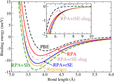
Figure 4: (Color online) Binding energy curves for Ar₂ computed with PBE and RPA-based approaches (standard RPA, RPA+SE, RPA+rSE, and RPA+rSE-diag based on PBE), in comparison with the Tang-Toennies reference curve. The results are obtained using the Gaussian “aug-cc-pV6Z” T. H. Dunning (1989) basis set. The basis set superposition error (BSSE) is corrected here and in all following calculations using the counterpoise correction scheme.Boys and Bernardi (1970)

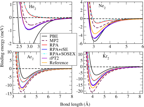
Figure 5: (Color online) Binding energy curves for rare-gas dimers computed with RPA-based approaches, in comparison with PBE, MP2, and the Tang-Toennies reference curves. He₂, Ne₂, and Ar₂ results are obtained using the aug-cc-pV6Z basis set, and Kr₂ using the aug-cc-pV5Z basis set. All RPA-type calculations are based on the PBE reference.

The full set of binding energy curves for He₂, Ne₂, Ar₂, and Kr₂ obtained with PBE, MP2, RPA, rPT2, as well as the “intermediate” schemes RPA+rSE and RPA+SOSEX are then shown in Fig. 5. PBE does not contain long-range dispersion interactions by construction, and therefore decays too fast at large separations. Around the equilibrium region, PBE vastly overbinds He₂ and Ne₂, and underbinds Ar₂ and Kr₂. MP2 shows the opposite trend, although it performs better at a quantitative level. RPA systematically underbinds all dimers. This underbinding is most significant for He₂ and Ne₂. Adding the rSE correction leads to a substantial improvement for all dimers. With the largest available Dunning Gaussian basis sets T. H. Dunning (1989) (aug-cc-pV6Z for He, Ne, Ar and aug-cc-pV5Z for Kr), RPA+rSE shows nearly perfect agreement with the reference curve for He₂, overshoots a little bit for Ne₂, and slightly underbinds Ar₂ and Kr₂. The SOSEX correction, on the other hand, has very little effect on the binding energies of these purely dispersion-bonded systems. As a result, rPT2 lies almost on top of RPA+rSE. The overall accuracy of RPA+rSE and rPT2 for rare-gas dimers is very satisfactory, in particular since no adjustable parameters are used in these schemes.

III.1.2 S22 and S66 test sets

A widely used benchmark set for weak interactions are the S22 molecular complexes designed by Jurečka et al., Jurečka et al. (2006) for which accurate reference interaction energies obtained using the the CCSD(T) method are available. Takatani et al. (2010) This molecular test set includes the most common types of non-covalent interactions: hydrogen bonding, dispersion-dominated bonding, and those of mixed character. The performance of RPA and some of the RPA-related methods have been benchmarked for this test set. Zhu et al. (2010); Eshuis and Furche (2011); Ren et al. (2011); Eshuis and Furche (2012) Similar to correlated quantum chemical methods, the quality of basis sets for RPA calculations is a significant issue.Furche (2001); Eshuis and Furche (2012); Fabiano and Dalla Sala (2012) Using our numerical atomic orbital (NAO) tier 4 basis plus additional diffuse Gaussian functions from the aug-cc-pV5Z set (denoted as “tier 4 + a5Z-d”Ren et al. (2012b); see also Appendix D), we obtained a mean absolute error (MAE) of 0.90 kcal/mol in RPA@PBE for S22, fairly close to the 0.79 kcal/mol reported by Eshuis and Furche Eshuis and Furche (2012) using Dunning’s Gaussian basis sets extrapolated to the complete basis set (CBS) limit. In Appendix D the convergence behavior of these two types of basis sets is shown for the methane dimer. In this work we will continue to use the “tier 4 + a5Z-d” basis set, bearing in mind that the absolute numbers could carry an uncertainty of 0.1 kcal/mol (4 meV), which will however not affect our discussion here.

In Fig. 6 the relative errors from RPA+rSE, RPA+SOSEX, and rPT2 are presented for each individual molecule of the S22 set. Results from RPA and RPA+SE, as well as from PBE and MP2 are also included for comparison. PBE and MP2 are both performing well for hydrogen-bonded molecules where the electrostatic interactions dominate, but PBE underbinds the dispersion-dominated and those of mixed-character significantly, while the opposite is true for MP2. RPA-based methods are performing much better than PBE and MP2 for these two types of interactions. RPA+rSE falls between RPA and RPA+SE, although it lies closer to RPA+SE. For hydrogen-bonded molecules, RPA+rSE improves over RPA+SE, with the latter overbinding these molecules noticeably. Moreover, it is interesting to note that RPA+SOSEX improves over RPA appreciably for hydrogen- and mixed-bonding, but much less so for dispersion-bonded molecules. This is consistent with its performance for rare-gas dimers. Now, combining rSE and SOSEX, rPT2 performs equally well or better for dispersion-dominated and mixed-bonding, but overshoots significantly for hydrogen-bonding. So far this is the only case we have found, for which combining rSE and SOSEX worsens the description. Finally we note that for $\pi$-stacked systems like the benzene dimer (# 11) RPA gives a substantial error, but neither rSE nor SOSEX significantly improves upon RPA. This warrants further attention in future studies.

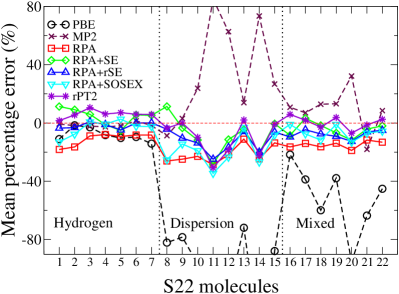
Figure 6: (Color online) The percentage errors for the S22 test set for RPA-derived computational schemes (based on PBE reference orbitals), in comparison to PBE and MP2. The CCSD(T)/CBS results of Takatani et al. Takatani et al. (2010) are used as reference. Lines are guides to the eye.

Recently the S22 test set has been extended to an even larger, more comprehensive and balanced test set called S66.Řezáč et al. (2011) This overcomes several shortcomings of S22, e.g. the strong bias towards nucleic-acid-like structures. We also performed benchmark calculations with RPA, rPT2, and related computational schemes for this test set, and the results are presented in Fig. 7. The overall performance for S66 is very similar to that observed for S22. In brief, RPA+rSE performs better (or slightly better) than RPA+SE, which itself is a significant improvement over the standard RPA method. Adding SOSEX, the resultant rPT2 approach performs even (slightly) better than RPA+rSE for dispersion and mixed interactions. However, this is not the case for hydrogen bonds, where rPT2 clearly overshoots and the strength of hydrogen bonds becomes overestimated. Overall, for weak interactions RPA+rSE outperforms other computational schemes benchmarked here, and yields a MAE of 10.1 meV (or 0.23 kcal/mol).

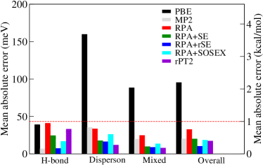
Figure 7: (Color online) MAEs (in both meV and kcal/mol) for the S66 test set given by RPA, rPT2 and related schemes (based on PBE reference orbitals), in addition to PBE and MP2. The CCSD(T) results of Rezac et al. Řezáč et al. (2011) at the CBS limit are used here as reference.

III.2 G2 atomization energies

The atomization energy of molecules is a key quantity in thermochemistry. RPA has been tested for this quantity in early works,Furche (2001); Paier et al. (2010) where a pronounced underbinding behavior was observed. In a recent work, Paier et al. Paier et al. (2012) reported a detailed study of the atomization energies of the G2-I setCurtiss et al. (1997) using RPA and its variants, including the rPT2-diag scheme as discussed before. To test the influence of the off-diagonal elements of rSE in the rPT2 scheme, we present in Fig. 8 the MAEs for RPA, rPT2-diag, rPT2, and related methods. Some of these results were already included in our recent review paper on RPA.Ren et al. (2012a) In brief, the MAE for RPA is significantly reduced when adding the (r)SE or SOSEX corrections. In this case, RPA+rSE yields a slightly larger MAE than RPA+SE. Combining the rSE and SOSEX corrections, rPT2 reduces the MAE further by a factor of two. In contrast to the nonbonded interactions discussed in the previous section, the difference between rPT2 and rPT2-diag is small (0.18 kcal/mol or 8 meV difference in MAE). validating our previous conclusions regarding the atomization energies in Ref. Paier et al., 2012 that were based on the rPT2-diag scheme.

In this context we would like to warn that, despite the success of RPA+SOSEX and rPT2 for describing the atomization energies on average, adding SOSEX to RPA makes things worse (more underbinding) for certain molecules (in particular O₂ and N₂), and this problem also carries over to rPT2. A detailed investigation of this issue is beyond the scope of this paper, and will be carried out in future work.

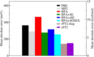
Figure 8: The MAEs (in both meV and kcal/mol) of the G2-I atomization energies Curtiss et al. (1997) obtained with PBE, MP2, RPA, rPT2, and related methods. The Gaussian cc-pV6Z basis set T. H. Dunning (1989) was used in all calculations. Reference data are from Ref. Feller and Peterson, 1998.

III.3 Barrier heights

To complete our discussion, we address chemical reaction barrier heights. For this purpose we chose the HTBH38 and NHTBH38 test set of Truhlar and coworkers. Zhao et al. (2005); Zhao and Truhlar (2006) RPA-based methods were benchmarked in previous studiesPaier et al. (2012); Eshuis et al. (2012); Ren et al. (2012a), and we here revisit this set with the upgraded version of rPT2. The MAEs for our different schemes are shown in Fig. 9. Standard RPA performs remarkably well for reaction barrier heights compared to all alternatives. This has been rationalized by Henderson and Scuseria Henderson and Scuseria (2010) to be due to the inherent self-correlation error in RPA that mimics “static correlation” (i.e. the (near) degeneracy of two (or more) determinants), leading to an excellent description of the transition states due to partial error cancellation. Unfortunately, any attempt to correct RPA deteriorates its performance in this case. In particular, the RPA+SE method provides a bad description of the transition states, resulting in errors that are even larger than in PBE. The RPA+SE error reduces when the SE term is renormalized in RPA+rSE. The errors in RPA+rSE and RPA+SOSEX tend to cancel each other, and by combining the two schemes, rPT2 gives a much more satisfactory description of the barrier heights. Similar to the G2-I test set, the difference between rPT2 and rPT2-diag is small (0.33 kcal/mol for HTBH38 and 0.25 kcal/mol for NHTBH38 in MAE) compared to the variation among other schemes.

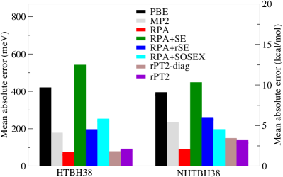
Figure 9: (Color online) The MAEs (in both meV and kcal/mol) of the HTBH38 and NHTBH38 test sets for barrier heights, obtained with PBE, MP2, RPA, rPT2, and related methods (based on PBE). Reference data are from Ref. Zhao et al., 2005; Zhao and Truhlar, 2006. Gaussian cc-pV6Z basis sets were used in all calculations.

IV Conclusions

In summary, the rPT2 method comprises an infinite summation of three distinct series of diagrams: RPA, SOSEX, and rSE. As is obvious from its diagrammatic representation, rPT2 can be viewed as a renormalization of bare second-order perturbation theory – the latter being the leading term of rPT2. In this work we derived an alternative way to express the SOSEX correlation energy, discussed in detail how to sum up the “off-diagonal” elements in rSE, which were neglected in previous works, and presented the concept of rPT2 from a diagrammatic point of view. We benchmarked the performance of rPT2 and related approaches (RPA+rSE, RPA+SOSEX), focusing on weakly interacting molecules. We found that rPT2 works well for dispersion and mixed-type interactions, but for hydrogen bonds it over-corrects the underbinding behavior of RPA. We also examined the influence of the previously neglected “off-diagonal” elements in the rSE correction and found that, for weak interactions, it is crucial to include them, whereas for atomization energy and reaction barrier heights, the off-diagonal elements only have a minor effect. We also found that the SOSEX correction improves the description of electrostatic interactions substantially, but has very little effect on dispersion interactions. rSE, on the other hand, leads to a better description of both electrostatic and dispersion interactions.

Overall rPT2 provides a conceptually appealing, and diagrammatically systematic way for going beyond RPA. Although it does not always deliver the best accuracy in every single case compared to other RPA-based approaches, it provides the most “balanced” description across various different electronic and chemical environments. We thus consider the rPT2 scheme as a natural step for extending and improving the RPA method. The successes and shortcomings of rPT2 documented in this work provide a useful basis for developing more accurate, robust, and generally applicable electronic structure methods in the coming years.

Appendix A Implementation of AC-SOSEX in FHI-aims

The RPA implementation in FHI-aims has been described in detail in Ref. Ren et al., 2012b. Here we will give a brief account of the SOSEX implementation in our code. The energy expression that we would like to evaluate is

$$E_{c}^{\text{AC-SOSEX}}=-\frac{1}{2\pi}\int_{0}^{\infty}d\omega \sum_{ia,jb}\langle ij|ba\rangle\langle ij|\bar{W}(i\omega)|ab\rangle\times$$

$${\cal F}_{ia}(i\omega){\cal F}_{jb}(i\omega)\,$$ (27)

where $\langle ij|ba\rangle$ are the two-electron Coulomb integrals defined in Eq. (5), and $\langle ij|\bar{W}(i\omega)|ab\rangle$ are the corresponding (coupling-constant-averaged) screened Coulomb integrals. The frequency-dependent factor ${\cal F}_{ia}(i\omega)$ is defined in Eq. (18).

In analogy to the RPA case, the basic technique to evaluate the two-electron integrals in our code is the resolution-of-identity. We chose the Coulomb metric, denoted “RI-V” in the following. Here we would like to emphasize that “RI-V” is a highly accurate method, and the error incurred thereby is vanishingly small for practical purposes (see Ref. Ren et al., 2012b for detail benchmarks). In RI-V, the bare two-electron integrals are computed as

$$\langle ij|ab\rangle=\sum_{\mu\nu}(ia|\mu)V_{\mu\nu}^{-1}(\nu|ib)\,\\$$ (28)

where

$$(ia|\mu)=\iint d{\bf r}d{\bf r^{\prime}}\frac{\psi_{i}({\bf r})\psi_{a}({\bf r})P_{\mu}({\bf r^{\prime}})}{|{\bf r}-{\bf r^{\prime}}|}\,,$$ (29)

and

$$V_{\mu\nu}=\iint d{\bf r}d{\bf r^{\prime}}\frac{P_{\mu}({\bf r})P_{\nu}({\bf r^{\prime}})}{|{\bf r}-{\bf r^{\prime}}|}\,.$$ (30)

Here $\psi_{p}$ are canonical single-particle spin-orbitals, and $P_{\mu}({\bf r})$ are a set of suitably constructed auxiliary basis functions.Ren et al. (2012b) For notational simplicity all orbitals are assumed to be real.

In practice, we decompose the $V^{-1}$ matrix in Eq. (28) into the product of its square roots, and combine each three-index integral with a square root. This gives

$$\langle ij|ab\rangle=\sum_{\mu}O_{ia}^{\mu}O_{jb}^{\mu}\,\\$$ (31)

with

$$O_{ia}^{\mu}=\sum_{\nu}(ia|\nu)V^{-1/2}_{\nu\mu}\,.$$ (32)

As discussed in the context of the $GW$ implementation in FHI-aims, Ren et al. (2012b) the “RI-V” technique can be used to treat the screened two-electron Coulomb integrals as well. In this case we have

$$\langle ij|\bar{W}(i\omega)|ab\rangle=\sum_{\mu,\nu}O_{ia}^{\mu}\bar{\cal E}^{-1}_{\mu\nu}(i\omega)O_{jb}^{\mu}$$ (33)

where $\bar{\cal E}$ is the coupling-constant averaged dielectric functions, formally linked to the screened Coulomb matrix by

$$\bar{\cal E}^{-1}(i\omega)=V^{-1/2}\bar{W}(i\omega)V^{-1/2}\,.$$ (34)

In Eq. (34), $\bar{W}(i\omega)$ is the screened Coulomb interaction matrix represented in terms of the auxiliary basis set,

$$\bar{W}_{\mu\nu}(i\omega)=\iint d{\bf r}d{\bf r^{\prime}}P_{\mu}({\bf r})\bar{W}_{\mu\nu}({\bf r},{\bf r^{\prime}},i\omega)P_{\nu}({\bf r^{\prime}}).$$ (35)

For convenience, we introduce a quantity $\Pi(i\omega)=v^{1/2}\chi_{0}(i\omega)v^{1/2}$, where $\chi_{0}(i\omega)$ is the independent density response function defined in Eq. (2). Using Eqs. (2), (29), and (32), one can easily obtain the matrix representation of $\Pi(i\omega)$ in the auxiliary basis

$$\Pi_{\mu\nu}(i\omega)=\sum_{ia}\frac{2(\epsilon_{i}-\epsilon_{a})}{\omega^{2}+(\epsilon_{i}-\epsilon_{a})^{2}}O_{ia}^{\mu}O_{ia}^{\nu}\,$$ (36)

where $\epsilon_{i}$ and $\epsilon_{a}$ are occupied and unoccupied single-particle orbital energies, respectively. Using Eq. (14), the matrix form of $\bar{\cal E}^{-1}$ becomes

$$\bar{\cal E}^{-1}(i\omega)=\int_{0}^{1}d\lambda\left[1-\lambda\Pi(i\omega)\right]^{-1}\lambda\,.$$ (37)

The $\lambda$-integration in Eq. (37) can be accurately computed using a Gauss-Legendre quadrature with 5-6 grid points.

Combining Eqs (27), (31), and (33), the final expression for the RI-SOSEX energy is

$$E_{\text{c}}^{\text{SOSEX}} = -\frac{1}{2\pi}\int_{0}^{\infty}d\omega\sum_{ij,ab}\left[\left(\sum_{\mu}O_{ia}^{\mu}O_{jb}^{\mu}\right)\left(\sum_{\nu\gamma}O_{ia}^{\nu}\bar{\cal E}_{\nu\gamma}^{-1}(i\omega)O_{jb}^{\gamma}\right)\right]{\cal F}_{ia}(i\omega){\cal F}_{jb}(i\omega)\,.$$ (38)

The computational effort for evaluating Eq. (38) formally scales as $O(N^{5})$, where $N$ is the system size.

Appendix B Derivation of the single excitation contribution to the 2nd-order correlation energy

In this section we derive Eq. (22) that is presented in the main part of this paper – the single excitation contribution to the 2nd-order correlation energy – from Rayleigh-Schrödinger perturbation theory (RSPT). The interacting $N$-electron system at hand is governed by the Hamiltonian

$$\hat{H}=\sum_{j=1}^{N}\left[-\frac{1}{2}\nabla^{2}_{j}+\hat{v}_{\text{ext}}({\bf r}_{j})\right]+\sum_{j<k}^{N}\frac{1}{|{\bf r}_{j}-{\bf r}_{k}|},$$

where $\hat{v}_{\text{ext}}({\bf r})$ is a local, multiplicative external potential. In RSPT, $\hat{H}$ is partitioned into a non-interacting mean-field Hamiltonian $\hat{H}^{0}$ and an interacting perturbation $\hat{H}^{\prime}$,

$$\hat{H} = \hat{H}^{0}+\hat{H}^{\prime}$$

$$\hat{H}^{0} = \sum_{j=1}^{N}\hat{h}^{0}(j)=\sum_{j=1}^{N}\left[-\frac{1}{2}\nabla^{2}_{j}+\hat{v}_{\text{ext}}({\bf r}_{j})+\hat{v}^{\text{MF}}_{j}\right]$$

$$\hat{H}^{\prime} = \sum_{j<k}^{N}\frac{1}{|{\bf r}_{j}-{\bf r}_{k}|}-\sum_{j=1}^{N}\hat{v}^{\text{MF}}_{j}.$$

Here $\hat{v}^{\text{MF}}$ is any mean-field potential, which can be non-local, as in the case of Hartree-Fock (HF) theory, or local, as in the case of Kohn-Sham (KS) theory.

Suppose the solution of the single-particle Hamiltonian $\hat{h}^{0}$ is known

$$\hat{h}^{0}|\psi_{p}\rangle=\epsilon_{p}|\psi_{p}\rangle,$$ (39)

then the solution of the non-interacting many-body Hamiltonian $H^{0}$ follows directly

$$\hat{H}^{0}|\Phi_{n}\rangle=E^{(0)}_{n}|\Phi_{n}\rangle.$$

The $|\Phi_{n}\rangle$ are single Slater determinants formed from $N$ of the spin orbitals $|p\rangle=|\psi_{p}\rangle$ determined in Eq. (39). These Slater determinants can be distinguished according to their excitation level: the ground-state configuration $|\Phi_{0}\rangle$, singly excited configurations $|\Phi_{i}^{a}\rangle$, doubly excited configurations $|\Phi_{ij}^{ab}\rangle$, etc., where $i,j,k,\dots$ denotes occupied orbitals and $a,b,c,\dots$ unoccupied ones. Following standard perturbation theory, the single-excitation (SE) contribution to the 2nd-order correlation energy is given by

$$E^{\text{SE}}_{c} = \sum_{i}\sum_{a}\frac{|\langle\Phi_{0}|\hat{H}^{\prime}|\Phi_{i}^{a}\rangle|^{2}}{E^{(0)}_{0}-E^{(0)}_{ia}}$$

$$= \sum_{i}\sum_{a}\frac{|\langle\Phi_{0}|\sum_{j<k}^{N}\frac{1}{|{\bf r}_{j}-{\bf r}_{k}|}-\sum_{j=1}^{N}\hat{v}^{\text{MF}}_{j}|\Phi_{i}^{a}\rangle|^{2}}{\epsilon_{i}-\epsilon_{a}}$$

where we have used the fact $E^{(0)}_{0}-E^{(0)}_{i,a}=\epsilon_{i}-\epsilon_{a}$.

To proceed, the numerator of Eq. (LABEL:Eq:SE_expression) needs to be evaluated. This can most easily be done using second-quantization

$$\sum_{j<k}^{N}\frac{1}{|{\bf r}_{j}-{\bf r}_{k}|} \rightarrow \frac{1}{2}\sum_{pqrs}\langle pq|rs\rangle c_{p}^{\dagger}c_{q}^{\dagger}c_{s}c_{r},$$

$$\sum_{i=j}^{N}\hat{v}^{\text{MF}}_{j} \rightarrow \sum_{pq}\langle p|\hat{v}^{\text{MF}}|q\rangle c_{p}^{\dagger}c_{q},$$

where $p,q,r,s$ are arbitrary spin-orbitals from Eq. (39), $c_{p}^{\dagger}$ and $c_{q}$, etc. are the electron creation and annihilation operators, and $\langle pq|rs\rangle$ the two-electron Coulomb integrals

$$\langle pq|rs\rangle=\int d{\bf r}d{\bf r^{\prime}}\frac{\psi_{p}^{\ast}({\bf r})\psi_{r}({\bf r})\psi_{q}^{\ast}({\bf r^{\prime}})\psi_{s}({\bf r^{\prime}})}{|{\bf r}-{\bf r^{\prime}}|}.$$

The expectation value of the two-particle Coulomb operator between the ground-state configuration $\Phi_{0}$ and the single excitation $\Phi_{i}^{a}$ is given by

$$\displaystyle\langle\Phi_{0}|\frac{1}{2}\sum_{pqrs}\langle pq|rs\rangle c_{p}^{\dagger}c_{q}^{\dagger}c_{s}c_{r}|\Phi_{i}^{a}\rangle = \sum_{p}^{\text{occ}}\left[\langle ip|ap\rangle-\langle ip|pa\rangle\right]$$ (41)

$$= \langle\psi_{i}|\hat{v}^{\text{HF}}|\psi_{a}\rangle$$

where $v^{\text{HF}}$ is the HF single-particle potential.

The expectation value of the mean-field single-particle operator $\hat{v}^{\text{MF}}$, on the other hand, is given by

$$\langle\Phi_{0}|\sum_{pq}\langle p|\hat{v}^{\text{MF}}|q\rangle c_{p}^{\dagger}c_{q}|\Phi_{i}^{a}\rangle=\langle\psi_{i}|\hat{v}^{\text{MF}}|\psi_{a}\rangle$$ (42)

Combining Eqs. (LABEL:Eq:SE_expression), (41), and (42), one gets

$$E_{c}^{\text{SE}} = \sum_{i}\sum_{a}\frac{|\langle\psi_{i}|\hat{v}^{\text{HF}}-\hat{v}^{\text{MF}}|\psi_{a}\rangle|^{2}}{\epsilon_{i}-\epsilon_{a}}$$ (43)

$$= \sum_{i}\sum_{a}\frac{|\Delta v_{ia}|^{2}}{\epsilon_{i}-\epsilon_{a}},$$

where $\Delta v_{ia}$ is the matrix element of the difference between the HF potential $\hat{v}^{\text{HF}}$ and the single-particle mean-field potential $\hat{v}^{\text{MF}}$ in question.

Observing that the $\psi$’s are eigenstates of $\hat{h}^{0}=-\frac{1}{2}\nabla^{2}+v_{\text{ext}}+v^{\text{MF}}$, and hence all non-diagonal elements $\langle\psi_{i}|\hat{h}^{0}|\psi_{a}\rangle$ are zero, one can alternatively express Eq. (43) as

$$E_{c}^{\text{SE}} = \sum_{i}\sum_{a}\frac{|\langle\psi_{i}|-\frac{1}{2}\nabla^{2}+\hat{v}_{\text{ext}}+\hat{v}^{\text{HF}}|\psi_{a}\rangle|^{2}}{\epsilon_{i}-\epsilon_{a}}$$ (44)

$$= \sum_{i}\sum_{a}\frac{|\langle\psi_{i}|\hat{f}|\psi_{a}\rangle|^{2}}{\epsilon_{i}-\epsilon_{a}}$$

where $\hat{f}$ is the single-particle HF Hamiltonian, or simply Fock operator. Thus Eq. (22) in the main paper is derived.

For the HF reference state, i.e., when $\hat{v}^{\text{MF}}=\hat{v}^{\text{HF}}$, the $\psi$’s are eigenstates of the Fock operator, and hence Eq. (LABEL:Eq:SE_expression) is zero. For any other reference state, e.g., a KS reference state, the $\psi$’s are no longer eigenstates of the Fock operator, and Eq. (LABEL:Eq:SE_expression) is in general not zero. This gives rise to a finite SE contribution to the second-order correlation energy.

Appendix C Derivation of the renormalized single excitation (rSE) contribution

We start with the expression for the second-order single-excitation (SE) contribution discussed in Appendix B

$$E_{\text{c}}^{\text{SE}}=\sum_{i,a}\frac{\langle\Phi_{0}|\hat{H^{\prime}}|\Phi_{i}^{a}\rangle\langle\Phi_{i}^{a}|\hat{H^{\prime}}|\Psi_{0}\rangle}{E^{(0)}_{0}-E^{(0)}_{ia}}\,.$$ (45)

The form of this equation actually already implies that the singly excited states $|\Phi_{i}^{a}\rangle$ are Slater determinants composed of canonical orbitals, namely $|\Psi_{i}^{a}\rangle=\text{Det}\left\{\psi_{q}\right\}$ where $\hat{h}^{0}|\psi_{q}\rangle=\epsilon_{q}|\psi_{q}\rangle$, and $\hat{H}_{0}|\Phi_{i}^{a}\rangle=E^{(0)}_{ia}|\Phi_{i}^{a}\rangle$ with $E^{(0)}_{ia}=E^{(0)}_{0}+\epsilon_{a}-\epsilon_{i}$. Appendix B shows that Eq. (45) can be reduced to the simple expression in Eq (44) that is given in terms of (canonical) single-particle orbitals.

To set the stage for later discussions, we can also more generally express the SE energy in Eq. (45) in terms of non-canonical orbitals $\{\chi_{q}\}$, where $\hat{h}^{0}|\chi_{p}\rangle=\sum_{q}h^{0}_{pq}|\chi_{q}\rangle$, and $h^{0}_{pq}=\langle\chi_{p}|\hat{h}^{0}|\chi_{q}\rangle$. In this case, $E_{\text{c}}^{\text{SE}}$ is given by

$$E_{\text{c}}^{\text{SE}} =\sum_{ij,ab}\langle\Phi_{0}|\hat{H^{\prime}}|\Phi_{i}^{a}\rangle\langle\Phi_{i}^{a}|(E^{(0)}_{0}-\hat{H}_{0})^{-1}|\Phi_{j}^{b}\rangle\langle\Phi_{j}^{b}|\hat{H^{\prime}}|\Phi_{0}\rangle$$

$$=\sum_{ij,ab}\langle\chi_{i}|\hat{f}|\chi_{a}\rangle\left[(E^{(0)}_{0}I-H_{0})^{-1}\right]_{ia,jb}\langle\chi_{b}|\hat{f}|\chi_{j}\rangle\,,$$ (46)

where $I$ is the identity matrix: $I_{ia,jb}=\delta_{ij}\delta_{ab}$, and

$$\left[E^{(0)}_{0}I-H_{0}\right]_{ia,jb} =\langle\Phi_{i}^{a}|E^{(0)}_{0}-\hat{H}_{0}|\Phi_{j}^{b}\rangle$$

$$=h^{0}_{ij}\delta_{ab}-h^{0}_{ab}\delta_{ij}\,.$$ (47)

Now the question arises how to sum up all the higher-order SE diagrams shown in Fig. 2? For canonical orbitals, the corresponding algebraic expression can be easily obtained by applying the rules of evaluating Goldstone diagrams.Szabo and Ostlund (1989)

$$E_{\text{c}}^{\text{rSE}}= \sum_{ia}\frac{f_{ai}f_{ia}}{\epsilon_{i}-\epsilon_{a}}-\sum_{ij,a}\frac{f_{ai}\Delta v_{ij}f_{ja}}{(\epsilon_{i}-\epsilon_{a})(\epsilon_{j}-\epsilon_{a})}+\sum_{i,ab}\frac{f_{ai}f_{ib}\Delta v_{ba}}{(\epsilon_{i}-\epsilon_{a})(\epsilon_{i}-\epsilon_{b})}$$

$$+ \sum_{ijk,a}\frac{f_{ai}\Delta v_{ik}\Delta v_{kj}f_{ja}}{(\epsilon_{i}-\epsilon_{a})(\epsilon_{k}-\epsilon_{a})(\epsilon_{j}-\epsilon_{a})}+\sum_{i,abc}\frac{f_{ai}f_{ib}\Delta v_{bc}\Delta v_{ca}}{(\epsilon_{i}-\epsilon_{a})(\epsilon_{i}-\epsilon_{b})(\epsilon_{i}-\epsilon_{c})}$$

$$- \sum_{ij,ab}\frac{f_{ai}\Delta v_{ij}f_{jb}\Delta v_{ba}}{(\epsilon_{i}-\epsilon_{a})(\epsilon_{j}-\epsilon_{a})(\epsilon_{j}-\epsilon_{b})}-\sum_{ij,ab}\frac{f_{ai}\Delta v_{ij}f_{jb}\Delta v_{ba}}{(\epsilon_{i}-\epsilon_{a})(\epsilon_{i}-\epsilon_{b})(\epsilon_{j}-\epsilon_{b})}$$ (48)

$$+ \cdots$$

where $\Delta v_{pq}=\langle\psi_{p}|\hat{f}-\hat{h}_{0}|\psi_{q}\rangle$, and $\Delta v_{ia}=f_{ia}=\langle\psi_{i}|\hat{f}|\psi_{a}\rangle$. To see how the infinite-order summation in Eq (C) is carried out, we rearrange the expression as follows:

$$E_{\text{c}}^{\text{rSE}}= \sum_{ij,ab}\frac{f_{ai}\delta_{ij}\delta_{ab}f_{jb}}{\epsilon_{i}-\epsilon_{a}}+\sum_{ij,ab}\frac{f_{ai}\left(\Delta v_{ab}\delta_{ij}-\Delta v_{ij}\delta_{ab}\right)f_{jb}}{(\epsilon_{i}-\epsilon_{a})(\epsilon_{j}-\epsilon_{b})}+$$

$$\sum_{ijk,abc}\frac{f_{ai}\left(\Delta v_{ik}\Delta v_{kj}\delta_{ac}\delta_{bc}+\Delta v_{bc}\Delta v_{ca}\delta_{ik}\delta_{kj}-\Delta v_{ik}\Delta v_{bc}\delta_{jk}\delta_{ac}-\Delta v_{kj}\Delta v_{ca}\delta_{ik}\delta_{bc}\right)f_{jb}}{(\epsilon_{i}-\epsilon_{a})(\epsilon_{k}-\epsilon_{c})(\epsilon_{j}-\epsilon_{b})}+\cdots$$

$$= \sum_{ij,ab}\frac{f_{ai}}{\epsilon_{i}-\epsilon_{a}}\left[\delta_{ij}\delta_{ab}+\Omega_{ia,jb}+(\Omega^{2})_{ia,jb}+\cdots\right]f_{jb}$$

$$= \sum_{ij,ab}\frac{f_{ai}}{\epsilon_{i}-\epsilon_{a}}\left[(I-\Omega)^{-1}\right]_{ia,jb}f_{jb}$$ (49)

where we have introduced the $\Omega$ matrix, defined as

$$\Omega_{ia,jb}=\frac{\Delta v_{ba}\delta_{ij}-\Delta v_{ij}\delta_{ab}}{\epsilon_{j}-\epsilon_{b}}\,.$$ (50)

Further denoting $A_{ia,jb}=(\epsilon_{i}-\epsilon_{a})\delta_{ij}\delta_{ab}$, one observes

$$\frac{1}{\epsilon_{i}-\epsilon_{a}}\left[(I-\Omega)^{-1}\right]_{ia,jb} =\left[A^{-1}((I-\Omega)^{-1}\right]_{ia,jb}$$

$$=\left[(A-\Omega A)^{-1}\right]_{ia,jb}\,,$$ (51)

and

$$(A-\Omega A)_{ia,jb} =(\epsilon_{i}-\epsilon_{a})\delta_{ij}\delta_{ab}+\Delta v_{ij}\delta_{ab}-\Delta v_{ba}\delta_{ij}$$

$$=f_{ij}\delta_{ab}-f_{ab}\delta_{ij}\,,$$ (52)

where $f_{ij}=\epsilon_{i}\delta_{ij}+\Delta v_{ij}$, $f_{ab}=\epsilon_{a}\delta_{ab}+\Delta v_{ab}$ have been used. It follows that

$$E_{\text{c}}^{\text{rSE}}=\sum_{ij,ab}f_{ai}\left[(A-\Omega A)^{-1}\right]_{ia,jb}f_{jb}\,.$$ (53)

We observe that the rSE energy expressed in terms of canonical orbitals via Eqs. (52) and (53) has the same mathematical structure as the second-order SE energy expressed in terms of non-canonical orbitals given by Eq. (46) and (47). The difference is that now the corresponding matrix elements in the denominator are evaluated using the Fock operator $\hat{f}$, instead of the KS Hamiltonian operator $\hat{h}^{0}$.

To simplify the evaluation of Eq. (53), one can rotate the occupied orbitals and unoccupied orbitals separately, such that the Fock matrix becomes diagonal in the occupied and unoccupied subspaces. This procedure is called semi-canonicalization. To be more precise, suppose there are transformation matrices ${\cal O}$ and ${\cal U}$ which diagonalize the $f_{ij}$ and $f_{ab}$ blocks separately

$$\sum_{k}f_{ik}{\cal O}_{kj}={\cal O}_{ij}\tilde{\epsilon}_{j}$$

$$\sum_{c}f_{ac}{\cal U}_{cb}={\cal U}_{ab}\tilde{\epsilon}_{b}\,.$$ (54)

We then have

$$\sum_{kl,cd}{\cal O}^{\ast}_{ik}{\cal U}^{\ast}_{ac}(A-\Omega A)_{kc,ld}{\cal O}_{lj}{\cal U}_{db}=\delta_{ij}\delta_{ab}(\tilde{\epsilon}_{j}-\tilde{\epsilon}_{b})\,$$ (55)

or equivalently,

$$\left[(A-\Omega A)^{-1}\right]_{ia,jb}=\sum_{k,c}{\cal O}_{ik}{\cal U}_{ac}(\tilde{\epsilon}_{k}-\tilde{\epsilon}_{c})^{-1}{\cal O}_{kj}^{\ast}{\cal U}_{cb}^{\ast}\,.$$ (56)

Inserting Eq. (56) into Eq. (53), one arrives at

$$E_{\text{c}}^{\text{rSE}}=\sum_{ia}\frac{\tilde{f}_{ai}\tilde{f}_{ia}}{\tilde{\epsilon}_{i}-\tilde{\epsilon}_{a}}\,.$$ (57)

where

$$\tilde{f}_{ia}=\sum_{jb}{\cal O^{\ast}}_{ij}{\cal U^{\ast}}_{ab}f_{jb}\,.$$ (58)

Thus the final expression for rSE has the same form as that for SE, only the eigenvalues $\epsilon_{i},\epsilon_{a}$ and the “transition amplitude” $f_{ia}$ have to be reinterpreted. The actual implementation following Eqs. (54), (57), and (58) is straightforward.

Appendix D Basis convergence

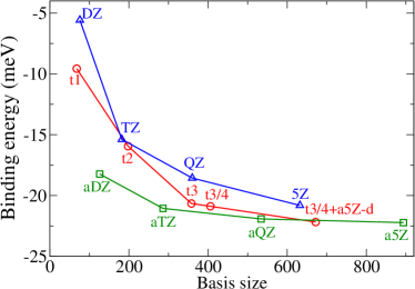
Figure 10: (Color online) The rPT2@PBE binding energy of methane dimer in its equilibrium geometry as a function of the basis set size. “XZ” and “aXZ” (X=D,T,Q,5) denote respectively the Dunning “cc-pVXZ” and “aug-cc-pVXZ” basis, whereas “tN” denotes the FHI-aims “tier N” basis, and “t3/4” here means tier 4 basis for C and tier 3 basis for H (note that a tier 4 basis for H is not available). “t3/4+a5Z-d” corresponds to the NAO “tier 3/4” plus diffuse functions from aug-cc-pV5Z. The BSSE is corrected.

Figure 4 shows the convergence behavior of the rPT2 binding energy of the methane dimer (in its equilibrium geometry) with respect to the FHI-aims NAO “tier N” basis as well as Dunning’s “cc-pVXZ” and “aug-cc-pVXZ” basis. The methane dimer is dominated by the dispersion interaction, and the so-called “diffuse functions” are needed to accurately describe this interaction. The difference between the “cc-pVXZ” and “aug-cc-pVXZ” results highlight the importance of including “diffuse functions”. For methane dimer the “tier N” series exhibits a faster convergence than “cc-pVXZ” whereas a slower convergence than “aug-cc-pVXZ” for BSSE-corrected binding energies. When adding diffuse functions from aug-cc-pV5Z to “tier 3/4”, (called “t3/4+a5Z-d” in Fig. 10) results of similar quality as the full aug-cc-pV5Z basis are obtained.

References

- Hohenberg and Kohn (1964) P. Hohenberg and W. Kohn, Phys. Rev. 136, B864 (1964).
- Kohn and Sham (1965) W. Kohn and L. J. Sham, Phys. Rev. 140, A1133 (1965).
- Perdew and Schmidt (2001) J. P. Perdew and K. Schmidt, in Density Functional Theory and its Application to Materials , edited by V. Van Doren, C. Van Alsenoy, and P. Geerlings (AIP, Melville, NY, 2001).
- Bohm and Pines (1953) D. Bohm and D. Pines, Phys. Rev. 92, 609 (1953).
- Gell-Mann and Brueckner (1957) M. Gell-Mann and K. A. Brueckner, Phys. Rev. 106, 364 (1957).
- Langreth and Perdew (1977) D. C. Langreth and J. P. Perdew, Phys. Rev. B 15, 2884 (1977).
- Gunnarsson and Lundqvist (1976) O. Gunnarsson and B. I. Lundqvist, Phys. Rev. B 13, 4274 (1976).
- Eshuis et al. (2012) H. Eshuis, J. E. Bates, and F. Furche, Theor. Chem. Acc. p. 1 (2012).
- Ren et al. (2012a) X. Ren, P. Rinke, C. Joas, and M. Scheffler, J. Mater. Sci. 47, 7447 (2012a).
- Furche (2001) F. Furche, Phys. Rev. B 64, 195120 (2001).
- Feibelman et al. (2001) P. J. Feibelman, B. Hammer, J. K. Nørskov, F. Wagner, M. Scheffler, R. Stumpf, R. Watwe, and J. Dumestic, J. Phys. Chem. B 105, 4018 (2001).
- Ren et al. (2009) X. Ren, P. Rinke, and M. Scheffler, Phys. Rev. B 80, 045402 (2009).
- Schimka et al. (2010) L. Schimka, J. Harl, A. Stroppa, A. Grüneis, M. Marsman, F. Mittendorfer, and G. Kresse, Nature Materials 9, 741 (2010).
- Casadei et al. (2012) M. Casadei, X. Ren, P. Rinke, A. Rubio, and M. Scheffler, Phys. Rev. Lett. 109, 146402 (2012).
- Harl and Kresse (2008) J. Harl and G. Kresse, Phys. Rev. B 77, 045136 (2008).
- Harl and Kresse (2009) J. Harl and G. Kresse, Phys. Rev. Lett. 103, 056401 (2009).
- Janesko et al. (2009a) B. G. Janesko, T. M. Henderson, and G. E. Scuseria, J. Chem. Phys. 130, 081105 (2009a).
- Janesko et al. (2009b) B. G. Janesko, T. M. Henderson, and G. E. Scuseria, J. Chem. Phys. 131, 154115 (2009b).
- Toulouse et al. (2009) J. Toulouse, I. C. Gerber, G. Jansen, A. Savin, and J. G. Ángyán, Phys. Rev. Lett. 102, 096404 (2009).
- Ren et al. (2011) X. Ren, A. Tkatchenko, P. Rinke, and M. Scheffler, Phys. Rev. Lett. 106, 153003 (2011).
- Lu et al. (2009) D. Lu, Y. Li, D. Rocca, and G. Galli, Phys. Rev. Lett. 102, 206411 (2009).
- Eshuis and Furche (2011) H. Eshuis and F. Furche, J. Phys. Chem. Lett. 2, 983 (2011).
- Paier et al. (2010) J. Paier, B. G. Janesko, T. M. Henderson, G. E. Scuseria, A. Grüneis, and G. Kresse, J. Chem. Phys. 132, 094103 (2010), erratum: ibid. 133, 179902 (2010).
- Caruso et al. (2012) F. Caruso, D. R. Rohr, M. Hellgren, X. Ren, P. Rinke, A. Rubio, and M. Scheffler, Phys. Rev. Lett. submitted (2012), arXiv:1210.8300.
- Yan et al. (2000) Z. Yan, J. P. Perdew, and S. Kurth, Phys. Rev. B 61, 16430 (2000).
- Grüneis et al. (2009) A. Grüneis, M. Marsman, J. Harl, L. Schimka, and G. Kresse, J. Chem. Phys. 131, 154115 (2009).
- Heßelmann (2011) A. Heßelmann, J. Chem. Phys. 134, 204107 (2011).
- Heßelmann and Görling (2011) A. Heßelmann and A. Görling, Phys. Rev. Lett. 106, 093001 (2011).
- Ruzsinszky et al. (2011) A. Ruzsinszky, J. P. Perdew, and G. I. Csonka, J. Chem. Phys. 134, 114110 (2011).
- Ángyán et al. (2011) J. G. Ángyán, R.-F. Liu, J. Toulouse, and G. Jansen, J. Chem. Theory Comput. 7, 3116 (2011).
- Olsen and Thygesen (2012) T. Olsen and K. S. Thygesen, Phys. Rev. B 86, 081103(R) (2012).
- Freeman (1977) D. L. Freeman, Phys. Rev. B 15, 5512 (1977).
- Goldstone (1957) J. Goldstone, Proc. Roy. Soc. (London) A239, 267 (1957).
- Paier et al. (2012) J. Paier, X. Ren, P. Rinke, G. E. Scuseria, A. Grüneis, G. Kresse, and M. Scheffler, New J. Phys. 14, 043002 (2012).
- Jurečka et al. (2006) P. Jurečka, J. Šponer, J. Černý, and P. Hobza, Phys. Chem. Chem. Phys. 8, 1985 (2006).
- Řezáč et al. (2008) J. Řezáč, P. Jurečka, K. E. Riley, J. Černý, H. Valdes, K. Pluháčková, K. Berka, T. Řezáč, M. Pitoňák, J. Vondrášek, et al., Collect. Czech. Chem. Commun. 73, 1261 (2008).
- Řezáč et al. (2011) J. Řezáč, K. E. Riley, and P. Hobza, J. Chem. Theo. Comp 7, 2427 (2011).
- Curtiss et al. (1997) L. A. Curtiss, K. Raghavachari, P. C. Redfern, and J. A. Pople, J. Chem. Phys. 106, 1063 (1997).
- Zhao et al. (2005) Y. Zhao, N. González-García, and D. G. Truhlar, J. Phys. Chem. A 109, 2012 (2005).
- Zhao and Truhlar (2006) Y. Zhao and D. G. Truhlar, J. Chem. Phys. 125, 194101 (2006).
- Jansen et al. (2010) G. Jansen, R.-F. Liu, and J. G. Ángyán, J. Chem. Phys. 133, 154106 (2010).
- Blum et al. (2009) V. Blum, F. Hanke, R. Gehrke, P. Havu, V. Havu, X. Ren, K. Reuter, and M. Scheffler, Comp. Phys. Comm. 180, 2175 (2009).
- Ren et al. (2012b) X. Ren, P. Rinke, V. Blum, J. Wieferink, A. Tkatchenko, A. Sanfilippo, K. Reuter, and M. Scheffler, New J. Phys. 14, 053020 (2012b).
- Furche (2008) F. Furche, J. Chem. Phys. 129, 114105 (2008).
- Scuseria et al. (2008) G. E. Scuseria, T. M. Henderson, and D. C. Sorensen, J. Chem. Phys. 129, 231101 (2008).
- Henderson and Scuseria (2010) T. M. Henderson and G. E. Scuseria, Mol. Phys. 108, 2511 (2010).
- Dunlap et al. (1979) B. I. Dunlap, J. W. D. Connolly, and J. R. Sabin, J. Chem. Phys 71, 3396 (1979).
- Feyereisen et al. (1993) M. Feyereisen, G. Fitzgerald, and A. Komornicki, Chem. Phys. Lett. 208, 359 (1993).
- Weigend et al. (1998) F. Weigend, M. Häser, H. Patzelt, and R. Ahlrichs, Chem. Phys. Lett. 294, 143 (1998).
- (50) Gaussian Development Version, Revision G.01, M. J. Frisch et. al., Gaussian, Inc., Wallingford CT, 2007.
- Perdew et al. (1996) J. P. Perdew, K. Burke, and M. Ernzerhof, Phys. Rev. Lett 77, 3865 (1996).
- Görling and Levy (1993) A. Görling and M. Levy, Phys. Rev. B 47, 13105 (1993).
- Bartlett (2010) R. J. Bartlett, Mol. Phys. 108, 3299 (2010).
- Jiang and Engel (2006) H. Jiang and E. Engel, J. Chem. Phys. 125, 184108 (2006).
- Schweigert et al. (2006) I. V. Schweigert, V. F. Lotrich, and R. J. Bartlett, J. Chem. Phys. 125, 104108 (2006).
- Fetter and Walecka (1971) A. L. Fetter and J. D. Walecka, Quantum Theory of Many-Particle Systems (McGraw-Hill, New York, 1971).
- Grüneis et al. (2010) A. Grüneis, M. Marsman, and G. Kresse, J. Chem. Phys. 133, 074107 (2010).
- (58) X. Ren et al., unpublished.
- Harl et al. (2010) J. Harl, L. Schimka, and G. Kresse, Phys. Rev. B 81, 115126 (2010).
- Curtiss et al. (2005) L. A. Curtiss, P. C. Redfern, and K. Raghavachari, J. Chem. Phys. 123, 124107 (2005).
- Szabo and Ostlund (1977) A. Szabo and N. S. Ostlund, J. Chem. Phys. 67, 4351 (1977).
- Dobson (1994) J. F. Dobson, in Topics in Condensed Matter Physics, edited by M. P. Das (Nova, New York, 1994).
- Dobson and Gould (2012) J. F. Dobson and T. Gould, J. Phys.: Condens. Matter 24 (2012).
- Lu et al. (2010) D. Lu, H.-V. Nguyen, and G. Galli, J. Chem. Phys. 133, 154110 (2010).
- Furche and Van Voorhis (2005) F. Furche and T. Van Voorhis, J. Chem. Phys. 122, 164106 (2005).
- Li et al. (2010) Y. Li, D. Lu, H.-V. Nguyen, and G. Galli, J. Phys. Chem. A 114, 1944 (2010).
- Zhu et al. (2010) W. Zhu, J. Toulouse, A. Savin, and J. G. Ángyán, J. Chem. Phys. 132, 244108 (2010).
- Toulouse et al. (2011) J. Toulouse, W. Zhu, A. Savin, G. Jansen, and J. G. Ángyán, J. Chem. Phys. 135, 084119 (2011).
- Tang and Toennies (2003) K. T. Tang and J. P. Toennies, J. Chem. Phys. 118, 4976 (2003).
- Klopper and Noga (1995) W. Klopper and J. Noga, J. Chem. Phys. 103, 6127 (1995).
- LASCHUK et al. (2003) E. F. LASCHUK, M. M. MARTINS, and S. EVANGELISTI, Int. J. Quan. Chem. 95, 303 (2003).
- T. H. Dunning (1989) J. T. H. Dunning, J. Chem. Phys. 90, 1007 (1989).
- Boys and Bernardi (1970) S. F. Boys and F. Bernardi, Mol. Phys. 19, 553 (1970).
- Takatani et al. (2010) T. Takatani, E. G. Hohenstein, M. Malagoli, M. S. Marshall, and C. D. Sherrill, J. Chem. Phys. 132, 144104 (2010).
- Eshuis and Furche (2012) H. Eshuis and F. Furche, J. Chem. Phys. 136, 084105 (2012).
- Fabiano and Dalla Sala (2012) E. Fabiano and F. Dalla Sala, Theor. Chem. Acc. 131, 1278 (2012).
- Feller and Peterson (1998) D. Feller and K. A. Peterson, J. Chem. Phys. 108, 154 (1998).
- Szabo and Ostlund (1989) A. Szabo and N. S. Ostlund, Modern Quantum Chemistry: Introduction to Advanced Electronic Structure Theory (McGraw-Hill, New York, 1989).