Abstract

We study evolution equations for electric and magnetic field amplitudes in a ring cavity with plane mirrors. The cavity is filled with a positive or negative refraction index material with third order effective electric and magnetic non-linearities. Two coupled non-linear equations for the electric and magnetic amplitudes are obtained. We prove that the description can be reduced to one Lugiato Lefever equation with generalized coefficients. A stability analysis of the homogeneous solution, complemented with numerical integration, shows that any combination of the parameters should correspond to one of three characteristic behaviors.

PACS: 42.65.Sf, 05.45.-a

1 Introduction

During the last decade, composite material developments allowed the experimental realization of materials with negative refraction index [1, 2], theoretically predicted by Veselago [3]. These materials have simultaneously a negative dielectric permittivity and negative magnetic permeability, a property that is not found in natural materials. Negative refraction index materials (NRM) have many new and interesting properties, such as a refracted wave on the same side as the incoming wave respect to the surface normal and Poynting vector in the direction opposite to wave-vector. A number of applications has been proposed based on their new properties, such as perfect lenses, phase compensators, and electrically small antennas [4, 5, 6, 7].

Most studies on NRM consider linear relations between electric field and polarization, and magnetic field and magnetization. The study of nonlinear effects acquired an increasing interest during the last years. It is known that the propagation of an electromagnetic wave in a Kerr nonlinear material, with positive refraction index, can be described by a nonlinear order parameter equation of the Schrödinger type [8], and that the same kind of equation can be extended to an NRM [9, 10, 11, 12, 13]. Nevertheless, it has been shown [14, 15] that a composite metamaterial with negative refraction index can develop a non-linear macroscopic magnetic response. This means that, although the host medium has a negligible magnetic non-linearity, the periodic inclusions of the metamaterial produce an effective magnetic non-linear response when the wave-length is much larger than the periodicity of the inclusions. In the rest of the paper, when we speak about magnetic non-linearity we refer to this macroscopic magnetic response present only in metamaterials. Electric and magnetic non-linearities in composite materials have been also analyzed in, for example, [16, 17, 18, 19]

In this paper, we are interested in the analysis of the equations that describe the electric and magnetic fields in a ring cavity with plane mirrors containing a material with negative or positive refraction index and with electric and magnetic non-linearities. The aim of the work is to obtain a simple mathematical description of this system, useful to identify relevant parameters and to analyze typical behaviours.

The paper is organized as follows. In Sect. 2 we present the equations for the evolution of the electric and magnetic field amplitudes in a ring cavity (the derivation, starting from two coupled non-linear Schrödinger equations, is in the appendix), and show that the description can be reduced to one Lugiato Lefever equation [20] with generalized parameters. In Sect. 3, we analyze the effects of dissipation. In Sect. 4 we use a linear stability analysis to identify three typical situations that arise depending on the signs of the three parameters of the equation. Numerical integration supports and completes the previous analysis. In Sect. 5 we present our conclusions.

2 Equations in the cavity

The equations that describe the behavior of the electric and magnetic fields in a plane perpendicular to light propagation are of the type of the Lugiato-Lefever (LL) equation. The LL equation is a simple mean field model that has been useful for the analysis of pattern formation in a cavity with flat mirrors containing a Kerr medium and driven by a coherent plane-wave field, see also [21, 22].

We will first analyze the problem of free propagation (without mirrors) of an electromagnetic wave in the material and afterwards will use the resulting equations to derive the behavior in the cavity.

We will consider a linearly polarized driving field with frequency $\omega_{0}$. Let us suppose that the electric field is in the $x$ direction and the magnetic field is in the $y$ direction. The starting point are the Maxwell’s equations and the constitutive relations for the electric displacement, $D=\epsilon_{0}E+P$, and the magnetic induction, $B=\mu_{0}H+\mu_{0}M$. (There is an interesting alternative approach, described in [23], in which the fields $E$, $D$ and $B$ are used, with $D=\tilde{\varepsilon}E$ and $B=H$, where $\tilde{\varepsilon}$ is a generalized dielectric constant.)

Considering an isotropic metamaterial with third order non-linearities, the non-linear relation between polarization $P$ (in the $x$ direction) and electric field $E$ is

$$P(t)=\epsilon_{0}\int_{-\infty}^{\infty}\chi^{(1)}_{e}(t-\tau)\,E(\tau)\,d\tau+\epsilon_{0}\int_{-\infty}^{\infty}\chi^{(3)}_{e}(t-\tau_{1},t-\tau_{2},t-\tau_{3})\,E(\tau_{1})E(\tau_{2})E(\tau_{3})\,d\tau_{1}d\tau_{2}d\tau_{3},$$ (1)

where $\chi^{(1)}_{e}$ and $\chi^{(3)}_{e}$ are the linear and nonlinear electric susceptibilities [8]. The same geometric arguments used in (1) can be applied to the relation between magnetization $M$ and magnetic field $H$:

$$M(t)=\int_{-\infty}^{\infty}\chi^{(1)}_{m}(t-\tau)\,H(\tau)\,d\tau+\int_{-\infty}^{\infty}\chi^{(3)}_{m}(t-\tau_{1},t-\tau_{2},t-\tau_{3})\,H(\tau_{1})H(\tau_{2})H(\tau_{3})\,d\tau_{1}d\tau_{2}d\tau_{3},$$ (2)

with $\chi^{(1)}_{m}$ and $\chi^{(3)}_{m}$ being the linear and nonlinear magnetic susceptibilities. Let us remark that $\chi^{(1)}_{e}$, $\chi^{(3)}_{e}$, $\chi^{(1)}_{m}$ and $\chi^{(3)}_{m}$ describe macroscopic effective response of the metamaterial valid for a driving field with a wave-length much larger than the periodicity of the inclusions. We are assuming that the field intensities are small enough in order to neglect higher order terms. The effective macroscopic magnetic non-linearity can become relevant in metamaterials, as shown in [14], in contrast with what happens in conventional optics, where magnetic non-linearities are negligible.

The classical multiple-scales perturbation technique will be applied, in which it is assumed that the light is quasimonochromatic and can be represented by a plane wave, with frequency $\omega_{0}$ and wave-number $k_{0}$, propagating along the $z$ axis and modulated by a slowly varying envelope. The envelope depends on space $\mathbf{R}=(X,Y,Z)$ and time $T$ variables that have characteristic scales much greater than the scales given by $1/k_{0}$ and $1/\omega_{0}$. The fields $E$ and $H$ can be written in the following way

$$E = \mathcal{E}(\mathbf{R},T)e^{i(k_{0}z-\omega_{0}t)}+c.c.$$

$$H = \mathcal{H}(\mathbf{R},T)e^{i(k_{0}z-\omega_{0}t)}+c.c.$$ (3)

where $\mathcal{E}$ and $\mathcal{H}$ are the slowly varying amplitudes. Similar relations hold for $P$ and $M$.

Let us define the wave-number $k(\omega)=\omega n(\omega)/c$; the refraction index is $n(\omega)=\pm\sqrt{\epsilon_{r}(\omega)\,\mu_{r}(\omega)}$ (it takes the negative sign when both, $\epsilon_{r}$ and $\mu_{r}$ are negative [3]), where $\epsilon_{r}(\omega)=1+\chi^{(1)}_{e}(\omega)$ and $\mu_{r}(\omega)=1+\chi^{(1)}_{m}(\omega)$ are the relative permittivity and the relative permeability respectively. In particular, $k_{0}=\omega_{0}n/c$, with $n=n(\omega_{0})$, and we call $k^{\prime}$ and $k^{\prime\prime}$ the derivatives of $k(\omega)$ evaluated in $\omega=\omega_{0}$.

The details of the application of the multiple-scales technique in our case are essentially the same to the ones described in Ref. [8], Sect. 2k, for a positive refraction index material with only electric non-linearity. After this process, we arrive to the following coupled non linear Schrödinger equations for the envelopes of the electric and magnetic fields:

$$\frac{\partial\mathcal{E}}{\partial\xi} = -\frac{ik^{\prime\prime}}{2}\frac{\partial^{2}\mathcal{E}}{\partial t^{2}}+\frac{i}{2k_{0}}\nabla_{\perp}^{2}\mathcal{E}+\frac{i3k_{0}}{2}\left(\frac{\chi^{(3)}_{e}}{\epsilon_{r}}|\mathcal{E}|^{2}+\frac{\chi^{(3)}_{m}}{\mu_{r}}|\mathcal{H}|^{2}\right)\mathcal{E}$$ (4)

$$\frac{\partial\mathcal{H}}{\partial\xi} = -\frac{ik^{\prime\prime}}{2}\frac{\partial^{2}\mathcal{H}}{\partial t^{2}}+\frac{i}{2k_{0}}\nabla_{\perp}^{2}\mathcal{H}+\frac{i3k_{0}}{2}\left(\frac{\chi^{(3)}_{e}}{\epsilon_{r}}|\mathcal{E}|^{2}+\frac{\chi^{(3)}_{m}}{\mu_{r}}|\mathcal{H}|^{2}\right)\mathcal{H}$$ (5)

where, in the left hand side, the transformation $\xi=z$, $\tau=t-k^{\prime}z$, was used; the transverse Laplacian $\nabla_{\perp}=(\frac{\partial^{2}}{\partial x^{2}},\frac{\partial^{2}}{\partial y^{2}})$ is defined in the plane perpendicular to the $z$ axis. The relative permittivity and the relative permeability, $\epsilon_{r}$ and $\mu_{r}$, are evaluated in $\omega_{0}$. The non-linear electric and magnetic susceptibilities, $\chi^{(3)}_{e}$ and $\chi^{(3)}_{m}$, are the Fourier transforms evaluated in $(\omega_{0},\omega_{0},-\omega_{0})$. Dissipation (linear or non-linear) is neglected, so that $\chi^{(1)}_{e}$, $\chi^{(1)}_{m}$, $\chi^{(3)}_{e}$ and $\chi^{(3)}_{m}$ are real quantities. This is an often met approximation in conventional optics, but dissipation could play a relevant role in metamaterials. In this section we will derive the equations for a material without dissipation, and in Sect. 3 we will analyze how these equations are modified when dissipation is taken into account.

The nonlinear electric susceptibility is usually written as $\chi^{(3)}_{e}=\alpha/E_{c}^{2}$, where $\alpha=\pm 1$ stands for a focusing or defocusing nonlinearity and $E_{c}$ is a characteristic electric field. Eqs. (4) and (5) are an extension of the analysis performed in [9, 10] to include the magnetic non-linearity, and are similar to the ones derived in [13].

For an NRM, $k_{0}$ is negative, but this does not modify the sign of the non-linear terms in Eqs. (4) and (5), since $k_{0}/\epsilon_{r}$ and $k_{0}/\mu_{r}$ are always positive. The difference appears in the diffraction term, that becomes negative for an NRM.

Figure 1: Ring cavity with the nonlinear optic material of size $L$.

Fig. 1 shows the geometry of the ring cavity. At the entrance mirror, the input field has amplitudes $E_{\mathrm{in}}$ and $H_{\mathrm{in}}$, with $H_{\mathrm{in}}=E_{\mathrm{in}}\sqrt{\epsilon_{0}/\mu_{0}}$. The non-linear material has length $L$, the transmission coefficient in the right end of the material for the electric field amplitude is $t_{+}=1+\zeta$, and for the magnetic field amplitude is $t_{-}=1-\zeta$, where $\zeta=(\eta-\eta_{0})/(\eta+\eta_{0})$ with $\eta_{0}=\sqrt{\epsilon_{0}/\mu_{0}}$ and $\eta=\sqrt{\epsilon/\mu}$. The transmission and reflection coefficients in the input mirror are $t_{i}$ and $r_{i}$. The time of a round trip is $T_{r}$, the phase accumulated by the wave in a round trip is $\phi$, and the detuning between the pump field and the cavity mode is $\theta=\phi\;\mathrm{mod}\;2\pi$, with $\theta\ll 1$ since we consider that the cavity is close to resonance. It is convenient to define the quantity $\rho=|r_{i}|(1-\zeta^{2})$, the length $l=\sqrt{L\rho/[2|k_{0}|(1-\rho)]}$, and the characteristic electric field $C=t_{+}E_{c}\sqrt{2\epsilon_{r}(1-\rho)/(3Lk_{0}\rho)}$. Using the non-linear Schrödinger equations (4) and (5) for the fields inside the cavity, and after the following change of variables:

$$A_{1}=\frac{\mathcal{E}}{C},\quad A_{2}=\frac{\mathcal{H}}{C}\sqrt{\frac{\mu_{0}}{\epsilon_{0}}},\quad x^{\prime}=x/l, y^{\prime}=y/l,\quad t^{\prime}=t\frac{(1-\rho)}{T_{r}},$$ (6)

we arrive to two Lugiato-Lefever type equations (the details of the derivation can be found in the appendix):

$$\frac{\partial A_{1}}{\partial t}=A_{\mathrm{in}}-(1+i\Theta)A_{1}+i\beta\nabla^{2}_{\perp}A_{1}+i(\alpha|A_{1}|^{2}+\gamma|A_{2}|^{2})A_{1}$$ (7)

$$\frac{\partial A_{2}}{\partial t}=A_{\mathrm{in}}-(1+i\Theta)A_{2}+i\beta\nabla^{2}_{\perp}A_{2}+i(\alpha|A_{1}|^{2}+\gamma|A_{2}|^{2})A_{2}$$ (8)

where $\Theta=-\theta\rho/(1-\rho)$, $\beta=\pm 1$ is the sign of the refraction index $n$, $\gamma=\frac{\epsilon_{0}\epsilon_{r}^{2}}{\mu_{0}\mu_{r}^{2}}\chi_{m}^{(3)}/|\chi_{e}^{(3)}|$, and $A_{\mathrm{in}}=\frac{t_{i}}{(1-\rho)}E_{\mathrm{in}}/C$. The primes have been omitted to simplify the notation.

Let us analyze the difference of the fields: $R=A_{1}-A_{2}$. It is possible to prove that $R$ decays exponentially to zero. The equation for $R$ is

$$\frac{\partial R}{\partial t}=-(1+i\Theta)R+i\beta\nabla^{2}_{\perp}R+i(\alpha|A_{1}|^{2}+\gamma|A_{2}|^{2})R,$$ (9)

from which we get

$$\frac{\partial|R|^{2}}{\partial t}=-2|R|^{2}+i\beta\bar{R}\nabla^{2}_{\perp}R-i\beta R\nabla^{2}_{\perp}\bar{R},$$ (10)

where $\bar{R}$ is the complex conjugate of $R$. We use the expression of $R$ in terms of its Fourier transform, $R(x,y,t)=\frac{1}{(2\pi)^{2}}\int dk_{x}\,dk_{y}R_{k_{x},k_{y}}e^{i(k_{x}x+k_{y}y)}$. The last two terms in Eq. (10) become

$$\bar{R}\nabla^{2}_{\perp}R-R\nabla^{2}_{\perp}\bar{R}=$$ (11)

$$\frac{1}{(2\pi)^{4}}\int dk_{x}\,dk_{y}\,dq_{x}\,dq_{y}\,R_{k_{x},k_{y}}\bar{R}_{q_{x},q_{y}}e^{i(k_{x}-q_{x})x}\,e^{i(k_{y}-q_{y})y}(q_{x}^{2}+q_{y}^{2}-k_{x}^{2}-k_{y}^{2}).$$

Let us consider the transverse average of Eq. (11), defined as the integral over the plane $x$-$y$,

$$\langle\bar{R}\nabla^{2}_{\perp}R-R\nabla^{2}_{\perp}\bar{R}\rangle=$$ (12)

$$\frac{1}{(2\pi)^{4}}\int dk_{x}\,dk_{y}\,dq_{x}\,dq_{y}\,R_{k_{x},k_{y}}\bar{R}_{q_{x},q_{y}}(q_{x}^{2}+q_{y}^{2}-k_{x}^{2}-k_{y}^{2})\int dx\,dy\,e^{i(k_{x}-q_{x})x}\,e^{i(k_{y}-q_{y})y}$$

$$= \frac{1}{(2\pi)^{2}}\int dk_{x}\,dk_{y}\,dq_{x}\,dq_{y}\,R_{k_{x},k_{y}}\bar{R}_{q_{x},q_{y}}(q_{x}^{2}+q_{y}^{2}-k_{x}^{2}-k_{y}^{2})\,\delta(k_{x}-q_{x})\,\delta(k_{y}-q_{y})$$

$$= 0.$$

Therefore, from Eq. (10) we get

$$\frac{\partial\langle|R|^{2}\rangle}{\partial t}=-2\langle|R|^{2}\rangle,$$ (13)

that means that the transverse average $\langle|R|^{2}\rangle$ decays to zero exponentially with a characteristic time 1/2 (or $T_{r}/[2(1-\rho)]$ for the previous time scale). If, after a transient, we have $\langle|R|^{2}\rangle=0$, then, since $|R|^{2}\geq 0$ in every point of the transverse plane, we have that $R=0$ in every point. Then, after a time of order 1/2, we have that $A_{1}=A_{2}$. In this situation, the description of Eqs. (7) and (8) is further simplified to

$$\frac{\partial A}{\partial t}=A_{\mathrm{in}}-(1+i\Theta)A+i\beta\nabla^{2}_{\perp}A+i\gamma^{\prime}|A|^{2}A,$$ (14)

where $A=A_{1}=A_{2}$ and $\gamma^{\prime}=\alpha+\gamma$. Eq. (14) has the same form than the Lugiato Lefever equation, but there are some differences. In the original version, that considers only an electric non-linearity, it was shown [20] that the sign of the detuning $\Theta$ must be equal to the sign of the non-linear coefficient, $\gamma^{\prime}$, but this is not necessarily the case in Eq. (14). In addition, in (14) the sign of the diffraction term, $\beta$, can be negative or positive depending on the material being an NRM or not, and the magnetic non-linearity is included in the coefficient $\gamma^{\prime}$.

In the particular case in which there is only an electric non-linearity, i.e. $\gamma=0$, and using the result of [20] that says that the sign of $\Theta$ is equal to $\alpha$, that is equal to 1 ($-1$) for a focusing (defocusing) electric non-linearity, we get,

$$\frac{\partial A}{\partial t}=A_{\mathrm{in}}-(1+i\alpha|\Theta|)A+i\beta\nabla^{2}_{\perp}A+i\alpha|A|^{2}A.$$ (15)

Eq. (15) presents an interesting symmetry. Taking its complex conjugate, and assuming that $A_{\mathrm{in}}$ is real, it can be seen that a focusing non-linearity and a positive refraction index material ($\alpha=1$ and $\beta=1$) is equivalent to the defocusing and NRM case ($\alpha=-1$ and $\beta=-1$). Also the case $(\alpha=1,\beta=-1)$ is equivalent to $(\alpha=-1,\beta=1)$. As we will see below, the equivalences are more involved when the magnetic non-linearity is considered, since the signs of the three coefficients ($\Theta$, $\beta$ and $\gamma^{\prime}$) are in general not related among them.

3 Dissipation

Although it is common to neglect dissipation in conventional optics, this is not in general an appropriate approximation for a metamaterial. In this section we analyze how the previous equations are modified when dissipation is taken into account. In this case, the electric permittivity and magnetic permeability are complex quantities. The wave-number that was defined as $k(\omega)=\frac{\omega}{c}\sqrt{\epsilon_{r}(\omega)\mu_{r}(\omega)}$ will also have an imaginary part. At the frequency $\omega_{0}$ we have

$$k(\omega_{0})=k_{0}+i\,k_{I}$$ (16)

where $k_{0}$ is the wave-number of the plane wave modulated by the slowly varying amplitude (3), and $k_{I}$ is the imaginary part.

We will consider that the attenuation distance is much larger than the wave-length. This means that $k_{I}\ll k_{0}$. In the Gigahertz range, it is possible to build an NRM with small (and even negligible) imaginary parts of $\epsilon_{r}$ and $\mu_{r}$ as was shown in, for example, [24, 25].

It is assumed that $k_{I}$ is of second order in the small parameter used in the multiple-scales perturbation technique, see [8, p. 101]. The result is an additional term in the non-linear Schrödinger equations for the envelopes of the electric and magnetic fields

$$\frac{\partial\mathcal{E}}{\partial\xi} = -\frac{ik^{\prime\prime}}{2}\frac{\partial^{2}\mathcal{E}}{\partial t^{2}}+\frac{i}{2k_{0}}\nabla_{\perp}^{2}\mathcal{E}+\frac{i3k_{0}}{2}\left(\frac{{\chi^{(3)}_{e}}}{\epsilon_{r}}|\mathcal{E}|^{2}+\frac{{\chi^{(3)}_{m}}}{\mu_{r}}|\mathcal{H}|^{2}\right)\mathcal{E}-k_{I}\mathcal{E}$$ (17)

$$\frac{\partial\mathcal{H}}{\partial\xi} = -\frac{ik^{\prime\prime}}{2}\frac{\partial^{2}\mathcal{H}}{\partial t^{2}}+\frac{i}{2k_{0}}\nabla_{\perp}^{2}\mathcal{H}+\frac{i3k_{0}}{2}\left(\frac{{\chi^{(3)}_{e}}}{\epsilon_{r}}|\mathcal{E}|^{2}+\frac{{\chi^{(3)}_{m}}}{\mu_{r}}|\mathcal{H}|^{2}\right)\mathcal{H}-k_{I}\mathcal{H}.$$ (18)

The additional terms ($-k_{I}\mathcal{E}$ and $-k_{I}\mathcal{H}$) represent an exponential decay of the amplitudes due to dissipation. In Eqs. (17) and (18), the non-linear coefficients $\chi^{(3)}_{e}/\epsilon_{r}$ and $\chi^{(3)}_{m}/\mu_{r}$ can be taken as real quantities since the contribution of the imaginary parts correspond to terms of higher order in the expansion of the small parameter.

Following the steps indicated in the appendix, we arrive to a couple of Lugiato-Lefever equations that have the same form that Eqs. (7) and (8), where now the change of variables is given by

$$A_{1}=\frac{\mathcal{E}}{C^{\prime}},\quad A_{2}=\frac{\mathcal{H}}{C^{\prime}}\sqrt{\frac{\mu_{0}}{\epsilon_{0}}},\quad x^{\prime}=x/l^{\prime}, y^{\prime}=y/l^{\prime},\quad t^{\prime}=t\frac{(1-\rho+\rho Lk_{I})}{T_{r}},$$ (19)

with $C^{\prime}=t_{+}E_{c}\sqrt{2\epsilon_{r}(1-\rho+\rho Lk_{I})/(3Lk_{0}\rho)}$ and $l^{\prime}=\sqrt{L\rho/[2|k_{0}|(1-\rho+\rho Lk_{I})]}$. The scaled detuning is now defined as $\Theta=-\theta\rho/(1-\rho+\rho Lk_{I})$, and the input field is $A_{\mathrm{in}}=\frac{t_{i}}{(1-\rho+\rho Lk_{I})}E_{\mathrm{in}}/C$. The definitions of the rest of the coefficients that appear in Eqs. (7) and (8) remain the same.

Therefore, the case of small dissipation can still be correctly described by Eqs. (7) and (8). It is not difficult to see that the demonstration of the previous section that the amplitudes $A_{1}$ and $A_{2}$ are equal after a transient still holds for this dissipative case. Consequently, the simplified description of Eq. (14) also holds.

The situation is different if the attenuation distance is of order of the wave-length, i.e., $k_{I}\sim k_{0}$, that corresponds to a factor of merit of order one. This is generally the case for optical frequencies. Now, the assumption that light can be represented by a plane wave modulated by a slowly varying amplitude, Eq. (3), is no longer valid, because the decay of the fields due to dissipation takes place in a fast space scale, and this decay can not be described by the envelopes $\mathcal{E}$ and $\mathcal{H}$. The situation when the length of the material, $L$, is much greater than the wave-length, is not interesting since no field will be detected at the output. There are many proposals to reduce losses in metamaterials, some of them are [26, 27, 28, 29, 30, 31].

4 Stability of homogeneous stationary solutions

The homogeneous stationary solutions, $A_{0}$, of Eq. (14) are obtained by solving

$$A_{\mathrm{in}}=(1+i\Theta-i\gamma^{\prime}I_{0})A_{0},$$ (20)

where $I_{0}=|A_{0}|^{2}$. For the intensities we have

$$I_{\mathrm{in}}=(1+\Theta^{2})I_{0}-2\Theta\gamma^{\prime}I_{0}^{2}+\gamma^{\prime 2}I_{0}^{3},$$ (21)

where $I_{\mathrm{in}}=|A_{\mathrm{in}}|^{2}$ is the intensity of the input field. It is well known that Eq. (21) presents bistability for $|\Theta|>\sqrt{3}$, i.e., there is a range of values of $I_{\mathrm{in}}$ for which there are two stable solutions of $I_{0}$. Note that, since $\Theta=-\theta\rho/(1-\rho)$, and $\theta\ll 1$, bistability can only be attained when $\rho=|r_{i}|(1-\zeta^{2})\simeq 1$, i.e., when the entrance mirror has a high reflectivity and the material has a high transmissivity. Another condition to have bistability is $\Theta\gamma^{\prime}>0$, this condition is automatically fulfilled when there is only an electric non-linearity, i.e., when $\gamma=0$ and $\Theta=\alpha|\Theta|$.

In terms of the solutions for the intensity $I_{0}$ obtained from (21), the homogeneous solution is

$$A_{0}=(1-i\Theta+i\gamma^{\prime}I_{0})\,I_{0}/A_{\mathrm{in}},$$ (22)

where we have assumed, without loss of generality, that $A_{\mathrm{in}}$ is real.

A linear stability analysis of $A_{0}$ gives the following eigenvalues,

$$\lambda_{\pm}=-1\pm\sqrt{[3\gamma^{\prime}I_{0}-\beta k^{2}-\Theta][\beta k^{2}+\Theta-\gamma^{\prime}I_{0}]},$$ (23)

where $k$ is the wave-number of a small perturbation. From (23) we can draw the marginal stability curves of Fig. 2. The same figure applies to both cases: negative and positive refraction index, that correspond to the negative and positive parts, respectively, of the horizontal axis. In the regions enclosed by the curves, the homogeneous solution $A_{0}$ becomes unstable. Both regions do not appear simultaneously: one corresponds to $\gamma^{\prime}>0$ and the other to $\gamma^{\prime}<0$. A value of $\Theta=0$ was used in the figure, but a different value of $\Theta$ only represents a horizontal shift of the curves. The homogeneous solution becomes unstable when the intensity is increased from zero an reaches the value $I_{0}\,|\gamma^{\prime}|=1$. Over the instability threshold, and close to it, it is known that a hexagonal pattern appears [32, 33], when the critical wave number is different from 0 (this happens when there is not bistability or, more strictly, when $\beta\Theta<2$).

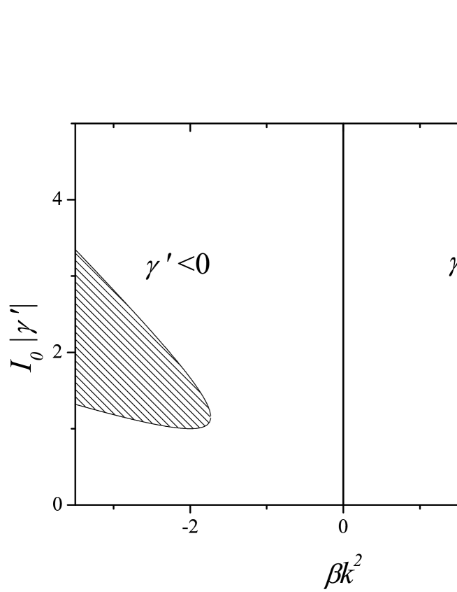
Figure 2: Marginal stability curves, $I_{0}\,|\gamma^{\prime}|$ versus $\beta k^{2}$, for $\Theta=0$. In the dashed region the homogeneous solution becomes unstable.

Eq. (14) and its complex conjugate represent the same physical situation. The only difference present in the complex conjugate equation is the sign in front of the three real parameters $\Theta$, $\beta$ and $\gamma^{\prime}$. Using this equivalence we can identify three typical situations: (a) $\beta\gamma^{\prime}>0$ and any value of $\Theta$; (b) $\beta\gamma^{\prime}<0$ and $\Theta\gamma^{\prime}<0$; and (c) $\beta\gamma^{\prime}<0$ and $\Theta\gamma^{\prime}>0$.

In case (a) $\beta$ and $\gamma^{\prime}$ have the same sign. We can see in Fig. 2 that, for $\beta=-1$ or 1, the marginal stability curve is present, so that, as the input field intensity is increased, the homogeneous solution becomes always unstable. The critical values of field intensity and wave-number are given by,

$$I_{0,c}|\gamma^{\prime}|=1\ \ \mathrm{and}\ \ k_{c}^{2}=2-|\Theta| \ \mathrm{for}\ \beta\Theta<2$$

$$I_{0,c}|\gamma^{\prime}|=2|\Theta|/3-\sqrt{\Theta^{2}-3}/3\ \ \mathrm{and}\ \ k_{c}=0 \ \mathrm{for}\ \beta\Theta>2$$

In case (b), the homogeneous solution is always stable. Bistability is not possible in this case since $\Theta\gamma^{\prime}<0$.

In case (c), the homogeneous solution becomes unstable only if there is bistability, i.e., when $|\Theta|>\sqrt{3}$. The critical values are,

$$I_{0,c}|\gamma^{\prime}|=2|\Theta|/3-\sqrt{\Theta^{2}-3}/3\ \ \mathrm{and}\ \ k_{c}=0 \ \mathrm{for}\ \sqrt{3}<|\Theta|<2$$

$$I_{0,c}|\gamma^{\prime}|=1\ \ \mathrm{and}\ \ k_{c}^{2}=|\Theta|-2 \ \mathrm{for}\ |\Theta|>2$$

If $\Theta>\sqrt{3}$, and $\gamma^{\prime}>0$, the vertical axis in Fig. 2 is shifted to the right and crosses the marginal stability curve in two points that give a range of values of $I_{0}$ for which the solution $A_{0}$ becomes unstable under homogeneous perturbations. This corresponds to the unstable branch when bistability is present. Fig. 3 shows a sequence of plots with the marginal stability curve with the values of the homogeneous solutions indicated on the vertical axis for increasing values of the input intensity $I_{\mathrm{in}}$ and for $\Theta=3$ and $\gamma^{\prime}=1$. As $I_{\mathrm{in}}$ increases from 2.9 to 2.95 a saddle node bifurcation takes place in the upper branch of the marginal stability curve (the bifurcation happens in the two dimensional phase space composed by the real and imaginary parts of $A_{0}$). As $I_{\mathrm{in}}$ is further increased, the value of the intensity of the homogeneous solution of the unstable branch (the one that is inside the instability region delimited by the curve) decreases, until it merges, in another saddle node bifurcation, with the lower homogeneous solution.

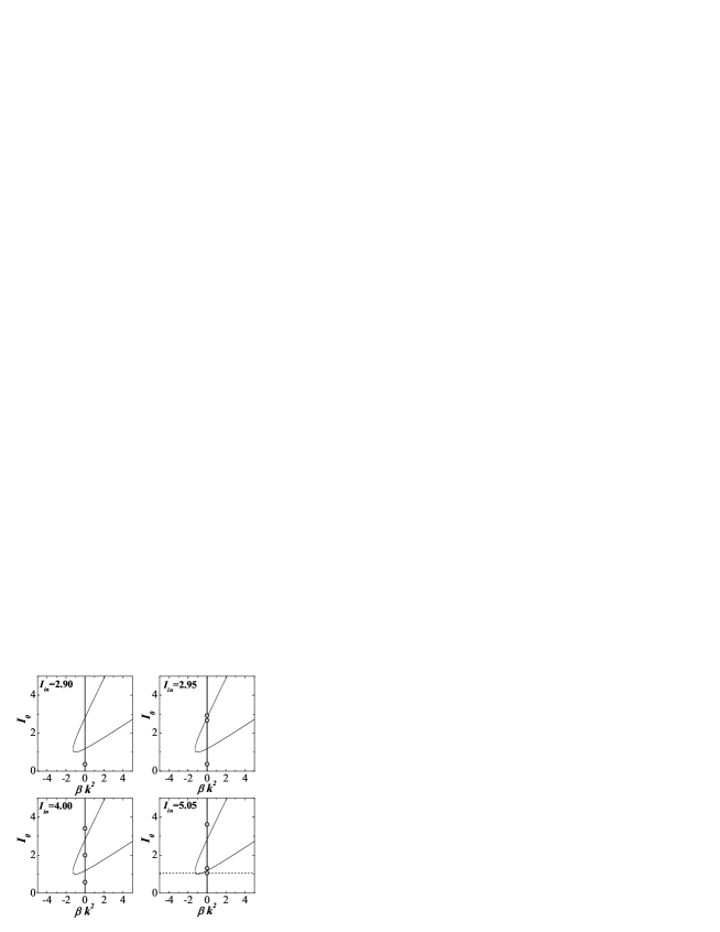
Figure 3: Marginal stability curve, $I_{0}$ versus $\beta k^{2}$, for the bistability case with $\Theta=3$, and $\gamma^{\prime}=1$. The sequence corresponds to increasing values of $I_{\mathrm{in}}$, from left to right and from top to bottom: $I_{\mathrm{in}}=2.9$, 2.95, 4 and 5.05. The small circles on the vertical axis show the positions of the homogeneous solutions. The negative horizontal axis corresponds to case (c) and the positive one to case (a).

We have an example of case (c) in Fig. 3 for $\beta=-1$, where the lower homogeneous solution becomes unstable before it merges with the homogeneous solution of the unstable branch (see dotted line in bottom right plot of Fig. 3). The saddle node bifurcation in the lower branch takes place at $I_{0}$ approximately equal to 1.18 for the parameters of Fig. 3, but a modulational instability with a wave-number different from zero takes place at a lower value of $I_{0}$ ($I_{0}=1$).

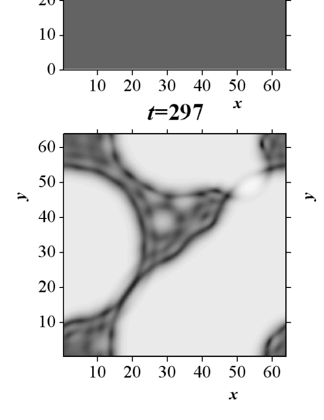
Figure 4: Four configurations of $|A|^{2}$ against position in the transverse plane, obtained from integration of Eq. (14) for increasing values of time. Parameters are $\beta=-1$, $\Theta=3$ and $\gamma^{\prime}=1$, corresponding to case (c). The initial condition has intensity $I_{0}=1.03$ ($I_{\mathrm{in}}=5.02$), slightly above the critical value ($I_{0,c}=1$). The system evolves from the lower to the upper homogeneous solution. The space and time integration steps are $\Delta x=0.25$ and $\Delta t=0.003$. The grey scale is logarithmic, black corresponds to 0.4 and white to 4.5.

Fig. 4 shows four snapshots of numerical integration results for this case. The initial condition is the lower homogeneous solution slightly above the instability threshold ($A_{0}=0.457-i0.908$, i.e. $I_{0}=1.03$), plus noise of amplitude 0.005. Eq. (14) was integrated in a square domain of 256$\times$256 points with periodic boundary conditions, using a Fourier series representation and a 4th order Runge-Kutta temporal scheme for the non-linear terms. At time $t=180$ the field still appears homogeneous. At $t=270$ a pattern characterized by the critical wave number appears ($k_{c}=1$). At $t=297$ we can see some spatial domains where the field takes the value of the upper homogeneous solution. These domains grow until the whole system becomes homogeneous. Therefore, the numerical results indicate that, as the input intensity is increased, the lower homogeneous solution becomes unstable, but this instability does not give rise to a stable non-homogeneous pattern. Instead, the system evolves to the upper homogeneous solution, that is always stable for $\beta=-1$.

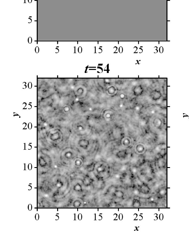
Figure 5: Intensity $|A|^{2}$ for increasing values of time calculated from Eq. (14). Parameters are $\beta=1$, $\Theta=3$ and $\gamma^{\prime}=1$, corresponding to case (a). The homogeneous initial condition has intensity equal to 1.19 plus noise of amplitude 0.005, and the input field has $I_{\mathrm{in}}=5.11$. The final state corresponds to spatiotemporal chaos that is reached independently of the value of the initial homogeneous state. Space and time integration steps: $\Delta x=0.125$ and $\Delta t=0.001$. The gray scale is logarithmic with black equal to 0.1 and white equal to 60. We used a different scale for $t=22$: black=3, white=4, in order to show the transient emerging pattern.

Continuing with the analysis of Fig. 3, the situation is different for $\beta=1$, that corresponds to case (a); in this case the lower homogeneous solution is always stable until the saddle node bifurcation takes place. Therefore, as the input intensity is increased, the lower homogeneous solution does not simply cross the marginal stability curve and lose its stability, but, instead, it does no longer exist as a stationary solution since the homogeneous mode, $k=0$, becomes unstable. We performed numerical integration of Eq. (14) for an input intensity slightly above the value corresponding to the saddle node bifurcation. For different values of the homogeneous initial condition, the evolution is qualitatively similar to the one shown in Fig. 5. Initially, only the modes close to 0 are unstable, so that, for short times, the value of the intensity increases keeping, approximately, the homogeneous shape of the field. For larger times, the system evolves to a state of optical turbulence or spatiotemporal chaos.

As mentioned before, in case (a) without bistability, an hexagonal pattern appears close and above the instability threshold. It was shown in Ref. [34] that, as the input intensity is increased, there is a sequence of different spatiotemporal regimes: oscillating hexagons, quasiperiodicity, temporal chaos and optical turbulence. When there is bistability, the state of optical turbulence is reached directly as a transition from the homogeneous state as the input intensity is increased (see Fig. 5).

The differences between the stability of homogeneous solutions for positive ($\beta=1$) or negative ($\beta=-1$) refraction index materials, when bistability is present, is clearly presented in Fig. 6. The figure shows the curve $I_{0}$ against $I_{\mathrm{in}}$. The shape of the curve is the same for $\beta=1$ or $\beta=-1$, but the stability ranges are different.

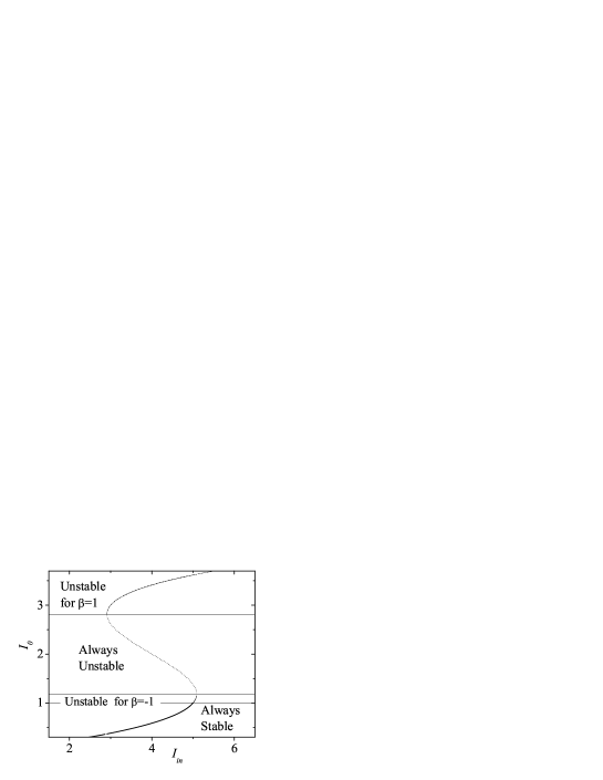
Figure 6: Intensity of the homogeneous solution $I_{0}$ against intensity of the input field $I_{\mathrm{in}}$ in the bistability case, with $\Theta=3$ and $\gamma^{\prime}=1$. The continuous curve corresponds to an always stable homogeneous solution. In the rest of the curve, the stability range depends on the sign of the refraction index, $\beta$. The part with negative slope (dotted curve) is always unstable for $\beta=1$ or $-1$. The upper part (dash-dotted curve) is unstable only for $\beta=1$ but it is stable for an NRM ($\beta=-1$). Equivalently, for the region $1<I_{0}<1.18$ the homogeneous solution is unstable for $\beta=-1$ but is stable for $\beta=1$.

The stability analysis is similar to the one presented in [9], where only an electric non-linearity was considered. The inclusion of the magnetic non-linearity is explicitly represented by factor $\gamma$ in (14). In addition, a result that, to our knowledge, was not previously reported, is the equivalence between positive and negative refraction index materials when the signs of the detuning $\Theta$ and the non-linear coefficient $\gamma^{\prime}$ are changed. This symmetry is illustrated, for example, in Fig. 2, for $\Theta=0$. In this case, the behavior for $\beta=1$ and $\gamma^{\prime}>0$ is equivalent to the behavior for $\beta=-1$ and $\gamma^{\prime}<0$.

5 Conclusions

Starting from the Maxwell equations, with non-linear polarization and magnetization, it is possible to obtain, using the multiple-scales technique, two coupled non-linear Schrödinger equations for the electric and magnetic field amplitudes. From these equations we derived the evolution of the fields in a ring cavity with plane mirrors containing a material with positive or negative refraction index and with effective electric and magnetic non-linearities. We proved that the description can be reduced to only one equation that has the same form of the Lugiato Lefever equation [20] for a positive refraction index material with only electric non-linearity.

An original contribution of the paper is the generalization of the Lugiato Lefever equation to electric and magnetic non-linearities. Let us note that, as was shown in [14], effective macroscopic magnetic non-linearities can become relevant in composite materials that are used to generate a negative refraction index. The resulting equation has three real parameters: the sign of the refraction index $\beta$, the detuning $\Theta$, and the non-linear coefficient $\gamma^{\prime}$. In the original version of the Lugiato Lefever equation, the sign of the detuning is equal to the sign of the non-linear coefficient, corresponding to the self-focusing or self-defocusing cases. In the present version, both signs are independent; in addition, the diffraction coefficient can be positive or negative depending on $\beta$. This generalization of the parameters allows the equation to represent new physical situations. Despite the fact that more free parameters necessarily makes the analysis more complex, using a linear stability analysis we have shown that any combination of the parameters must correspond to one of only three typical cases. In case (b), $\beta\gamma^{\prime}<0$ and $\Theta\gamma^{\prime}<0$, the homogeneous solution is always stable. In case (c), $\beta\gamma^{\prime}<0$ and $\Theta\gamma^{\prime}>0$, the homogeneous solution can become unstable only when there is bistability, but, in this case, numerical integration shows that the final state is the homogeneous solution of the upper branch. Only in case (a), $\beta\gamma^{\prime}>0$, the destabilization of the homogeneous solution, as the input field intensity is increased, gives rise to a non-homogeneous state. In this last case, if there is not bistability it is known that, close to the instability threshold, the asymptotic state is an hexagonal pattern. If there is bistability, numerical results for $\Theta=3$ show that there is a transition from the homogeneous state to optical turbulence as the input field is increased.

In summary, the description, in the plane perpendicular to propagation, of the evolution of the electromagnetic field in a cavity with a non-linear material with positive or negative refraction index has been reduced to a Lugiato Lefever equation with three parameters: $\Theta$, $\gamma^{\prime}$ and $\beta$. These quantities are functions of the much larger set of parameters of the original description (based on the Maxwell equations). One of the aims of the work was the identification of relevant parameters since they allow a better understanding of typical behaviours that the system can develop. This kind of analysis is much more difficult to perform with the original description.

Acknowledgements

We thank Carlos Martel for helpful discussions. This work was partially supported by Consejo Nacional de Investigaciones Científicas y Técnicas (CONICET, Argentina), Agencia Nacional de Promoción Científica y Tecnológica ANPCyT (PICT 2004, N 17-20075, Argentina) and Universidad Politécnica de Madrid (Spain) under grant AL09-P(I+D).

Appendix

In this appendix we present the derivation of the cavity equations (7) and (8) starting from the non linear Schrödinger equations (4) and (5). It is essentially an extension of the procedure described in [9] to the case of electric and magnetic non-linearity.

Using Eqs. (4) and (5), for a small distance $\delta\xi$, we can write

$$\mathcal{F}_{\pm}(\xi+\delta\xi)=\mathcal{F}_{\pm}(\xi)+i\,\delta\xi\,\hat{N}\mathcal{F}_{\pm}(\xi)\simeq e^{i\,\delta\xi\,\hat{N}}\mathcal{F}_{\pm}(\xi)$$ (24)

where $\mathcal{F}_{+}=\mathcal{E}$, $\mathcal{F}_{-}=\mathcal{H}$, and $\hat{N}$ is the operator

$$\hat{N}=-\frac{k^{\prime\prime}}{2}\frac{\partial^{2}}{\partial t^{2}}+\frac{1}{2k_{0}}\nabla_{\perp}^{2}+\frac{3k_{0}}{2}\left(\frac{\chi^{(3)}_{e}}{\epsilon_{r}}|\mathcal{E}|^{2}+\frac{\chi^{(3)}_{m}}{\mu_{r}}|\mathcal{H}|^{2}\right)$$ (25)

Fig. 1 shows the scheme of the cavity with the non linear material of length $L$ whose left and right ends are at positions $a$ and $b$. We call $a_{+}$ and $a_{-}$ the positions immediately to the right and to the left of $a$ respectively, and similarly for $b_{+}$ and $b_{-}$. Using the impedance of free space, $\eta_{0}=\sqrt{\epsilon_{0}/\mu_{0}}$, and of the material, $\eta=\sqrt{\epsilon/\mu}$, the transmission coefficient for the electric field amplitude, when light goes from $b_{-}$ to $b_{+}$, is

$$t_{+}=\frac{2\eta}{\eta+\eta_{0}}=1+\zeta$$ (26)

where $\zeta=(\eta-\eta_{0})/(\eta+\eta_{0})$ is a small quantity, so that the transmission coefficient is close to 1. (Even when $\eta$ is not close to $\eta_{0}$, a transmission coefficient close to 1 can be achieved by filling the cavity with a substance with an impedance close to $\eta$.) The transmission coefficient for the magnetic field amplitude in $b$ is,

$$t_{-}=\frac{2\eta_{0}}{\eta+\eta_{0}}=1-\zeta.$$ (27)

Using also the transmission and reflection coefficients in the input mirror, $t_{i}$ and $r_{i}$, we obtain the following relations

$$\mathcal{F}_{\pm}(b_{+}) = t_{\pm}\mathcal{F}_{\pm}(b_{-})$$

$$\mathcal{F}_{\pm}(a_{+}) = t_{\mp}\mathcal{F}_{\pm}(a_{-})$$

$$\mathcal{F}_{\pm}(a_{-}) = |r_{i}|e^{i\phi}\mathcal{F}_{\pm}(b_{+})+t_{i}F_{\mathrm{in}\pm}$$ (28)

where $F_{\mathrm{in}+}=E_{\mathrm{in}}$, $F_{\mathrm{in}-}=H_{\mathrm{in}}$, and $\phi$, the phase accumulated in a round trip, includes the phase change of $4\pi$ due to reflection in the four mirrors. We will consider that the system is close to resonance so that the detuning is $\theta\ll 1$, with $\theta=\phi\ \mathrm{mod}\ 2\pi$. Let $\mathcal{F}_{*\pm}$ be the value of $\mathcal{F}_{\pm}$ after one round trip in the cavity, that takes a time $T_{r}$. Applying the relations (24) and (28) we find (subindices $\pm$ are removed for simplicity)

$$\mathcal{F}_{*}=t_{i}F_{in}+|r_{i}|(1-\zeta^{2})e^{i\theta}e^{iL\hat{N}}\mathcal{F}\simeq t_{i}F_{in}+|r_{i}|(1-\zeta^{2})(1+i\theta+iL\hat{N})\mathcal{F}.$$ (29)

According to (25), the operator $\hat{N}$ depends on the fields inside the material, but, in Eq. (29), $\mathcal{F}$ corresponds to the fields outside the material, so $\hat{N}$ should be evaluated in $t_{\mp}\mathcal{F}_{\pm}$. Writing the time derivative of $\mathcal{F}$ as $(\mathcal{F}_{*}-\mathcal{F})/T_{r}$, and defining $\rho=|r_{i}|(1-\zeta^{2})$, we obtain,

$$T_{r}\frac{\partial\mathcal{F}}{\partial t}=t_{i}F_{in}+(\rho-1)\mathcal{F}+i\rho\theta\mathcal{F}+i\rho L\,\hat{N}\mathcal{F}.$$ (30)

After replacing the operator $\hat{N}$ by its definition (25), and using the change of variables defined by Eqs. (6), we arrive to Eqs. (7) and (8) for the amplitudes of the electric and magnetic fields in the cavity. It can be shown that, in the cavity equations, the dispersion term proportional to $k^{\prime\prime}$ in (25) can be neglected.

References

- [1] D.R. Smith, W.J. Padilla, D.C. Vier, S.C. Nemat-Nasser and S. Schultz, Phys. Rev. Lett. 84 4184 (2000)
- [2] R.A. Shelby, D.R. Smith and S. Schultz, Science 292 77 (2001).
- [3] V.G. Veselago, Usp. Fiz. Nauk 92 517 (1967); V.G. Veselago, Sov. Phys.-Usp. 10 509 (1968).
- [4] Z. Jakšić, N. Dalarsson and M. Maksimović, Microwave Review 12(1), 36-49 (2006).
- [5] S.A. Ramakrishna, Rep. Prog. Phys. 68, 449 (2005).
- [6] A. Grbic and G.V. Eleftheriades, Physical Review Letters 92, 117403 (2004).
- [7] N. Fang, H. Lee, C. Sun and X. Zhang, Science 308, 534-537 (2005).
- [8] J.V. Moloney and A.C. Newell, Nonlinear Optics (Westview Press, Boulder, Colorado, 2003).
- [9] P. Kockaert, P. Tassin, G. Van der Sande, I. Veretennicoff and M. Tlidi, Phys. Rev. A 74, 033822 (2006); P. Tassin, L. Gelens, J. Danckaert, I. Veretennicoff, P. Kockaert and M. Tlidi, Chaos 17, 037116 (2007).
- [10] P. Tassin, G. Van der Sande, I. Veretennicoff, M. Tlidi and P. Kockaert, Proc. SPIE 5955, 59550X (2005).
- [11] S. Wen, Y. Wang, W. Su, Y. Xiang. X. Fu and D. Fan, Phys. Rev. E 73, 036617 (2006).
- [12] M. Scalora, M.S. Syrchin, N. Akozbek, E.Y. Poliakov, G. D’Aguanno, N. Mattiucci, M.J. Bloemer and A.M. Zheltikov, Phys. Rev. Lett. 95, 013902 (2005).
- [13] N. Lazarides and G.P. Tsironis, Phys. Rev. E 71, 036614 (2005); I. Kourakis and P.K. Shukla, Phys. Rev. E 72, 016626 (2005).
- [14] A.A. Zharov, I.V. Shadrivov and Y.S. Kivshar, Phys. Rev. Lett 91, 037401 (2003).
- [15] M. Lapine, M. Gorkunov, and K. H. Ringhofer, Phys. Rev. E 67, 065601 (2003).
- [16] S. O Brien, D. McPeake, S. A. Ramakrishna, and J. B. Pendry, Phys. Rev. B 69, 241101 (2004).
- [17] I.V. Shadrivov and Y.S. Kivshar, J. Opt. A: Pure Appl. Opt. 7 68-72 (2005).
- [18] I.V. Shadrivov, A.B. Kozyrev, D.W. van der Weide, and Y.S. Kivshar, Optics Express 16 20266 (2008).
- [19] M. Lapine and M. Gorkunov, Phys. Rev. E 70, 066601 (2004).
- [20] L.A. Lugiato and R. Lefever, Phys. Rev. Lett. 58, 2209 (1987); L.A. Lugiato, W. Kaige and N.B. Abraham, Phys. Rev. A 49, 2049 (1994).
- [21] W.J. Firth, A.J. Scroggie, G.S. McDonald and L. Lugiato, Phys. Rev. A 46, R3609 (1992); J.B. Geddes, J.V. Moloney, E.M. Wright and W.J. Firth, Opt. Commun. 111, 623 (1994).
- [22] M. Hoyuelos, P. Colet, M. San Miguel and D. Walgraef, Phys. Rev. E 58, 2992 (1998).
- [23] V. M. Agranovich, Y. R. Shen, R. H. Baughman, and A. A. Zakhidov, Phys. Rev. B 69, 165112 (2004).
- [24] R. Liu, A. Degiron, J. J. Mock and D. R. Smith, Appl. Phys. Lett. 90, 263504 (2007).
- [25] Wang Jia-Fu, Qu Shao-Bo, Xu Zhuo, Zhang Jie-Qiu, Ma Hua, Yang Yi-Ming and Gu Chao, Chinese Phys. Lett. 26, 084103 (2009).
- [26] G. Dolling, M. Wegener, C. M. Soukoulis, and S. Linden, Opt. Express 15, 11536-11541 (2007).
- [27] V. M. Shalaev, T. A. Klar, V. P. Drachev, and A. V. Kildishev, Optical Negative-Index Metamaterials: From Low to No Loss, in Photonic Metamaterials: From Random to Periodic, Technical Dgest (CD) (Optical Society of America, 2006), paper TuC3.
- [28] A. K. Popov and V. M. Shalaev, Optics Letters 31, 2169-2171 (2006).
- [29] P. Tassin, Lei Zhang, Th. Koschny, E. N. Economou, and C. M. Soukoulis, Phys. Rev. Lett. 102, 053901 (2009).
- [30] J.A. Schuller, R. Zia, T. Taubner and M.L. Brongersma, Phys. Rev. Lett. 99, 107401 (2007).
- [31] Zhu Wei-Ren and Zhao Xiao-Peng, Chin. Phys. Lett. 26(7), 074212 (2009).
- [32] A.J. Scroggie et al., Chaos, Solitons & Fractals 4, 1323 (1994).
- [33] M. Tlidi, R. Lefever, and P. Mandel, Quantum Semiclassic. Opt. 8, 931 (1996).
- [34] D. Gomila and P. Colet, Phys. Rev. A 68, 011801 (2003).