Temperature Integration: an efficient procedure for calculation of free energy differences

Abstract

We propose a method, Temperature Integration, which allows an efficient calculation of free energy differences between two systems of interest, with the same degrees of freedom, which may have rough energy landscapes. The method is based on calculating, for each single system, the difference between the values of $\ln Z$ at two temperatures, using a Parallel Tempering procedure. If our two systems of interest have the same phase space volume, they have the same values of $\ln Z$ at high-$T$, and we can obtain the free energy difference between them, using the two single-system calculations described above. If the phase space volume of a system is known, our method can be used to calculate its absolute (versus relative) free energy as well. We apply our method and demonstrate its efficiency on a “toy model” of hard rods on a 1-dimensional ring.

1 Introduction

Calculating free energy differences between two physical systems, or between two thermodynamic states of the same system, is a topic of considerable current interest. The problem arises mainly in soft condensed matter, especially in studies of macromolecules such as proteins or RNA. When the systems in question have complex energy landscapes with many local minima, generating an equilibrium ensemble of configurations in reasonable running time becomes a major challenge for computational physics. Indeed, a variety of advanced methods and algorithms have been introduced to answer the challenge, both in the context of Molecular Dynamics and Monte Carlo (for recent reviews see [1, 2, 3, 4, 5]).

Free energy difference between two systems can be calculated using equilibrium methods (as used by us) and non equilibrium methods. Existing equilibrium methods are composed of 3 stages: (1) selection of intermediates that interpolate between the systems (2) ergodic sampling of the system at each intermediate and (3) calculation of the free energy difference between the systems using one of the methods mentioned below. The commonly used methods include Bennett Acceptance Ratio [6], Weighted Histogram Analysis Method [7] Exponential Averaging / Free Energy Perturbation [8] and Thermodynamic Integration (ThI) [3, 9, 10].

Non equilibrium methods measure the work needed in the process of switching between the two Hamiltonians. These methods use Jarzynski relations [11] ( fast growth is one of their variants [12]) and its subsequent generalization by Crooks [13].

Free energy differences are calculated in several contexts, including binding free energies [14, 15, 16] , free energies of hydration [17], free energies of solvation [18] and of transfer of a molecule from gas to solvent [4]. Binding free energy calculations are of high importance since they can be used for molecular docking [19] and have potential to play a role in drug discovery [20].

Most of the applications mentioned above can be tackled from a different direction using methods which measure the free energy as a function of a reaction coordinate. These methods include Adaptive Biasing Force [21] and Potential Mean Force [9].

Our novel method, Temperature Integration (TempI) can, in principle, be used instead of equilibrium methods. In order to demonstrate the advantages of TempI, we chose to introduce the idea in the context of Thermodynamic Integration (ThI) [3, 9, 10]. ThI is based on simulating a set of systems defined by different values of a parameter $0\leq\lambda\leq 1$, where the two systems that we wish to compare are realized when $\lambda=0$ or 1. The free energy difference is given as an integral over $\lambda$, which is evaluated numerically. Hence $L$, the number of values of $\lambda$ one needs, depends on how fast the integrand varies, which in turn is determined by the dissimilarity of the two compared systems. In general, the optimal choice of the intermediate systems is a challenge [20].

Since in many cases of interest each of the systems studied has a complex energy landscape with minima separated by large barriers, equilibration times are long. A favored choice to alleviate this problem is Parallel Tempering (PT) e.g. [22] or replica exchange method [23][2] in the context of MD (Hamiltonian Replica Exchange is a variant in the $\lambda$ dimension [24]). This technique necessitates equilibration of a system of $N$ particles at a set of $n\sim\sqrt{N}$ inverse temperatures $\beta_{k},k=1,...n$ (where $N$ is the number of particles).

Combination of ThI and PT has been suggested by others [25][26] as an efficient way [27] to calculate free energies of such systems. Since simulations of $n$ replicas of the system are performed at each of $L$ values of $\lambda$, using PT with ThI calls for simulations at a set of $L\times n$ points in the $\lambda,T$ plane (see Figure 1).

Our novel method, TempI, uses the temperature dimension, explored by parallel tempering, for the calculation of free energy differences; In effect the replicas, simulated in the parallel tempering procedure, are used as intermediates for the calculation of free energy differences. Thus, the need for sampling both $T$ and $\lambda$ dimensions is eliminated. Furthermore, since in TempI the internal energy $\left\langle H\right\rangle$ is a monotonic function of $\beta$, the choice of intermediates is no longer a challenging problem[20] (see Appendix for details), and the calculation is much easier to verify.

Temperature Integration is based on calculating, for each system, the difference between $\ln Z$ at the temperature of interest and at a high temperature, using parallel tempering procedures. In case the two compared systems have the same phase space and hence $Z$ at high-$T$, the difference between $\ln Z$ of the systems at the temperature of interest can be calculated and the free energy difference is obtained. For cases when the two compared systems have different $Z$ value at high-$T$, we use an additional methodological advance that enables the comparison. For some systems the calculation of absolute free energy values, using Temperature Integration, is also feasible.

The structure of the paper is as follows. In Section 2.3 we introduce the method of Temperature Integration. In Section 3 we describe how to compare two systems with different values of partition functions at high temperatures. In Section 4 we apply the method to a toy problem, demonstrate a calculation of absolute free energy values, and compare its performance with that of ThI combined with PT. The work is summarized in Section 5.

—————————–

2 Calculation of $\Delta F$ by Temperature Integration

Consider two systems, denoted by $A$ and $B$, at a given temperature $T_{1}=\beta_{1}^{-1}$, between which we want to calculate the free energy difference $\Delta F_{A\rightarrow{B}}\left(\beta_{1}\right)$. We will first assume that the two systems have the same degrees of freedom and phase space volume - so as $\beta\to 0$ they have the same value of the partition function (the assumption of having the same value of the partition function will be relaxed in section 3). One of the most commonly used methods for calculating such free energy difference between two such systems is Thermodynamic Integration [3, 9, 10], which we now briefly describe.

2.1 Thermodynamic Integration

Denote the Hamiltonians of the two systems by $H_{A}(\mathbf{\boldsymbol{\Omega}})$ and $H_{B}(\mathbf{\boldsymbol{\Omega}})$, where $\Omega$ denotes the coordinates of the system. Noting that the two systems have the same coordinate space, we define a $\lambda$-weighted hybrid system, characterized by the Hamiltonian $H(\lambda)$:

$$H(\lambda,\mathbf{\boldsymbol{\Omega}})=\lambda H_{B}(\mathbf{\boldsymbol{\Omega}})+(1-\lambda)H_{A}(\mathbf{\boldsymbol{\Omega}})$$ (1)

As shown in [3, 10], the free energy difference is given by

$$\triangle F_{A\rightarrow B}\left(\beta_{1}\right)=\intop_{0}^{1}\left\langle\frac{dH}{d\lambda}\right\rangle d\lambda=$$ (2)

$$\intop_{0}^{1}\left[\left\langle H_{B}(\mathbf{\boldsymbol{\Omega}})\right\rangle_{\lambda}-\left\langle H_{A}(\mathbf{\boldsymbol{\Omega}})\right\rangle_{\lambda}\right]d\lambda$$ (3)

where $\left\langle X\right\rangle_{\lambda}$ denotes the equilibrium average of $X$ in the ensemble characterized by $H(\lambda)$. The expression for $\triangle F_{A\rightarrow B}\left(\beta_{1}\right)$, written explicitly, takes the form:

$$\triangle F_{A\rightarrow B}\left(\beta_{1}\right)=$$ (4)

$$\intop_{0}^{1}\int\frac{\left[H_{B}(\mathbf{\boldsymbol{\Omega}})-H_{A}(\mathbf{\boldsymbol{\Omega}})\right]e^{-\beta_{1}\left[\lambda H_{B}(\mathbf{\boldsymbol{\Omega}})+\left(1-\lambda\right)H_{A}(\mathbf{\boldsymbol{\Omega}})\right]}d\mathbf{\boldsymbol{\Omega}}}{Z(\lambda)}d\lambda$$ (5)

with

$$Z(\lambda)=\int e^{-\beta_{1}\left[\lambda H_{B}(\mathbf{\boldsymbol{\Omega}})+\left(1-\lambda\right)H_{A}(\mathbf{\boldsymbol{\Omega}})\right]}d\mathbf{\Omega}$$ (6)

The integration is performed numerically, with the integrand evaluated at each one of a set of values of $\lambda$ by Monte Carlo simulations. As implied by (5), the two systems are required to have the same degrees of freedom. The complexity of ThI is proportional to the number of $\lambda$ values $L$, required to estimate the integral within a given error range. In the best case scenario of $\left\langle H_{B}-H_{A}\right\rangle_{\lambda}$ being a monotonic function of $\lambda$, this number increases roughly linearly with $\Delta F$. Hence $L$ is roughly proportional to the number of particles: $L\sim\Delta F\sim N$.

2.2 Thermodynamic Integration with Parallel Tempering

In many cases of interest both systems $A$ and $B$, and hence also all the $\lambda$-weighted intermediate systems, have rugged energy landscapes with many local minima. As the decorrelation times grow exponentially with $\triangle E/k_{\rm B}T$ , where $\triangle E$ is the energy barrier between nearby valleys, equilibration times in these systems can be rather long. In order to overcome this problem, and obtain the equilibrated thermodynamic averages $\left\langle H(\Omega)\right\rangle_{\lambda}$, one can use the Parallel Tempering procedure [28, 29]. However, implementing both thermodynamic integration and parallel tempering yields an unnecessary overhead in running time, as we will demonstrate.

In order to implement thermodynamic integration we first choose a set of values $\lambda_{i},~{}i=1,...L$, that will enable us to have a good sampling of the function $\left\langle H(\mathbf{\boldsymbol{\Omega}})\right\rangle_{\lambda}$ for the integration in equation (3). Thus, $L$ is related to the desired precision of the integration.

In principle parallel tempering should be performed for each $\lambda_{i}$, simulating each of the $m$ $\lambda_{i}$-weighted systems over a set of temperatures, given by $\beta_{k},k=1,...n\sim\sqrt{N}$ [28]. Finally, using the calculated values of $\left\langle H(\mathbf{\boldsymbol{\Omega}})\right\rangle_{\lambda_{i}}$ at a temperature of interest $\beta_{1}$, we approximate the integral of Equation (3) by a sum over $L$ terms, to get the free energy difference $\triangle F_{A\rightarrow B}\left(\beta_{1}\right)$.

The procedure involves running Monte-Carlo simulations over $L$ $\lambda$-values, and $n$ $\beta$-values, that is, over a grid of $L\times n$ instances of the hybrid system. An illustration of this grid is presented in figure 1.

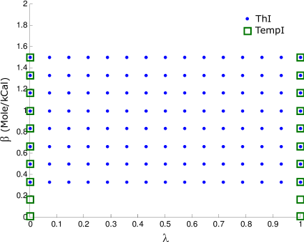
Figure 1: Illustration of the grid of values over which the Monte-Carlo simulations are performed in the two procedures: ThI with PT and TempI. The lowest values of $\beta$ correspond to some very high finite temperature.

2.3 Calculation of $\Delta F$ by Temperature Integration

We present now our method, which obtains the free energy difference $\triangle F_{A\rightarrow B}\left(\beta_{1}\right)$, using only simulations that are done in the process of parallel tempering, performed for the two systems $A$ and $B$,(eliminating the need for simulations at a set of $\lambda_{i}$ values). This method can be applied to any two systems that have the same degrees of freedom $\Omega$.

As $\beta\to 0$, the limiting value of the partition function of a system yields the phase space volume. In particular, if systems $A$ and $B$, which have the same coordinate space $\boldsymbol{\left\{\Omega\right\}}$, have the same $\beta\to 0$ limit, we have

$$Z_{B}\left(\beta\to 0\right)=Z_{A}\left(\beta\to 0\right)=\int d\boldsymbol{\Omega}\,.$$ (7)

In this case we can use the following identity to obtain, for a finite $\beta_{1}$, the difference of the free energies:

$$\ln Z\left(\beta_{1}\right)-\ln Z\left(\beta\to 0\right)=\int_{0}^{\beta_{1}}\frac{d\ln Z}{d\beta}d\beta=-\int_{0}^{\beta_{1}}\left\langle H\right\rangle d\beta\,$$ (8)

Using equations (7) and (8) we obtain

$$\triangle F_{A\rightarrow B}\left(\beta_{1}\right) = \frac{1}{\beta_{1}}\left[\ln Z_{A}\left(\beta_{1}\right)-\ln Z_{B}\left(\beta_{1}\right)\right]$$ (9)

$$= \frac{1}{\beta_{1}}\left[\intop_{0}^{\beta_{1}}\left\langle H_{B}\right\rangle d\beta-\intop_{0}^{\beta_{1}}\left\langle H_{A}\right\rangle d\beta\right]\,.$$

For each of the systems $A$ and $B$ we estimate the integrals on the right hand side by procedures of parallel tempering, sampling the system at a series of values $\beta_{1},\ldots,\beta_{n}$. We choose values such that the highest temperature sampled (corresponding to $\beta_{n}$) is much larger than the internal energy of the system at $\beta_{1}$, so $Z(\beta_{n})\simeq Z(\beta\to 0)$ is satisfied.

3 Comparing two systems with different partition functions at high Temperatures by introducing a cutoff

The condition of Equation (7) poses a problem for any two systems that have different partition functions values at high -$T$. In order to satisfy the condition stated above we had to set a cutoff over the interactions, $E_{\mathrm{cutoff}}$. We show that our results do not depend on the choice of $E_{\mathrm{cutoff}}$ and $\beta_{n}$, as long as $E_{\mathrm{cutoff}}$ is much larger than any typical interaction energy in the system at $\beta_{1}$, and $\beta_{n}^{-1}\gg E_{\mathrm{cutoff}}$.

Note that this use of cutoff is general and can be used for any energy term that differentiates between the systems at the high $T$ limit.

The proposed calculation of the free energy difference between the two systems at the temperature of interest $\beta_{1}$ is legitimate only if our choice of the cutoff energy has a negligible effect on the partition function value of each of the two systems at $\beta_{1}$. In addition, the highest temperature used, corresponding to $\beta_{n}$, must be such that the equality of the partition functions of the two systems is satisfied to a good accuracy.

We denote the Hamiltonian with the cutoff energy by $H^{\prime}$, and write the requirements stated above explicitly as follows:

$$lnZ_{B}\left(\beta_{1},H\right)\simeq lnZ_{B}\left(\beta_{1},H^{\prime}\right)$$ (10)

$$lnZ_{A}\left(\beta_{1},H\right)\simeq lnZ_{A}\left(\beta_{1},H^{\prime}\right)$$ (11)

$$lnZ_{B}\left(\beta_{n},H^{\prime}\right)\simeq lnZ_{A}\left(\beta_{n},H^{\prime}\right)$$ (12)

In order for the cutoff to have a negligible effect on the partition functions at the temperature of interest it has to be set to a value that satisfies

$$E_{\mathrm{cutoff}}\gg k_{\mathrm{B}}T_{1}.$$ (13)

As for $\beta_{n}$, if the cutoff energy satisfies

$$E_{\mathrm{cutoff}}\ll k_{\mathrm{B}}T_{n},$$ (14)

the systems will have almost equal probability to be in all the regions of their phase space, including ones which were restricted due to high energy values. Thus, the partition functions values of the two systems will be almost equal.

Hence if these requirements are satisfied one can write:

$$lnZ_{A}\left(\beta_{1},H\right)-lnZ_{B}\left(\beta_{1},H\right)\simeq$$

$$lnZ_{A}\left(\beta_{1},H^{\prime}\right)-lnZ_{B}\left(\beta_{1},H^{\prime}\right)\simeq$$

$$lnZ_{B}\left(\beta_{n},H^{\prime}\right)-lnZ_{B}\left(\beta_{1},H^{\prime}\right)$$

$$-\left[lnZ_{A}\left(\beta_{n},H^{\prime}\right)-lnZ_{A}\left(\beta_{1},H^{\prime}\right)\right]$$ (15)

Using the identity in Eq. (8), we can write:

$$\triangle F_{A\rightarrow{B}}\left(\beta_{1},H\right)=\frac{1}{\beta_{1}}\left[lnZ_{A}\left(\beta_{1},H\right)-lnZ_{B}\left(\beta_{1},H\right)\right]\simeq$$

$$\frac{1}{\beta_{1}}\left[\intop_{\beta_{n}}^{\beta_{1}}\left\langle H^{\prime}_{B}\right\rangle d\tilde{\beta}-\intop_{\beta_{n}}^{\beta_{1}}\left\langle H^{\prime}_{A}\right\rangle d\tilde{\beta}\right]$$ (16)

So the calculation of free energy will be negligibly affected by the use of a cutoff energy as long as we fulfill the relevant conditions.

This use of cutoff energy is relevant also to ThI and similar methods. Consider for example two systems, $H_{0}$ and $H_{1}$ that have different steric constraints (resulting in different $\beta\to 0$ limits), Then e.g. at $\lambda=0$ there may be micro-states with finite statistical weight $e^{-\beta H_{0}}$ and infinite energy in $H_{1}$, so the sampling of the internal energy $\langle H_{1}\rangle_{\lambda=0}$ is infeasible.

It can be seen that since the partition function of a system that has the Hamiltonian with the cutoff $H^{\prime}$ is almost equal to the one of a system with the Hamiltonian $H$ at $\beta_{1}$. Thus

$$\triangle F_{A\rightarrow{B}}\left(\beta_{1},H\right)\simeq\frac{1}{\beta_{1}}\left[lnZ_{A}\left(\beta_{1},H^{\prime}\right)-lnZ_{B}\left(\beta_{1},H^{\prime}\right)\right],$$ (17)

and ThI can be implemented for systems with $H^{\prime}$ and yield almost the same result.

In conclusion, with the use of cutoff energy in ThI, that enables us to sample the integrand in all cases, the free energy difference between any two systems that have the same degrees of freedom can be calculated.

4 Applying Temperature Integration to a toy model

In the following sections we present the results obtained by applying Temperature Integration with interaction cutoff to a “toy model”, of $N=8-25$ particles on a ring (one dimension, periodic boundary conditions) in an external potential, interacting via a hard core potential. For this model we evaluated the free energy difference between two systems, which differ in the size of their hard cores. We did this in two ways: First we performed ThI at a set of $\lambda$ values, where at each value the corresponding system was equilibrated using PT; second, we used Temperature Integration. We compared the results as well as the amount of (computational) work needed, for the two ways, to achieve similar accuracy. We estimated the gain in work (number of Monte Carlo steps needed) and the way it scales with the number of particles.

4.1 Definition of the model

Here we demonstrate the method for a toy model in one dimension with periodic boundary conditions: we place $N$ particles on the unit circle, with the position of a particle defined by an angle ($\theta=\left[0,2\pi\right]$). The particles are in an external potential, given by

$$V\left(\theta_{i}\right)=V_{0}\cdot cos\left(2\theta_{i}\right)$$ (18)

and have “hard core” interaction:

$$U\left(\theta_{i},\theta_{j}\right)=\left\{\begin{array}[]{cc}\infty&dist\left(\theta_{i},\theta_{j}\right)<W\\ 0&dist\left(\theta_{i},\theta_{j}\right)\geqslant W\end{array}\right.$$ (19)

Here $W$ is the size of a particle’s “core”, and $dist\left(\theta_{i},\theta_{j}\right)$ is the angle difference between the particles.

In order to apply TeI we introduced a cutoff of this potential, replacing $U\left(\theta_{i},\theta_{j}\right)$ by:

$$U\left(\theta_{i},\theta_{j}\right)=\left\{\begin{array}[]{cc}U_{\mathrm{cutoff}}&dist\left(\theta_{i},\theta_{j}\right)<W\\ 0&dist\left(\theta_{i},\theta_{j}\right)\geqslant W\end{array}\right.$$ (20)

where $U_{\mathrm{cutoff}}$ is the energetic cost of two particles having overlapping cores. The effect of the cutoff on the results of the calculation is negligible as shown below in 4.5.

We calculate the free energy difference between two systems $A$ and $B$, that have the same number of particles and different values of $W$. Specifically, we set the constants $V_{0},\,W$ in the systems $A,B$ to have the following values:

$$V_{0A}=V_{0B}=4,\qquad W_{A}=\frac{\pi}{4}\frac{1}{N},\qquad W_{B}=\frac{\pi}{8}\frac{1}{N}$$ (21)

We work at temperature $k_{\mathrm{B}}T_{1}=0.6157$ so that the barrier associated with the external potential is significantly higher than $k_{\rm B}T_{1}$, and set $U_{\mathrm{cutoff}}=70$, so that $U_{\mathrm{cutoff}}\gg k_{\mathrm{B}}T_{1}$ and hence condition (13) is satisfied.

4.2 Details of the Monte Carlo Simulation

In the initial configuration all the particles were placed in the interval $\left[0,\pi\right]$, at equal distances.

The local Monte Carlo move consists of randomly choosing one of the particles and changing its position $\theta$ to $\theta+\Delta\theta$, where $\Delta\theta\in\left[-\frac{\pi}{128},\frac{\pi}{128}\right]$ is selected with uniform probability.

All the Monte Carlo simulations are performed using Parallel Tempering; that is, after a certain number of local moves (500 in our case), we attempt to exchange configurations between systems at adjacent temperatures. We simulated systems with 8,10,12,14,17,20 and 25 particles and performed up to $\left(1,1.1,1.2,1.35,1.5,2\right)\cdot 10^{8}$ MC moves in total for each one respectively.

4.3 Using Thermodynamic Integration and PT

In order to compare the results obtained by TeI we used ThI in combination with PT. The set of temperatures at which we worked was selected as follows.

The highest temperature was chosen as $3V_{0}/k_{\mathrm{B}}$, to enable particles to cross easily the energy barrier ($2V_{0}$) of the external potential.

The temperatures for both systems $A$ and $B$ were first selected so that the acceptance rates for exchanging configurations at neighboring temperatures will be between $0.25$ and $0.35$. Then, the set of temperatures to be used was of that system in which the product of the acceptance rates was lower (i.e using the set of temperatures with higher density).

The integral in (16) was calculated by adding sampling points according to global adaptive Simpson’s quadrature (GASQ) [30, 31]. That is, for each value of $\lambda$, a simulation of a compound system was performed at the selected set of temperatures, and $\left\langle H_{B}(\mathbf{\boldsymbol{\Omega}})\right\rangle_{\lambda,\beta_{1}}-\left\langle H_{A}(\mathbf{\boldsymbol{\Omega}})\right\rangle_{\lambda,\beta_{1}}$ was calculated.

At each division of an interval, we sampled the internal energy at another 4 $\lambda$ values (according to GASQ [30, 31]), calculated the integral with the current set of intervals and displayed the result as a function of the total number of MC steps performed.

4.4 Using Temperature Integration

For each system, we evaluated numerically the integral:

$$k_{\mathrm{B}}T_{1}\intop_{\beta_{n}}^{\beta_{1}}\left\langle H\right\rangle d\beta$$ (22)

We chose $k_{\mathrm{B}}T_{n}$ to be given by $k_{\mathrm{B}}T_{n}=400*U_{0}*N*(N-1)/2$ in order to satisfy condition (14).

This was done iteratively. In each iteration we performed parallel tempering on a different set of temperatures and calculated the internal energies. Then, we added the results to those of the former iteration and calculated the integral (22) numerically according to the current set of sampling points ($\beta$-values and the corresponding internal energies).

After each calculation of the integral, we registered the result as well as the number of Monte Carlo steps performed in total until a stop criterion was reached (see Appendix).

The method by which we chose the sets of $\beta$-values was based on the global adaptive Simpson’s quadrature and was suited to maintain optimal acceptance rates between the systems (as explained in the Appendix).

4.5 Absolute Values of free energy and Verification of the method

The highest temperature $T_{n}$ was chosen to be much higher than the total interaction energy, so the partition function becomes the phase space volume, $\Omega$. Hence, when the phase space volume of a system is known at $T_{n}$, we can calculate the absolute (not relative) free energy of the system:

$$F=-k_{\mathrm{B}}T_{1}\left[\ln\frac{\Omega}{l^{3N}}+\int_{\beta_{n}}^{\beta_{1}}\left\langle H\right\rangle d\beta\right]\;,$$ (23)

where the integral in equation (23) can be estimated using the methods described in Section 2.3.

In many systems (including our toy model) when we neglect all interactions (including steric) the phase space volume is known and the values of free energy can be calculated according to (23), enabling the comparison of free energies of systems with different degrees of freedom.

To assess the accuracy of TempI (also in the context of absolute free energy values) for our toy model, we compared its result (for $N=3$ particles) with “exact enumeration” numerical evaluation of the free energy, obtained by performing with high precision the integral

$$F=-k_{\mathrm{B}}T_{1}\ln\left(\frac{\int e^{-\beta_{1}H}d\mathbf{\Omega}}{l^{3N}}\right)$$ (24)

In this integration, the microstates in which the steric limitations were violated weren’t taken into account, enabling us a liable comparison of the results according to (23).

4.6 Results

ThI (with PT) and TempI converged to the same asymptotic value of the $\Delta F_{A\to B}$ after a large enough number MC steps. The number of MC steps required for each method to approach the asymptotic value is, however, very different. In Fig. 2, we present the relation between the values of $\Delta F_{A\to B}$, calculated by the two methods, and its asymptotic value, as a function of the total number of the MC steps used in the calculation, for systems with 8, 17 and 25 particles. Evidently, in the TempI procedure the convergence of $\Delta F_{A\to B}$ to the asymptotic value was significantly faster than in ThI.

Figure 2: The result for $\Delta F$, normalized by the “asymptotic” value, as a function of the number MC steps using ThI and TempI, for systems with 8,17,25 particles.

Another measure of the relative efficiencies of the two methods is the number of MC steps needed to achieve a desired level of accuracy. In Fig. 3 we present the number of MC steps needed to approach the asymptotic value to within $1\%$, by both methods, as a function of the number of particles.

Figure 3: MC steps needed for $1\%$ convergence in both methods as a function of the number of particles, $N$.

The ratio between the number of MC steps needed for convergence in ThI and in TempI increases steeply with particle number, as demonstrated in Fig. 3. We also computed the absolute free energies for $N=3$ particles, by both TempI and by exact enumeration. The numerical results obtained by TempI, using (23), were:

$$F_{A} =-k_{\mathrm{B}}T_{1}\left[ln\Omega\left(T_{n}\right)+\int_{\beta_{n}}^{\beta_{1}}\left\langle H\right\rangle d\beta\right]$$ (25)

$$=-k_{\mathrm{B}}T_{1}\left[5.51+12.72\right]=-11.23$$ (26)

$$F_{B} =-k_{\mathrm{B}}T_{1}\left[5.51+13.40\right]=-11.64\;,$$ (27)

where the phase space volume is $\Omega=\left(2\pi\right)^{3}$. Numerical integration over the whole phase space yielded the same values, confirming the validity of our method in general and in the context of absolute free energy values.

5 Discussion

We presented Temperature Integration, a method to calculate the free energy difference between two systems at some inverse temperature $\beta_{1}$. Temperature Integration is an efficient method since the temperatures used in the parallel tempering procedure are used as intermediates in the calculation of free energy. Moreover, the method for choosing the intermediates for the calculation of free energy in TempI is general (see Appendix for details). Hence, the method is robust, which is important for automation and high-throughput use.

In the calculation, we performed parallel tempering procedures for each of the two systems over sets of temperatures between $\beta_{1}$ and $\beta_{n}$, where $\beta_{n}^{-1}\gg E_{\mathrm{cutoff}}$ - the maximal interaction energy of the system. Then, we use the internal energy values obtained at each temperature to estimate numerically the two integrals in equation (9), and hence the free energy difference between the two systems.

Furthermore, absolute values of the free energy can be calculated for systems in which the phase space volume is known (when all interactions are neglected) as stated in section 4.5.

TempI can be used also for systems with a smooth energy landscape (where PT is not needed). TempI has the advantage of simplicity (saves programming time) since the simulations are performed only on the two original systems (i.e. using only the two ”pure” Hamiltonians).

While in other methods for calculating free energy difference between two systems the choice of appropriate intermediates remains a challenge [20], in TempI the internal energy $\left\langle H\right\rangle$ is a monotonic function of $\beta$ and as a result the intermediates can be easily chosen (see appendix for details) and the calculation is much easier to verify. Moreover, the monotonicity of the function may result in less intermediates and facilitate the calculation (the number of integration points scales as the free energy difference which is roughly linear with the number of particles $N$).

The method was applied to calculate free energy differences in a toy model of hard rods on a 1-dimensional ring.

There is a provisional patent pending that includes the contents of this paper. This work was partially supported by the Leir Charitable Foundation (ED, AF) the Einstein Center for Theoretical Physics (NC) and the National Science Foundation under CHE-0713981 (CHM). We want to acknowledge Amir Marcovitz for his assistance.

Appendix: Integration method in the Temperature Integration procedure

We introduce the method in which the sets of $\beta$-values are chosen in the process of sampling the function in the TempI procedure. These sets have to be chosen in a way that will minimize the total error calculated according to the Simpson’s method and will satisfy optimal acceptance rates in the PT procedures.

We chose a temperature $T_{\mathrm{PT}}$ – higher than the energy barriers in the system. In each PT procedure we kept constant the number of $\beta$-values sampled within the range $\left[T_{1},T_{\mathrm{PT}}\right]$, used in the PT procedure, and added them to a set of $\beta$-values in the range $\left[T_{\mathrm{PT}},T_{n}\right]$.

In this method we first sample over the set of $\beta$-values chosen to satisfy optimal acceptance rates in the system, including the points $\left(\beta_{n}+\beta_{\mathrm{PT}}\right)/2$ and $\beta_{n}$, as defined here and in Sec. 4.4.

Second, we sample over a set of $\beta$-values that bisect the intervals of the former set. In the subsequent bisecting we take into account the facts that in the range $\left[T_{1},T_{\mathrm{PT}}\right]$ the requirements for PT go together with the ones needed for optimal sampling of the integral, and that in the range $\left[T_{\mathrm{PT}},T_{n}\right]$ the two requirements don’t necessarily correlate but the temperatures can be sampled independently of the value of the other temperatures in the set.

The 5 sampling points in the range $\left[T_{\mathrm{PT}},T_{n}\right]$ we now have form a subinterval according to ASQ. We further sample this subinterval according to GASQ until the maximal error in the range (defined by $\Delta x_{i}\Delta y_{i}$) is smaller than the maximal error in the range $\left[T_{1},T_{\mathrm{PT}}\right]$. The group of subintervals in this range will form a vector which will be called $v_{\mathrm{high\,temps}}$.

We now further bisect the sampling points in the range $\left[T_{1},T_{\mathrm{PT}}\right]$ in 2 PT procedures, with the subinterval with the maximal error in $v_{\mathrm{high\,temps}}$ (according to GASQ). We repeat this step, necessitating this time 4 PT procedures and the sampling of the 2 subintervals with maximal error in $v_{\mathrm{high\,temps}}$.

Then, we generate 2 arrays of vectors of subintervals in the first range. The first consists of the odd subintervals and the second of the even subintervals, each vector consisting of the subintervals that will be derived from the original subinterval. We perform a loop in which in each iteration, we choose one of the 2 arrays. Then we select in each vector in the array the subinterval with the maximal error and we add to the chosen set the subinterval with the maximal error in $v_{\mathrm{high\,temps}}$. We bisect the chosen set of subintervals and since each bisecting includes 4 sampling points, we perform 4 PT procedures in order to do so. Then the bisected subintervals are placed instead of the subinterval from which they were derived, and the integral is calculated. Thus, we proceed until a certain total error or to a maximal number of iterations is reached. In each calculation of the integral, the number of MC steps performed is registered.

References

- [1] Christophe Chipot and Andrew Pohorille. Free energy calculations: theory and applications in chemistry and biology, volume 86. Springer, 2007.
- [2] Daniel M. Zuckerman. Equilibrium Sampling in Biomolecular Simulations. Annual Review of Biophysics, 40(1):41–62, 2011.
- [3] D. Frenkel and B. Smit. Understanding molecular simulation: from algorithms to applications. Academic Press, Inc. Orlando, FL, USA, 1996.
- [4] M.R. Shirts, D.L. Mobley, and J.D. Chodera. Alchemical free energy calculations: Ready for prime time? Annual Reports in Computational Chemistry, 3:41–59, 2007.
- [5] Kurt Binder and Dieter W Heermann. Monte Carlo simulation in statistical physics: an introduction. Springer, 2010.
- [6] C.H. Bennett. Efficient estimation of free energy differences from monte carlo data. Journal of Computational Physics, 22(2):245–268, 1976.
- [7] S. Kumar, J.M. Rosenberg, D. Bouzida, R.H. Swendsen, and P.A. Kollman. The weighted histogram analysis method for free-energy calculations on biomolecules. i. the method. Journal of Computational Chemistry, 13(8):1011–1021, 1992.
- [8] R.W. Zwanzig. High-temperature equation of state by a perturbation method. i. nonpolar gases. The Journal of Chemical Physics, 22:1420, 1954.
- [9] J.G. Kirkwood. Statistical mechanics of fluid mixtures. The Journal of Chemical Physics, 3:300, 1935.
- [10] TP Straatsma and JA McCammon. Multiconfiguration thermodynamic integration. The Journal of chemical physics, 95:1175, 1991.
- [11] C. Jarzynski. Nonequilibrium equality for free energy differences. Physical Review Letters, 78(14):2690, 1997.
- [12] DA Hendrix and C. Jarzynski. A fast growth method of computing free energy differences. The Journal of Chemical Physics, 114:5974, 2001.
- [13] G.E. Crooks. Path ensembles averages in systems driven far-from-equilibrium. Arxiv preprint cond-mat/9908420, 1999.
- [14] Peter Kollman. Free energy calculations: applications to chemical and biochemical phenomena. Chemical Reviews, 93(7):2395–2417, 1993.
- [15] C.J. Woods, M. Malaisree, S. Hannongbua, and A.J. Mulholland. A water-swap reaction coordinate for the calculation of absolute protein-ligand binding free energies. Journal of Chemical Physics, 134(5):4114, 2011.
- [16] Y. Deng and B. Roux. Computations of standard binding free energies with molecular dynamics simulations. The Journal of Physical Chemistry B, 113(8):2234–2246, 2009.
- [17] TP Straatsma and HJC Berendsen. Free energy of ionic hydration: Analysis of a thermodynamic integration technique to evaluate free energy differences by molecular dynamics simulations. The Journal of chemical physics, 89:5876, 1988.
- [18] I.V. Khavrutskii and A. Wallqvist. Computing relative free energies of solvation using single reference thermodynamic integration augmented with hamiltonian replica exchange. Journal of Chemical Theory and Computation, 2010.
- [19] X.Y. Meng, H.X. Zhang, M. Mezei, and M. Cui. Molecular docking: A powerful approach for structure-based drug discovery. Current Computer-Aided Drug Design, 7(2):146–157, 2011.
- [20] J.D. Chodera, D.L. Mobley, M.R. Shirts, R.W. Dixon, K. Branson, and V.S. Pande. Alchemical free energy methods for drug discovery: progress and challenges. Current opinion in structural biology, 2011.
- [21] E. Darve and A. Pohorille. Calculating free energies using average force. The Journal of Chemical Physics, 115:9169, 2001.
- [22] C.Y. Lin, C.K. Hu, and U.H.E. Hansmann. Parallel tempering simulations of hp-36. Proteins: Structure, Function, and Bioinformatics, 52(3):436–445, 2003.
- [23] A.M. Ferrenberg and R.H. Swendsen. New monte carlo technique for studying phase transitions. Physical review letters, 61(23):2635, 1988.
- [24] H. Fukunishi, O. Watanabe, and S. Takada. On the hamiltonian replica exchange method for efficient sampling of biomolecular systems: Application to protein structure prediction. The Journal of chemical physics, 116:9058, 2002.
- [25] C.J. Woods, W. Jonathan, and M.A. King. The development of replica-exchange-based free-energy methods. The Journal of Physical Chemistry B, 107(49):13703–13710, 2003.
- [26] T. Rodinger and R. Pomès. Enhancing the accuracy, the efficiency and the scope of free energy simulations. Current opinion in structural biology, 15(2):164–170, 2005.
- [27] Y. Sugita, A. Kitao, and Y. Okamoto. Multidimensional replica-exchange method for free-energy calculations. The Journal of Chemical Physics, 113:6042, 2000.
- [28] U.H.E. Hansmann. Parallel tempering algorithm for conformational studies of biological molecules. Chemical Physics Letters, 281(1-3):140–150, 1997.
- [29] D.J. Earl and M.W. Deem. Parallel tempering: Theory, applications, and new perspectives. Physical Chemistry Chemical Physics, 7(23):3910–3916, 2005.
- [30] J.N. Lyness. Notes on the adaptive simpson quadrature routine. Journal of the ACM (JACM), 16(3):483–495, 1969.
- [31] M.A. Malcolm and R.B. Simpson. Local versus global strategies for adaptive quadrature. ACM Transactions on Mathematical Software (TOMS), 1(2):129–146, 1975.